Finite-Size Scaling Critical Behavior of Randomly Pinned Spin-Density Waves

Abstract

We have performed Monte Carlo studies of the 3D $XY$ model with random uniaxial anisotropy, which is a model for randomly pinned spin-density waves. We study $L\times L\times L$ simple cubic lattices, using $L$ values in the range 16 to 64, and with random anisotropy strengths of $D/2J$ = 1, 2, 3, 6 and $\infty$. There is a well-defined finite temperature critical point, $T_{c}$, for each these values of $D/2J$. We present results for the angle-averaged magnetic structure factor, $S(k)$ at $T_{c}$ for $L=64$. We also use finite-size scaling analysis to study scaling functions for the critical behavior of the specific heat, the magnetization and the longitudinal magnetic susceptibility. Good data collapse of the scaling functions over a wide range of $T$ is seen for $D/2J$ = 6 and $\infty$. For our finite values of $D/2J$ the scaled magnetization function increases with $L$ below $T_{c}$, and appears to approach an $L$-independent limit for large $L$. This suggests that the system is ferromagnetic below $T_{c}$.

I Introduction

The Harris-Plischke-Zuckermann modelHPZ73 has long been used to study the effects of random uniaxial anisotropy on ferromagnetism. The Hamiltonian of this random anisotropy model (RAM) is

$$H_{RAM}~{}=~{}-J\sum_{\langle ij\rangle}\vec{\bf S}_{i}\cdot\vec{\bf S}_{j}~{}-~{}D\sum_{i}(\hat{\bf n}_{i}\cdot\vec{\bf S}_{i})^{2}\,,$$ (1)

where each $\vec{\bf S}_{i}$, the dynamical on site $i$, is usually taken to be a classical three-component spin of unit length. Each $\hat{\bf n}_{i}$ is a time-independent unit vector. The $\hat{\bf n}$ on different sites are assumed to be uncorrelated random variables. $\sum_{\langle ij\rangle}$ is a sum over nearest neighbors on some lattice. In this work we will use a simple cubic lattice with periodic boundary conditions, and we will study the case of two-component ($n=2$) spins.

As was discussed in some detail in an earlier paper,Fis95 if one chooses the $\vec{\bf S}_{i}$ and the $\hat{\bf n}_{i}$ to be two-component vectors, then the Hamiltonian can be mapped onto a model of a spin-density wave (SDW) in an anisotropic material with an easy axis. For $XY$ spins, i.e. $n=2$, the Hamiltonian of the model may be rewritten as

$$H~{}=~{}-J\sum_{\langle ij\rangle}\cos(\phi_{i}-\phi_{j})~{}-~{}{D\over 2}\sum_{i}[\cos(2(\phi_{i}-\theta_{i}))~{}-~{}1]\,.$$ (2)

Each $\phi_{i}$ is a dynamical variable which takes on values between 0 and $2\pi$. The $\langle ij\rangle$ indicates here a sum over nearest neighbors on a simple cubic lattice of size $L\times L\times L$. We choose each $\theta_{i}$ to be an independent identically distributed quenched random variable, with the probability distribution

$$P(\theta_{i})~{}=~{}1/2\pi\,$$ (3)

for $\theta_{i}$ between 0 and $2\pi$. A constant term has also been added to the anisotropy, to make the Hamiltonian well-behaved in the limit $D/J\to\infty$.

In this work we will study Eqn. 2 on the simple cubic lattice over a range of $D/J$, using Monte Carlo simulations. The large increase in available computing resources over the last fifteen years makes possible significant improvements over the earlier results.Fis95 By studying a range of $L$, we will be able to learn about the stability of long-range order against random pinning which respects the Kramers degeneracy, such as alloy disorder, and the critical behavior of a SDW in an easy-axis material with this type of pinning.

II Random pinning effects

In the limit $D/J\to\infty$, often called the Ising limit, both analyticalDV80 ; HCB87 ; FH90 and numericalJK80 ; Fis95 ; TPV06 ; LLMPV07 calculations become substantially simplified. This is due to the fact that in this Ising limit the random anisotropy term in the Hamiltonian becomes a projection operator, and each spin has only two allowed states. It has been argued that for large $D/J$ the behavior is close to the $D/J=\infty$ limit as long as $T\ll D$.HCB87 It has also been found, however, that for $n=2$ at low temperatures and moderately large values of $D/J$ the magnetization per spin on $L\times L\times L$ simple cubic lattices, $|\vec{M}(L)|$, decreasesFis95 as the temperature, $T$, is lowered. This effect was not seen for $D/J=\infty$.

A similar effect is seen in the case of the random bond Ising model (RBIM), where the Nishimori gauge symmetry causes the magnetization to have a maximum at a finite $T$ on the Nishimori line.Nis81 ; HTPV07 The RBIM is the natural extensionCL77 ; Fis90 of the RAM to the case of Ising spins, $n=1$. Thus it should be expected that the phase diagram of the $n=2$ RAM has a close relation to that of the RBIM. However, there are aspects of the phase diagrams which remain somewhat mysterious. For example, Chen and LubenskyCL77 found that the critical exponents which describe the stability of the ferromagnet-spin glass-paramagnet multicritical point for the random bond model in $6-\epsilon$ dimensions are well-behaved for $n=1$, but become complex for $n=2$ and $n=3$. One interpretation of this puzzling result is that the multicritical point itself becomes unstable in $6-\epsilon$ dimensions, so that it becomes a region of the phase diagram, rather than a single point. In this expanded multicritical region one might expect to find quasi-long-range order (QLRO). Although an explicit calculation has not been done, a similar result would not be surprising for the RAM. The existence of QLRO in the RAM was first suggested by Aharony and PytteAP80 in 1980. They laterAP83 pointed out that higher order terms might make the correlation length, $\xi$, finite below $T_{c}$. FeldmanFel01 has argued that QLRO should be common in disordered magnets and similar systems.

Thus there are a number of possibilities available for the topology of the phase diagram. In a Cayley-tree mean-field theory, where QLRO does not occur, it is knownHCB87 that in the limit $D/J\to\infty$ the phase diagram depends on the parameter $z/n$, where $z$ is the number of nearest neighbor spins. Thus it is to be expected that the phase diagram in three dimensions will also depend on the lattice type, $n$ and the range of the exchange interactions, as well as on $T/J$ and $D/J$. For the simple cubic lattice (which has $z=6$) it has been shownLLMPV07 that in the limit $D/J\to\infty$ the ground state is an Ising spin glass when $n\geq 3$. For small $D/J$, however, where one does not expect the qualitative behavior to depend on $z$, FeldmanFel01 predicts QLRO in $d=3$ for $n\leq 4$. In the $n=3$ case, this appears to be confirmed by Monte Carlo calculations.Fis98

The presence of a reentrant phase is difficult to demonstrate conclusively using the type of numerical calculations we have performed here. It was only relatively recently that reentrance was demonstrated convincingly in the $d=2$ RBIM.WHP03 ; HTPV08 There may also be a range of $D/J$ for which the three-dimensional $n=2$ model has a reentrant ferromagnetic phase. One motivation for believing this is that reentrance is frequently observed in laboratory experiments. Another is the work of Pelcovits, Pytte and RudnickPPR78 ; Pel79 who argue that ferromagnetism should be unstable in the RAM for low $T$ and small $D/J$. Since magnetization can increase with increasing $T$ at low $T$, (which was not known at the time of their work,) it is not correct to claim that the absence of ferromagnetism near $T=0$ precludes the existence of a ferromagnetic phase in the RAM at a somewhat higher $T$.

LarkinLar70 studied a model for a vortex lattice in a type-II superconductor. His model replaces the spin-exchange term of the Hamiltonian with a harmonic potential, so that each $\phi_{i}$ is no longer restricted to lie in a compact interval. He argued that for any non-zero value of a random field this model has no long-range order on a lattice whose dimension $d$ is less than or equal to four. This argument, using the harmonic potential instead of the spin-exchange, is only rigorously correct in the limit $n\to\infty$.

A more intuitive derivation of the result was given by Imry and Ma,IM75 who assumed that the increase in the energy of an $L^{d}$ lattice when the order parameter is twisted at a boundary scales as $L^{d-2}$, just as it does in the nonrandom ferromagnet. As argued by Imry and Ma,IM75 and later justified more carefully,AIM76 ; PS82 within an $\epsilon$-expansion one finds the phenomenon of “dimensional reduction”. Within this perturbation theory the critical exponents of any $d$-dimensional $O(n)$ random-field model (RFM) (for which the Kramers degeneracy is broken by the randomness) appear to be identical to those of an ordinary $O(n)$ model of dimension $d-2$. For the Ising ($n=1$) case, this dimensional reduction was shown rigorously to be incorrect.Imb84 ; BK87 Another interesting development was the calculation of Mezard and Young,MY92 who showed that random fields caused breaking of replica symmetry below $T_{c}$ for any finite value of $n$. Thus there is no good reason to expect that dimensional reduction should be correct near $T_{c}$ for any finite value of $n$.

Although there is certainly a family resemblance between the RFM and the RAM, the difference between breaking the Kramers degeneracy at the level of Hamiltonian and breaking it spontaneously has profound consequences. One such consequence is Theorem 4.4 of Aizenman and Wehr,AW90 which applies to the RFM, but not to the RAM. A naive but not entirely misleading analogy may be drawn between the relationship of the RFM to the RAM and the relationship between applying a uniform magnetic field to a ferromagnet or to an antiferromagnet. The field which couples linearly to the order parameter has a qualitatively stronger effect than the field which couples quadratically to the order parameter.

Translation invariance of $H_{RAM}$ is broken for any non-zero value of $D$, since the vectors $\hat{\bf n}_{i}$ are random. Within a high-temperature perturbation theory, performing a configuration average over the ensemble of random lattices appears to restore translation invariance above $T_{c}$. However, the radius of convergence of this perturbation theory cannot be greater for $D\neq 0$ than it is for $D=0$. For models described by Eqn. (1), the $T_{c}$ predicted by extrapolating the low orders of perturbation theory is always maximal at $D=0$. This implies that for $D\neq 0$ the high-temperature perturbation theory does not converge near $T_{c}$. The inadequacy of perturbation theory to describe $XY$ models in $d=3$, because of the effects of vortex lines, has been discussed by Halperin.Hal81 While it is not clear than Halperin’s argument is valid for the RFM, where the Kramers degeneracy is broken by the Hamiltonian, it should be valid for the RAM. Thus it seems quite implausible that for $d<4$ the twist energy for Eqn. (2) really scales as $L^{d-2}$ when $D\neq 0$, even though this is correct to all orders in the configuration-averaged perturbation theory.

The argument of PelcovitsPel79 for the $n=2$ RAM, which is a prototype for much subsequent work,Fish85 assumes that if one goes to small enough $D/J$ and low enough $T$ then the effects of vortex lines can be ignored. In essence, what is done is to replace the spin variables by a noncompact ”elastic manifold”. These authors then claim that this does not effect the behavior one is studying. However, this cannot be true when one considers behavior on scales larger than the Imry-Ma length.Cop91

The basic point is that Imry-Ma-type arguments for continuous O(n) spins (i.e. $n\geq 2$) are not self-consistent. One begins by assuming that the random field is weak so that the twist energy scales as $L^{d-2}$, as in the absence of the randomness. Then one shows that, if $d\leq 4$ and $T<T_{c}$, the effective coupling to the random field increases as $L$ increases. If the effective random coupling is strong, however, then assuming that the twist energy is uniformly distributed throughout the volume is not reasonable. The conclusion which should be drawn from this is that a deeper analysis is needed when $d\leq 4$.

In order to understand whether the problems with perturbation theory are actually due to vortex lines, and thus restricted to the $n=2$ case, or if similar problems can also be expected for $n>2$, it may be helpful to reconsider the analysis of Pelcovits, Pytte and Rudnick.PPR78 These authors show that within their perturbation theory the pure O(n) mean-field theory critical fixed point remains stable against random anisotropy for $d>4$. This contrasts to the random-field case, where mean-field theory is only stable for $d>6$. Then they argue that for $d\leq 4$ and $n\geq 2$ there is no stable critical fixed point for the RAM, because under rescaling transformations the random anisotropy coupling constant runs off to $\infty$. However, they did not (and within their formulation could not) examine the possibility that there could exist another ferromagnetic critical fixed point at a large value of $D/J$. The reason why such an object may exist is that there exist alternative formulations of mean-field theoryDV80 ; HCB87 for the RAM in the limit $D/J\to\infty$.

It is useful to consider the generalization of Eqn. (2) to $p$-fold random fields.Aha81 In the $d=2$ caseHKY81 ; CO82 it has been shown that there continues to be a Kosterlitz-Thouless phase as long as $p^{2}>8$, i.e. for $p^{2}>8$ a weak $p$-fold random field does not destroy the Kosterlitz-Thouless phase. It was claimed by AharonyAha81 that ferromagnetism should be unstable for any value of $p$ when $d=3$. However, a computer simulation studyFis92 for $p=3$ is not consistent with this claim, which is based on the weak randomness perturbation theory around the $D=0$ model. This $d=3$ computer simulation finds that there is a mass gap at $T=0$, an effect which cannot be reproduced within the perturbation theory. The interpretation of this is that for $p\geq 3$ the thickness of a domain wall remains finite in the limit $L\to\infty$, i.e. the domain wall becomes localized by random pinning.

Removing vortex lines from the pure $XY$ model by letting the vortex fugacity become large forces the system into a ferromagnetic state at any temperature.KSW86 ; Fis95b This result is true even in the presence of a strong $p=2$ random anisotropy,Fis00 but the $p=2$ case is more complicated than $p\geq 3$. For $p=2$, as we shall see, the domain walls probably have a fractal structure, rather than becoming completely localized.

III Numerical results

In this work, we will present results obtained from heat bath Monte Carlo calculations. The data were obtained from $L\times L\times L$ simple cubic lattices with $16\leq L\leq 64$ using periodic boundary conditions. The calculations were done for a 12-state clock model, i.e. a ${\bf Z}_{12}$ approximationFis97 to the $XY$ model of Eqn. (2). The computer program was an adaptation of the code used recently for the $XY$ model in a random field,Fis07 modified to replace the random field term with the random 2-fold anisotropy term of Eqn. (2). For any integer value of the quantity $D/2J$ one can use a lookup table for the Boltzmann factors, because all the energies in the problem are then expressible as sums of integers and integer multiples of $\sqrt{3}$. The values of $D/2J$ for which data were obtained are 1, 2, 3, 6, and $\infty$.

The discretization of the phase space of the model has significant effects at very low $T$, but the effects at the temperatures we study here are expected to be negligible compared to our statistical errors. The probability distributions for the local magnetization of equilibrium states which are calculated for the ${\bf Z}_{12}$ model are found to have very small contributions from the third and higher harmonics of $\cos(\phi)$ and $\sin(\phi)$. This is strong evidence that the 12-state clock model is an accurate approximation to the $XY$ model within our range of parameters. The ${\bf Z}_{12}$ model shows equivalent behavior for $D$ and $-D$, unlike the ${\bf Z}_{6}$ model used earlier.Fis95

The program uses two independent linear congruential pseudorandom number generators, one for choosing the values of the $\theta_{i}$, and a different one for the Monte Carlo spin flips, which are performed by a single-spin-flip heat-bath algorithm. The code was checked by setting $D=0$, and seeing that the known behavior of the pure ferromagnetic system was reproduced correctly.

Each sample was started off in a random spin state at a temperature significantly above the $T_{c}$ for the pure model, and cooled slowly. Thermal averages for $S(\vec{\bf k})$ were obtained at a set of temperatures spanning the critical region.

Figure 1: Angle-averaged structure factor for $64\times 64\times 64$ lattices with $D/2J=1$ at $T=2.203125$. The axes are scaled logarithmically.

Figure 2: Angle-averaged structure factor for $64\times 64\times 64$ lattices with $D/2J=2$ at $T=2.1875$. The axes are scaled logarithmically.

Figure 3: Angle-averaged structure factor for $64\times 64\times 64$ lattices with $D/2J=3$ at $T=2.171875$. The axes are scaled logarithmically.

Figure 4: Angle-averaged structure factor for $64\times 64\times 64$ lattices with $D/2J=6$ at $T=2.078125$. The axes are scaled logarithmically.

Figure 5: Angle-averaged structure factor for $64\times 64\times 64$ lattices with $D=\infty$ at $T=1.921875$. The axes are scaled logarithmically.

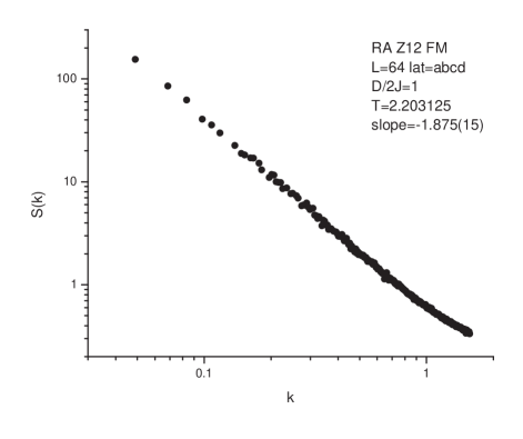
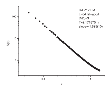
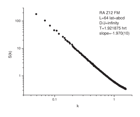
The magnetic structure factor, $S(\vec{\bf k})=\langle|\vec{\bf M}(\vec{\bf k})|^{2}\rangle$, for $n=2$ spins is

$$S(\vec{\bf k})~{}=~{}L^{-3}\sum_{i,j}\cos(\vec{\bf k}\cdot\vec{\bf r}_{ij})\langle\cos(\phi_{i}-\phi_{j})\rangle\,,$$ (4)

where $\vec{\bf r}_{ij}$ is the vector on the lattice which starts at site $i$ and ends at site $j$. Here the angle brackets denote a thermal average. For a RAM with $n>1$, unlike the RBIM, the longitudinal part of the magnetic susceptibility, $\chi_{l}$, which is given by

$$T\chi_{l}(\vec{\bf k})~{}=~{}1-M^{2}~{}+~{}L^{-3}\sum_{i\neq j}\cos(\vec{\bf k}\cdot\vec{\bf r}_{ij})(\langle\cos(\phi_{i}-\phi_{j})\rangle~{}-~{}Q_{ij})\,,$$ (5)

where $M^{2}~{}=~{}\langle|\vec{\bf M}|\rangle^{2}$, and $Q_{ij}~{}=~{}\langle\vec{\bf S}_{i}\rangle\cdot\langle\vec{\bf S}_{j}\rangle$. For O(2) spins

$$M^{2}~{}=~{}L^{-6}[\langle|\sum_{i}\cos(\phi_{i})|\rangle^{2}~{}+~{}\langle|\sum_{i}\sin(\phi_{i})|\rangle^{2}]\,,$$ (6)

and

$$Q_{ij}~{}=~{}\langle\cos(\phi_{i})\rangle\langle\cos(\phi_{j})\rangle~{}+~{}\langle\sin(\phi_{i})\rangle\langle\sin(\phi_{j})\rangle\,.$$ (7)

Thus $M^{2}$ is not the same as $S$, even above $T_{c}$. The scalar quantity $M^{2}$ is a well-behaved function of the lattice size $L$ for finite lattices, which approaches its large $L$ limit smoothly as $L$ increases, except possibly at a phase transition. The vector $\vec{\bf M}$, on the other hand, may not be a well-behaved function of $L$ for an $XY$ model in a two-fold random field. Knowing the local direction in which $\vec{\bf M}$ is pointing, averaged over some small part of the lattice, may not give us a strong constraint on what $\vec{\bf M}$ for the entire lattice will be.

The critical exponent $\eta$, is defined at $T=T_{c}$ by the small $\vec{k}$ behavior

$$S(\vec{\bf k})~{}\approx~{}c|\vec{\bf k}|^{-(2-\eta)}\,,$$ (8)

where $c$ is some constant. For each value of $D/J$, results for four different $L=64$ configurations of the random anisotropy $\theta_{i}$ were averaged. The same four samples of random $\theta_{i}$ were used for all values of $T$, and all values of $D/J$, in order to facilitate the comparison of results for different values of $T$ and $D$.

All of the data shown in these figures were obtained from Monte Carlo runs which used hot start initial conditions, starting at at temperature well above $T_{c}$. The value of $T$ was then lowered in steps. The initial part of the run at each $T$ was discarded to allow the system to equilibrate. For these $L=64$ runs with $D/2J$ = 1, at each $T$ a sequence of spin states obtained at intervals of 20,480 Monte Carlo steps per spin (MCS) was Fourier transformed and averaged. For the larger values of $D$, where the relaxation times are longer, this interval was chosen to be 102,400 MCS. The number of these selected spin states was chosen to be 16 for each of the finite values of $D/J$, and 32 for $D/J=\infty$. The Fourier transformed spin state data were then binned according to the values of $k$ = $|\vec{\bf k}|$, to give the angle-averaged $S(k)$. Finally, a configuration average over the four random samples was performed. Both equally weighted and logarithmically weighted averages were tried. No significant differences were found between these two types of weighting, and only the equally weighted averages will be displayed here.

The results for $D/2J$ = 1, 2, 3, 6, and $\infty$ are shown in Figs. 1, 2, 3, 4, and 5, respectively. The values of $T$ which are used in these figures are convenient binary fraction approximations to the values of $T_{c}$ at these values of $D/2J$. The best estimates of $T_{c}$ were determined later, by the analysis of the data over a range of $L$ and $T$. We see from these figures that $S(k)$ is only a weakly varying function of $D/J$, at least for $L=64$.

The values of $2-\eta$, as displayed on the figures, were found by least-squares fits to the data points for $0<k<\pi/8$, where the data are well-approximated by Eqn. 8. Note that $\eta$ appears to be a slowly varying monotonic function of $D/J$, and that the extrapolation of $\eta$ down toward $D$ = 0 appears to be significantly different from the value of $\eta$ found for the nonrandom $n=2$ ferromagnet.LGZJ80 ; LT89 It is also interesting to note that the value of $\eta$ found for $D=\infty$ appears to be identical to the value of $\eta$ for the nonrandom system, but the significance of this is unclear.

The fact that $\eta$ appears to vary with $D/J$ is an indication that the claim of ReedReed91 is too simplistic. He did not calculate a numerical value for $\eta$, but he argued that the finite-size scaling (FSS) behavior at $D/2J$ = 1 was indistinguishable from that of the nonrandom system.

One should not conclude from these data that $\eta$ is varying continuously with $D$, so that there is a line of critical points. Another explanation of the data is that for any $D$ we have a function $D_{eff}(D/J,L)$, which increases very slowly as $L$ increases, up to a value $D_{eff}=D^{*}$ Then we will only find $\eta_{eff}=\eta^{*}$ when $L$ becomes large enough so that $D_{eff}\approx D^{*}$. In the Cayley tree mean-field approximation,HCB87 whether $D^{*}$ is finite or infinite depends on the value of $z/n$.

Figure 6: (color online) Finite-size scaling near $T_{c}$ for $L\times L\times L$ lattices with $D/2J=1$. (a) Configuration-averaged magnetization vs. temperature. (b) $\chi_{l}$ vs. temperature. The $y$-axis is scaled logarithmically.

Figure 7: (color online) Finite-size scaling near $T_{c}$ for $L\times L\times L$ lattices with $D/2J=2$. (a) Configuration-averaged magnetization vs. temperature. (b) $\chi_{l}$ vs. temperature. The $y$-axis is scaled logarithmically.

Figure 8: (color online) Finite-size scaling near $T_{c}$ for $L\times L\times L$ lattices with $D/2J=3$. (a) Configuration-averaged magnetization vs. temperature. (b) $\chi_{l}$ vs. temperature. The $y$-axis is scaled logarithmically.

Figure 9: (color online) Finite-size scaling near $T_{c}$ for $L\times L\times L$ lattices with $D/2J=6$. (a) Configuration-averaged magnetization vs. temperature. (b) $\chi_{l}$ vs. temperature. The $y$-axis is scaled logarithmically.

Figure 10: (color online) Finite-size scaling near $T_{c}$ for $L\times L\times L$ lattices with $D/J=\infty$. (a) Configuration-averaged magnetization vs. temperature. (b) $\chi_{l}$ vs. temperature. The $y$-axis is scaled logarithmically.

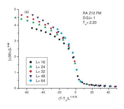
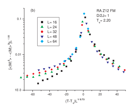
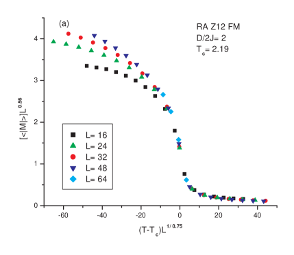
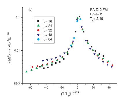
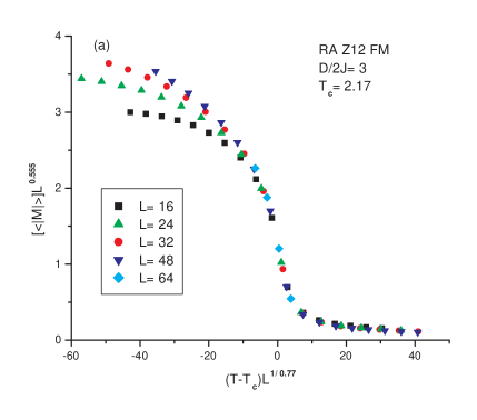
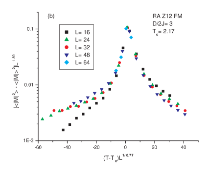
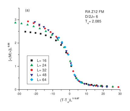
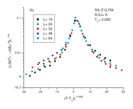
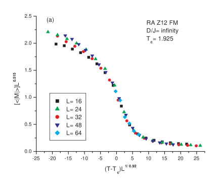
If we make the assumption that the usual critical exponent scaling laws for translation invariant models remain valid for the RAM, we can easily obtain values of the exponent combinations $\beta/\nu$ and $\gamma/\nu$ from our computed values of $2-\eta$. These combinations are exactly what we need for FSS of the magnetization $|\vec{\bf M}(L,T)|$ and the magnetic susceptibilityFB72 $\chi_{l}(L,T)$. Thus, by making standard FSS plots,NB99 we can test the validity of these scaling laws for the RAM.

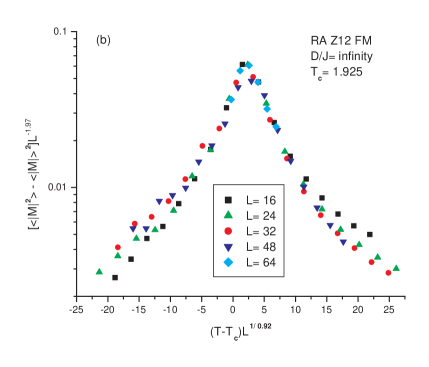
In Fig. 6(a) we show a FSS plot of the configuration average of $|\vec{\bf M}(L,T)|$ on $L\times L\times L$ lattices, for $L$ between 16 and 64. The number of sample configurations used for each $L<64$ was 8 for $D/2J$ = 1, 2, 3 and 6, and 16 for $D=\infty$. For $L$ = 64, the number of samples was 4 for all $D$. Fig. 6(b) shows a similar plot for $\chi_{l}$. Figs. 7, 8, 9 and 10 show the corresponding plots for $D/2J$ = 2, 3, 6 and $\infty$, respectively. Since the values of $\eta$ used here were taken from the fits to the small k behavior of $S(k)$, the only two adjustable fitting parameters used in these figures were the values of $\nu$ and $T_{c}$, which were required to be identical for parts (a) and (b) of each figure.

In these FSS plots, the temperature coordinate scales as $(T-T_{c})L^{1/\nu}$. The reader should note that the range of $T$ which we cover in these plots is about an order of magnitude larger than the range which one would typically use for a problem where one is already confident about the nature of the phase transition, and one is trying to obtain high precision estimates of $T_{c}$ and the critical exponents by concentrating on the range of $T$ where $\xi\approx L$. As a consequence of this, the spacings between the values of $T$ for which we have taken data are rather large. Thus we are unable to use histogram reweightingFLS95 to obtain essentially continuous values for the thermodynamic functions.

From the results given in these figures, we see that the estimates of $\nu$ increase monotonically and the estimates of $T_{c}$ decrease monotonically as $D/2J$ increases. We also see that the peak in $\chi_{l}$ is slightly above $T_{c}$ for finite $L$, which is typical for ferromagnetic critical behavior. The data collapse is good near this peak, which is the range of $T$ for which $\xi>L$. We do not give estimates of statistical errors for $\nu$, because we believe that the variation in $\nu$ in the range $D/2J$ = 1 to 6 is due to variation in the value of $D_{eff}$. We will discuss this further in the next section. The errors in the values of $T_{c}$ are estimated to be less than $\pm 0.01$.

Figure 11: (color online) Finite-size scaling of the difference between $c_{H}(T_{c})$= 3.00 and the configuration-averaged $c_{H}(L,T)$ vs. temperature near $T_{c}$ for $L\times L\times L$ lattices with $D/2J=1$.

Figure 12: (color online) Finite-size scaling of the difference between $c_{H}(T_{c})$= 2.65 and the configuration-averaged $c_{H}(L,T)$ vs. temperature near $T_{c}$ for $L\times L\times L$ lattices with $D/2J=2$.

Figure 13: (color online) Finite-size scaling of the difference between $c_{H}(T_{c})$= 2.40 and the configuration-averaged $c_{H}(L,T)$ vs. temperature near $T_{c}$ for $L\times L\times L$ lattices with $D/2J=3$.

Figure 14: (color online) Finite-size scaling of the difference between $c_{H}(T_{c})$= 1.94 and the configuration-averaged $c_{H}(L,T)$ vs. temperature near $T_{c}$ for $L\times L\times L$ lattices with $D/2J=6$.

Figure 15: (color online) Finite-size scaling of the difference between $c_{H}(T_{c})$= 0.81 and the configuration-averaged $c_{H}(L,T)$ vs. temperature near $T_{c}$ for $L\times L\times L$ lattices with $D=\infty$.

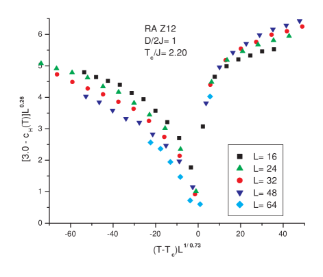
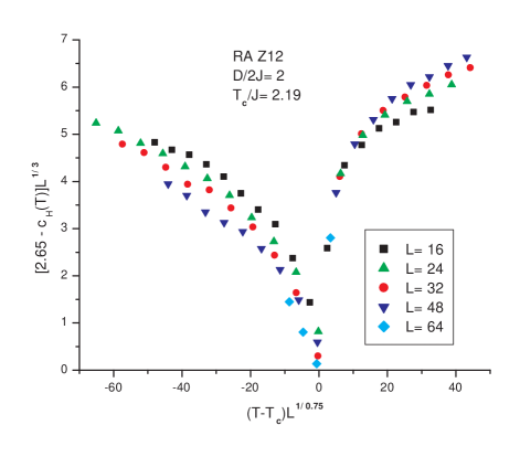
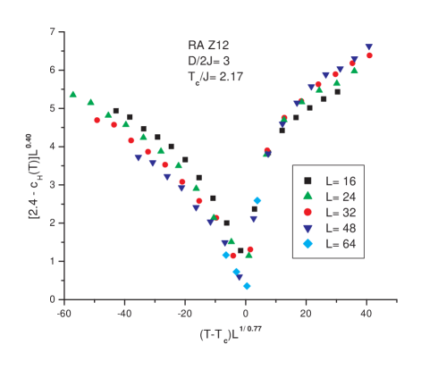
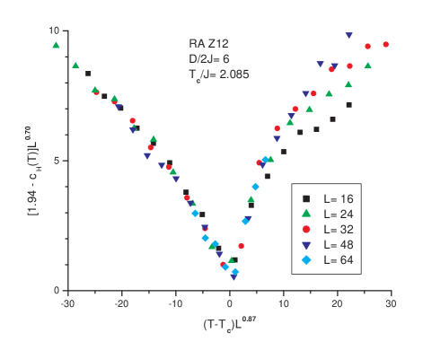
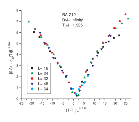
Fig. 11 shows the difference between an estimate of the specific heat at $T_{c}$ for an infinite system, $c_{H}(T_{c})$, and the calculated specific heat of a finite system at temperature $T$, $c_{H}(L,T)$ for $D/2J$ = 1. The only new adjustable fitting parameter here is $c_{H}(T_{c})$. Figs. 12, 13, 14 and 15 show the corresponding plots for $D/2J$ = 2, 3, 6 and $\infty$, respectively. The values of $c_{H}(T_{c})$ decrease monotonically as $D/2J$ increases. In all cases, the values of $c_{H}(T_{c})$ given in the figures are estimated to be accurate to about 1%. As we also saw for $|\vec{M}|$ and $\chi_{l}$, the FSS data collapse is not good below $T_{c}$ for $D/2J\leq 3$. The results for $D=\infty$ are in very good agreement with the earlier resultsFis95 obtained with the $Z_{6}$ approximation.

IV Discussion

According to Imry and MaIM75 and Pelcovits, Pytte and RudnickPPR78 , for small $D/J$ this model should appear ferromagnetic when $L$ is smaller than the ”Imry-Ma length”, which is determined by balancing the domain wall energy against the energy of random pinning. If this length exists, when $L$ is larger than the Imry-Ma length, the system will break up into domains, without long-range order. We have argued here, however, that in the presence of random pinning one should not believe that the domain wall energy scales as $L^{d-2}$. One can try to patch up this picture by assuming that the domain wall energy scales as $L^{d-\sigma_{dw}}$, with $3/2<\sigma_{dw}<2$. If this were the case, then it would still be possible for $d=3$ to find a length scale where the domain wall energy balanced the random pinning energy. Then it would continue to be true in $d=3$ that the system would break up into Imry-Ma-like domains when $L$ became very large.

What we see in our FSS plots for $D/2J\leq 3$, however, is that when $T<T_{c}$ the leading correction to finite-size scaling increases the magnetization as $L$ increases. Therefore this model appears to be stable against domain formation for $D/2J\leq 3$, at least for some range of $T$ below $T_{c}$. The natural interpretation of this result is that $\sigma_{dw}$ must be less than 3/2 in $d=3$ for the $n=2$ case.

Fig. 12, the FSS magnetization plot for $D/2J$ = 3, shows that as $L$ increases the data for $T<T_{c}$ seem to be converging to a scaling function which is independent of $L$. For the data in Fig. 15 for $D/2J$ = 6, the data appear to be in this $L$-independent limit. If we were able to do the Monte Carlo calculations at substantially larger values of $L$, we would expect to see the same type of convergence for $D/2J$ = 1 and 2.

If we had data at such large values of $L$, so that the magnetization scaling function had converged to an $L$-independent limit, then our estimates of the critical exponents would be expected to shift somewhat. Therefore, it is likely that $\eta^{*}$, the true value of $\eta$ in the range of $D/2J$ from 1 to 6, is actually independent of $D/J$.

The reader must also remember that the ferromagnetic phase is allowed to be reentrant. Therefore, we do not claim that the ferromagnetic behavior which we see below $T_{c}$ must be stable down to $T$ = 0 over the entire range of $D/J$. Also, we do not claim stable ferromagnetism for very large values of $D/J$. It must be stated, however, that this only applies to the simple cubic lattice with nearest neighbor interactions. We expect that it would be possible to stabilize a ferromagnetic phase at $D=\infty$ by adding further neighbor finite-range exchange interactions.

We point out that our earlier claimFis95 of infinite magnetic susceptibility without ferromagnetism when $D=\infty$ was based on results at $T=0$.Fis91 Since the magnetization of finite simple cubic lattices with $D=\infty$ seems to be a monotonically decreasing function of $T$,Fis95 however, we consider the existence of true ferromagnetism on this lattice to be unlikely at any $T$ for $D=\infty$.

The author sees no reason to believe that the exponent $\sigma_{dw}$ should be independent of $n$ for $d=3$. Thus, while we claim the existence of a ferromagnetic phase for $n=2$, we are not making any claim here about the behavior for $n=3$. We do expect that $\sigma_{dw}$ must converge to 2 in the limit $n\to\infty$, in agreement with the result of Larkin.Lar70 The reason for this is that for $n\to\infty$ the ”elastic membrane” approximation becomes valid.

Clearly, it would be desirable to obtain a direct estimate of $\sigma_{dw}$, by, for example, calculating the change in energy of a sample between periodic and antiperiodic boundary conditions along one direction. Since the energies involved are subextensive and the domain wall energy goes to zero at $T_{c}$, it is difficult to do such a calculation.

V Summary

In this work we have presented Monte Carlo results for the $d=3$ $XY$ random anisotropy model, Eqn. (2), for several values of the anisotropy strength $D/J$. By studying the finite-size scaling behavior of $L\times L\times L$ simple cubic lattices over the range $16\leq L\leq 64$, we find that, for values of $D/J$ which are not very large, there appears to be a finite-temperature critical point at which the model undergoes a transition into a ferromagnetic phase. For this lattice at very large $D/J$, the transition appears to be into a phase with QLRO, but no true magnetization.