Multiplicity fluctuations due to the temperature fluctuations in high-energy nuclear collisions

Abstract

We investigate the multiplicity fluctuations observed in high-energy nuclear collisions attributing them to intrinsic fluctuations of temperature of the hadronizing system formed in such processes. To account for these fluctuations we replace the usual Boltzmann-Gibbs (BG) statistics by the non-extensive Tsallis statistics characterized by the nonextensivity parameter $q$, with $|q-1|$ being a direct measure of fluctuations. In the limit of vanishing fluctuations, $q\rightarrow 1$ and Tsallis statistics converges to the usual BG. We evaluate the nonextensivity parameter $q$ and its dependence on the hadronizing system size from the experimentally observed collision centrality dependence of the mean multiplicity, $\langle N\rangle$, and its variance, $Var(N)$. We attribute the observed system size dependence of $q$ to the finiteness of the hadronizing source with $q=1$ corresponding to an infinite, thermalized source with a fixed temperature, and with $q>1$ (which is observed) corresponding to a finite source in which both the temperature and energy fluctuate.

I Introduction

With the large number of particles produced in heavy ion collisions at CERN SPS and BNL RHIC it is possible to study fluctuations in different physical observables on the event-by-event basis HH . These fluctuations are potentially a very important source of information on the thermodynamical properties of strongly interacting systems formed in such collisions, like, for example, its specific heat SS (connected with fluctuations observed in particle multiplicities NA49 ; WA98 , in transverse momenta NA49pT and in other global observables), its chemical potential or matter compressibility StM .

Fluctuations of multiplicity observed in heavy ion collisions exhibit spectacular and unexpected features as functions of the number of participants. Recent results on centrality dependence in $Pb+Pb$ collisions at $158$A GeV obtained by NA49 NA49 and WA98 WA98 experiments indicate that the scaled variance of the multiplicity distribution, $Var(N)/\langle N\rangle$, increases when proceeding from the central towards peripheral collisions, i.e., when the number of participants decreases. Such behavior is confirmed by a comprehensive survey of multiplicity fluctuations of charged hadrons provided by PHENIX experiment PHENIX .

During the last decade the statistical models of strong interactions were constantly used as an important tool to study fluctuation pattern observed in high energy nuclear collisions experiments, which are quantified by scaled variance mentioned above (see, for example, MIG1 ; MIG2 ; MIG3 and references therein). However, to minimize the effect of the possible participant number fluctuations, the analysis of particle number fluctuations has been restricted to the most central $A+A$ collisions only.

However, up to now, none of the models aimed to describe all essential features of multiparticle production processes (like multiplicities and distributions of particles in phase space and their composition) describe also the dependence of $Var(N)/\langle N\rangle$ on $N_{P}$, the number of nucleons from projectile nucleus participating in the collision - projectile participant, observed experimentally NA49 . They lead to multiplicity distributions of the (approximately) Poissonian form, independent of centrality, which highly underestimate the observed multiplicity fluctuations in noncentral collisions and thus are unable to reproduce, even qualitatively, the observed centrality dependence of the scaled variance. This remark applies not only to the Monte Carlo models like HIJING HIJING , HSD KLGB or UrQMD UrQMD , which are based on string excitation and decay, but also to any statistical model that does not assume correlations among secondary particles (cf. discussion in Sec. III.3). On the other hand, these results can be described by some specialized models addressing fluctuations directly, like the percolation model percolation , the model assuming inter-particle correlations caused by the combination of strong and electromagnetic interactions MW or the transparency, mixing and reflection model MixRefl . Fluctuations in these models reflect some dynamical features of the production process, (specific for the model considered).

In this paper we shall address the problem of multiplicity fluctuations without resorting to any specific dynamical picture but, instead, by attributing them to some nonstatistical, intrinsic fluctuations existing in a hadronizing system produced in high energy heavy ion collisions. To account for such fluctuations we shall use a special version of statistical model based on nonextensive Tsallis statistics Tsallis in which fluctuations of the temperature are known to be directly connected with the nonextensivity parameter $q$ WW ; BiroJ , namely $q=1+Var(1/T)/\langle 1/T\rangle^{2}$. In what follows they will be assumed to be the true (if not the only) origin of the fluctuations observed in the experimental data. The resulting distributions are then power-like, $\exp(-E/T)\Longrightarrow\exp_{q}(-E/T)=[1-(1-q)E/T]^{1/(1-q)}$ and in the limit of $q\rightarrow 1$ they go smoothly to the usual Boltzmann distributions (in what follows we shall address only the $q\geq 1$ case) FOOT3 . It is important for our further discussion that such non-exponential distributions of energy result in a non-Poissonian multiplicity distributions of the produced secondaries WWfluct .

However, to incorporate the new features of data reported by DataPi , we have to extend the notion of fluctuating temperature replacing it by some $q$-dependent effective temperature, $T_{eff}$, which accounts not only for the intrinsic fluctuations in the hadronizing source (as in WW ) but also for effects of the possible energy transfer taking place between the hadronizing source and its surroundings WW_epja . This will be done in Section II. Section III contains our results: the universal participant dependence (i.e., scaling in the variable $f=N_{P}/A$) presented in Section III.1, its explanation by the observation that in reality the hadronizing source is always of finite size presented in Section III.2 and the system size dependence of multiplicity and multiplicity fluctuations presented in Sections III.3. Section IV summarizes our work. Some details are presented in Appendices A and B.

II Effective temperature

In the proposed approach we replace the standard Boltzmann-Gibbs exponential distribution,

$$g(E)=C\exp(-E/T),$$ (1)

by the Tsallis distribution ($q$-exponential) defined as

$$h_{q}(E)=C_{q}\left[1-(1-q)\frac{E}{T_{eff}}\right]^{\frac{1}{1-q}},$$ (2)

where

$$q=1+\frac{Var(T)}{\langle T\rangle^{2}}.$$ (3)

Figure 1: (Color on line) Dependence of the effective temperature $T_{eff}$ (in GeV) on the parameter $q$ for the production in different reactions of negative pions $(a)$ and antiprotons $(b)$, all data points are from DataPi . The solid lines show linear fits to the obtained results: for upper panel $T_{eff}=0.22-1.25(q-1)$, for lower panel $T_{eff}=0.36-3.4(q-1)$.

and

$$T_{eff}=T_{0}+(q-1)\frac{1}{Dc_{p}\rho}\phi,$$ (4)

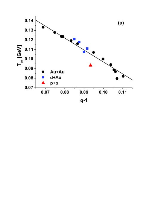
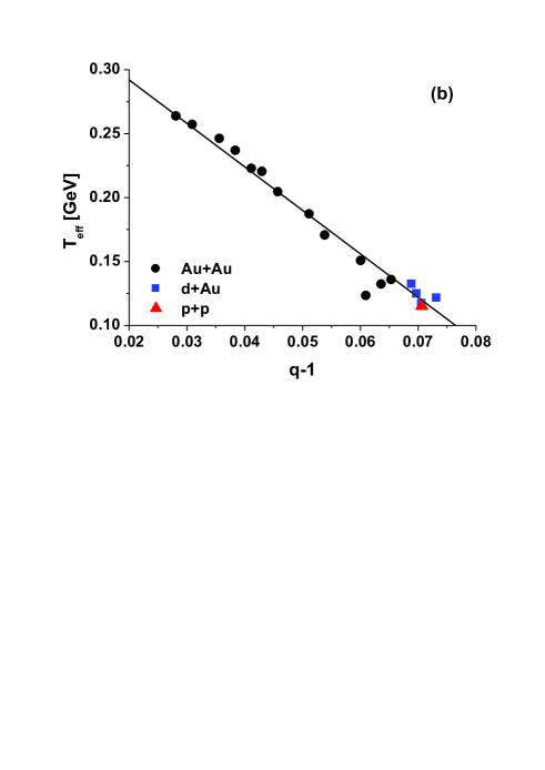
with $c_{p}$, $\rho$ and $D$ being, respectively, the specific heat under constant pressure, density and the strength of the temperature fluctuations (cf. Appendix A for details). Effective temperature $T_{eff}$ occurs when we experience both the fluctuations of the temperature $T$ (around the value $T_{0}$) and some energy transfer taking place between the source and the surroundings given by $\phi$ FOOT4 . Notice that in Eq. (4) energy transfer affects $T_{eff}$ only in the presence of fluctuations, i.e., for $q\neq 1$. The predicted $q$ dependence of $T_{eff}$ is indeed observed experimentally, cf. Fig. 1. Namely, in DataPi the transverse momentum spectra of pions and antiprotons produced in the interactions of p+p, d+Au and Au+Au at $\sqrt{s_{NN}}=200$ GeV at RHIC-BNL experiments DataPantiP were analyzed using a nonextensive approach in which the slope of $p_{T}$ distribution determines the effective temperature $T_{eff}$. Its shape gives the parameter of nonextensivity $q$ FOOT5 . They evaluated, among other things, the nonextensivity parameter $q$ and the effective temperature $T_{eff}$ for a different number of participants, $N_{P}$. From them we can deduce the dependence of $T_{eff}$ on the parameter $q$ which is shown in Fig. 1. Notice that in all cases we find that $\phi<0$ and that $T_{eff}$ seems to depend linearly on $(q-1)$. Negative values of $\phi$ mean that the energy is transferred from the interaction region to the surroundings (i.e., to the spectators of noninteracting nucleons) FOOT6 .

III Different facets of multiplicity fluctuations

III.1 The universal participant dependence

We start a discussion of multiplicity fluctuations by recollecting the result of WWfluct saying that if $N$ particles are distributed in energy according to the $N$-particle Tsallis distribution described by the nonextensive parameter $q$ then their multiplicity distribution has to be of the Negative-Binomial type with $k^{-1}=q-1$ (cf. Appendix B for details). It means therefore that we can expect that

$$\frac{\frac{Var(N)}{\langle N\rangle}-1}{\langle N\rangle}=q-1$$ (5)

(and, what is important, that $q-1$ determined this way does not depend on the acceptance of the detector FOOT-I ). On the other hand, if $U$ is the accessible energy and $gT_{eff}$ is the mean energy per particle detected in the acceptance region (with $g$ being a parameter and $T_{eff}$ effective temperature defined in Eq. (4)), than

$$\langle N\rangle=\frac{\langle U\rangle}{gT_{eff}}.$$ (6)

Using Eq. (4) one can shown that

$$\frac{\langle N\rangle-n_{0}N_{P}}{\langle N\rangle}=c(q-1),$$ (7)

where $n_{0}$ is the multiplicity in the single nucleon-nucleon collision measured in the region of acceptance, it is defined by the constraint that $\langle U\rangle=n_{0}gT_{0}N_{P}$, whereas $c=-\phi/\left(Dc_{p}\rho T_{0}\right)$ is a constant (notice that because in cases we are interested here $\phi<0$, cf. Fig. 1, $c$ is positive). Comparing now Eqs. (5) and (7) one can expect that

$$\frac{Var(N)}{\langle N\rangle}=1+c\left(\langle N\rangle-n_{0}N_{P}\right).$$ (8)

Notice that Eqs. (7) and (8) do not depend on parameter $g$ anymore; its role in present work is to fit, if necessary, $\langle N\rangle$ in Eq. (6) to experimental data only.

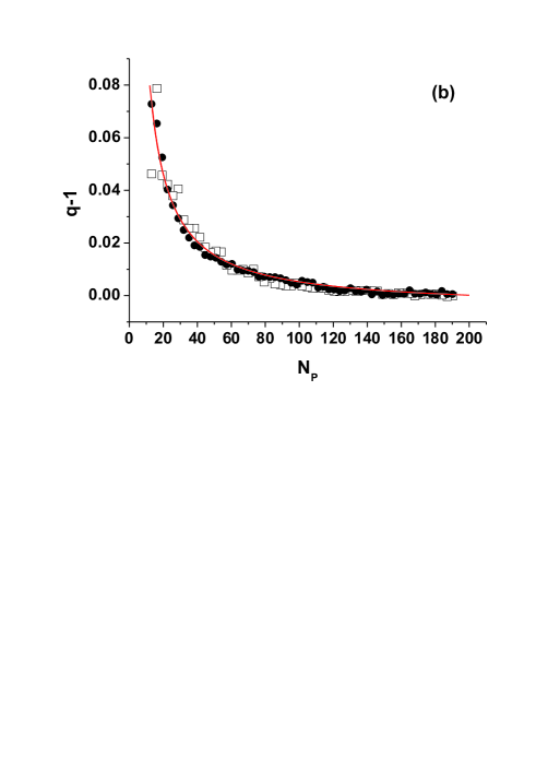
This means that using the notion of $T_{eff}$ one should observe that $Var(N)/\langle N\rangle$ and $\langle N\rangle$ are mutually connected. Fig. 2 shows that this is indeed the case. If $T_{eff}$ depends on $q$ (i.e., for $c\neq 0$) than the dependence $Var(N)/\langle N\rangle$ on the number of participants $N_{P}$ is connected to the dependence of $\langle N\rangle$ on $N_{P}$. Notice that if $\langle N\rangle$ is linear in $N_{P}$ then $Var(N)/\langle N\rangle$ is constant. In particular, for $\langle N\rangle=n_{0}N_{P}$ we have $Var(N)/\langle N\rangle=1$. Therefore the experimental fact that $Var(N)/\langle N\rangle$ decreases with increasing $N_{P}$ indicates nonlinear dependence of $\langle N\rangle$ on the number of participants $N_{P}$.

Figure 2: (Color on line) $(a)$ Comparison of $Var(N)/\langle N\rangle$ versus $N_{P}$ (squares) with $1+c(\langle N\rangle-n_{0}N_{P})$ versus $N_{P}$ (circles) for $n_{0}=0.642$ and $c=4.1$ FOOTA . Data are for negatively charged particles from $Pb+Pb$ collisions as collected by NA49 experiment NA49 . $(b)$ The same but translated to dependence of $q-1$ versus $N_{P}$. Squares were obtained from the $Var(N)/\langle N\rangle$ versus $N_{P}$ dependence whereas circles from the $\langle N\rangle$ versus $N_{P}$ dependence. The values of $n_{0}$ and $c$ are the same as before. The solid line shows the dependence (16) for the nuclear mass number $A=207$ and parameter $a=0.98$.

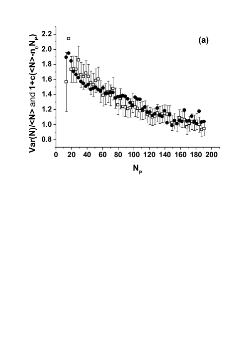
It should be stressed that data taken by the NA49 experiment NA49 show that $Var(N)/\langle N\rangle$ changes rather strongly with $N_{P}$. For peripheral collisions (i.e., for small $N_{P}$) one observes marked deviation of $Var(N)/\langle N\rangle$ from unity. At the same time deviation of $\langle N\rangle$ from linearity in $N_{P}$ is very weak. Our result based on the concept of effective temperature, $T_{eff}$, and showing that $Var(N)/\langle N\rangle$ and $\langle N\rangle$ are connected is therefore by no means trivial.

We close this Section by reminding that all previous attempts in this field were addressing only the behavior of $Var(N)/\langle N\rangle$ versus $N_{P}$, leaving aside the possible nonlinear dependence of $\langle N\rangle$ on $N_{P}$. Fig. 2 shows that introducing $T_{eff}$ results in a kind of scaling, namely the same value of $q-1$ describes dependencies of both variance and mean multiplicity on $N_{P}$, following Eq. (8), which - we repeat - has its origin in the $q$-dependence of $T_{eff}$ FOOT7 .

III.2 Finite hadronizing source size and temperature fluctuations

We shall now derive the $q-1$ dependence on $N_{P}$ seen in Fig. 2. Let us first observe that LL1 ; SS

$$q-1=\frac{Var(T)}{\langle T\rangle^{2}}=\frac{1}{C_{V}},$$ (9)

i.e., the parameter $q$ can be regarded as connected (via fluctuations of temperature) to the heat capacity under constant volume, $C_{V}$. For a system with finite size remaining in contact with a heat bath one has, following Lindhard’s approach Lin , that

$$Var(U)+C_{V}^{2}Var(T)=\langle T\rangle^{2}C_{V},$$ (10)

This is a kind of uncertainty relation (in the sense that it expresses the truth that in the case of conjugate variables one standard deviation in some measurement can only become small at the expense of the increase of some other standard deviation UnRel ). Relation (10) is supposed to be valid all the way from the canonical ensemble, where $Var(T)=0$ and $Var(U)=\langle T\rangle^{2}C_{V}$, to the microcanonical ensemble, for which $Var(T)=\langle T\rangle^{2}/C_{V}$ and $Var(U)=0$. Eq. (10) expresses both the complementarity between the temperature and energy, and between the canonical and microcanonical description of the system FOOT8 .

To obtain realistic (intermediate) distributions, start from a system at a fixed temperature $T$. The standard deviation of its energy is

$$Var(U)=\langle T\rangle^{2}\frac{\partial\langle U\rangle}{\partial T}=\langle T\rangle^{2}C_{V}.$$ (11)

Inverting the canonical distribution $g_{T}(U)$ one can obtain

$$g_{U}(T)=-T^{2}\frac{\partial}{\partial T}\int^{U}_{0}g_{T}(U^{\prime})dU^{\prime}$$ (12)

and interpret it as a probability distribution of the temperature in the system (cf., Eq. (36)). The standard deviation of this distribution then yields FOOT9

$$Var(T)=\frac{\langle T\rangle^{2}}{C_{V}}.$$ (13)

Because for a canonically distributed system the energy variance is $Var(U)=\langle T\rangle^{2}C_{V}$ and because for an isolated system $Var(U)=0$, for the intermediate case the variance (expressing energy fluctuations in the system) can be assumed to be equal to

$$Var(U)=\langle T\rangle^{2}C_{V}\xi,\quad\xi\in(0,1),$$ (14)

where the parameter $\xi$ depends on the size of the hadronizing source. Inserting this in Eq. (10) one gets that $q$ depends on $\xi$ in the following way:

$$q-1=\frac{Var(T)}{\langle T\rangle^{2}}=\frac{1-\xi}{C_{V}}.$$ (15)

Assuming now that the size of the thermal system produced in heavy ion collisions is proportional to the number of participating nucleons $N_{P}$, i.e., that $\xi\simeq f=N_{P}/A$, and taking into account that $C_{V}\cong aN_{P}$, we obtain that

$$q-1=\frac{1}{aN_{P}}(1-f).$$ (16)

This is the relation which nicely fits data, cf., Fig. 2.

To recapitulate: we know that if $U=$ const and $T=$ const then the multiplicity distribution $P(N)$ is Poissonian (cf. Appendix B.1) and we also know how fluctuations of $T$ change $P(N)$ from the Poissonian form to the NBD one (cf. Appendix B.2). We want now to see how big are fluctuations of $T$ in our hadronizing systems formed in a collision process. It turns out that for $N=$ const we have either Eq. (11) or Eq. (13) depending on whether $T=$ const or $U=$ const. We claim then that we can assume validity of Eq. (10) not only in the above limiting cases but also in the general case when both the energy $U$ and the temperature $T$ fluctuate at the same time, i.e., if fluctuations of the energy $U$ are given by Eq. (14) then fluctuations of the temperature $T$ are given by Eq. (15). Finally, knowing how big are fluctuations of $T$ we can deduce fluctuations of the multiplicity $N$. This will be performed in what follows.

III.3 System size dependence of mean multiplicity and multiplicity fluctuations

We shall now discuss, respectively, the system size dependence of the mean multiplicity and multiplicity fluctuations. In our approach the system size enters through $C_{V}$ and $\xi$. We shall keep $\xi=N_{P}/A$ and connect $C_{V}$ with the measured quantities considering two natural assumptions: either

$$C_{V}=aN_{P}$$ (17)

or

$$C_{V}=a^{\prime}\langle N\rangle.$$ (18)

When used together with Eqs.(7) and (15) the second possibility leads to a very simple scaling relation:

$$\langle N\rangle-\frac{N_{P}}{A}\langle N\rangle|_{N_{P}=A}=\frac{c}{a^{\prime}}\left(1-\frac{N_{P}}{A}\right)$$ (19)

whereas the first one results in a slightly more involved formula

$$\left(\langle N\rangle-\frac{N_{P}}{A}\langle N\rangle|_{N_{P}=A}\right)\frac{N_{P}}{\langle N\rangle}=\frac{c}{a}\left(1-\frac{N_{P}}{A}\right).$$ (20)

In both cases $\langle N\rangle|_{N_{P}=A}=n_{0}A$ is multiplicity extrapolated to $N_{P}=A$. As seen in Fig. 3, where comparison with experimental data NA49 is presented, one observes different dependencies for $Pb+Pb$ collision and lighter nuclei for which in semicentral collisions such an effect is practically not observed. In addition, for peripheral collisions ($N_{P}<0.15A$ ) one observes the deviation from the expected dependence (19). Notice that deviation from the linear fit for $Pb+Pb$ collisions concern only the $5$ most peripheral points and the observed discrepancy means that the measured experimentally mean multiplicity is less than $1$ particle higher than the expected value. The agreement with prediction given by Eq. (20) seems to be better, what means that the assumption $C_{V}=aN_{P}$ is more realistic.

Figure 3: (Color online) Mean multiplicities compared with predictions given by Eq.(20) $(a)$ and Eq.(19) $(b)$. We adopt $n_{0}=0.559$, $0.575$, $0.657$ and $0.642$ for, respectively, $p+p$, $C+C$, $Si+Si$ and $Pb+Pb$ collisions. Linear fit show the predictions of Eq. (19) with parameter $c/a^{\prime}=2.75$ and Eq. (20) with parameter $c/a=1.8$. Only statistical errors are indicated.

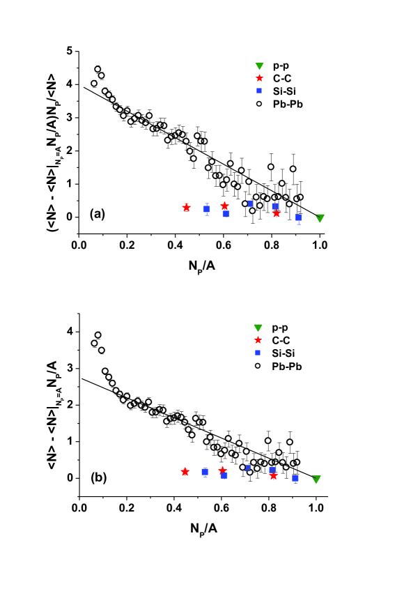
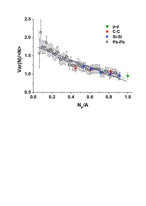
In what concerns multiplicity fluctuations, assumption (18) results (when combining Eqs. (16) and (5)) in the following simple scaling relation:

$$\frac{Var(N)}{\langle N\rangle}=1+\langle N\rangle(q-1)=1+\frac{1}{a^{\prime}}\left(1-\frac{N_{P}}{A}\right),$$ (21)

i.e., in the multiplicity fluctuations dependent on the fraction of nucleons participating in the collision $f=N_{P}/A$. Such scaling was found recently by the NA49 collaboration NA49 when comparing collisions of $C+C$, $Si+Si$ and $Pb+Pb$, cf. Fig. 4. If, instead, we use (17) then, taking into account dependence of $\langle N\rangle$ on $N_{P}$ given by Eq. (7), one obtains that, more exactly,

$$\frac{Var(N)}{\langle N\rangle}=1+\langle N\rangle(q-1)=1+\frac{n_{0}\left(1-\frac{N_{P}}{A}\right)}{a-\frac{c}{A}\left(\frac{A}{N_{P}}-1\right)}.$$ (22)

We observe thus a weak dependence on the mass number $A$ of colliding nuclei. For a small number of participants, $N_{P}<<A$, we observe an additional increase of relative variance, $Var(N)/\langle N\rangle$, in comparison with prediction (21). Notice that for $\phi>0$ one expects just the opposite trend, i.e., the non-monotonic behavior of $Var(N)/\langle N\rangle$ with increasing number of participants, $N_{P}$. The question about the sign of the heat source term $\phi$ seems to still be open due to the lack of data in the region of small number of participants.

For central collisions (i.e., for $f=N_{P}/A\simeq 1$) multiplicity distributions are sub-Poissonian and $[Var(N)/\langle N\rangle]|_{N_{P}=A}=\omega_{0}<1$. For example, within a statistical model with fixed volume $\omega_{0}$ varies in the range $0.5\div 1.0$ BGGZ . In particular (see MIG1 ; MIG3 and references therein): $(i)$ The global conservation laws imposed on each microscopic state of the statistical system lead to suppression of the particle number fluctuations. The final state scaled variance behavior in the canonical ensemble is characterized by $\omega_{0}\cong 0.8$ whereas in the microcanonical ensemble by $\omega_{0}\cong 0.3$. $(ii)$ In the primordial values of the scaled variance (i.e., calculated before decays of resonances) one can also observe the effect of quantum statistics. It turns out that proper inclusion of Bose statistics leads to the additional enhancement of particle number fluctuations of the order of $\omega_{0}\cong 1.05\div 1.06$, which is quite small at the chemical freeze-out. $(iii)$ The particle number fluctuations can be also enhanced by including explicite production and decay of resonances (either in the grand canonical ensemble of in canonical ensemble). They lead to $\omega_{0}\cong 1.1$. The actual value of parameter $\omega_{0}$ depends on the energy of collision and on the acceptance in which the multiplicity fluctuations are observed and varies in the range $0.8-1.0$ CAlt . For this reason in Fig. 4 we compare experimental data with the formula

$$\frac{Var(N)}{\langle N\rangle}=\omega_{0}+\frac{1}{a^{\prime}}\left(1-\frac{N_{P}}{A}\right).$$ (23)

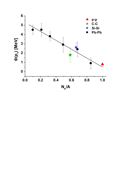
Finally, we note that the transverse-momentum fluctuations measured in nuclear collisions at $158$A GeV NA49pT and quantified by the measure $\Phi\left(p_{T}\right)$ FOOT10 show a similar centrality dependence, namely, as seen in Fig. 5,

$$\Phi\left(p_{T}\right)=\Phi_{N_{P}=A}+b\left(1-\frac{N_{P}}{A}\right).$$ (24)

This behavior of the transverse-momentum fluctuations as a function of collision centrality was related in superposition model to the centrality dependence of the multiplicity fluctuations MRW using the correlation of average transverse momentum and multiplicity observed in collisions NA49pT . To derive Eq. (24) notice that in general $\Phi$ is governed by the multiplicity fluctuations in the following way RWW :

$$\Phi\left(p_{T}\right)=\sqrt{Var\left(p_{T}\right)+2\langle p_{T}\rangle^{2}\frac{Var(N)}{\langle N\rangle}\left[1-\rho\sqrt{\frac{Var\left(p_{T}\right)}{\langle p_{T}\rangle^{2}}\frac{\langle N\rangle}{Var(N)}+1}\right]}-\sqrt{Var\left(p_{T}\right)},$$ (25)

where $\rho$ is the correlation coefficient between $N$ and $\sum^{N}_{i}p_{iT}$. As in MRW we can see that multiplicity fluctuations determine the behavior of $\Phi\left(p_{T}\right)$. In the first order approximation and taking into account multiplicity fluctuations given by Eq.(23) we can write the transverse momentum fluctuations measure as

$$\Phi\left(p_{T}\right) \simeq \sqrt{Var\left(p_{T}\right)}\left[\omega_{0}(1-\rho)\frac{\langle p_{T}\rangle^{2}}{Var\left(p_{T}\right)}-\frac{1}{2}\rho\right]+$$

$$+ \!\!\!\!\!\!\!\!\!(1-\rho)\sqrt{Var\left(p_{T}\right)}\frac{\langle p_{T}\rangle^{2}}{Var\left(p_{T}\right)}\frac{1}{a^{\prime}}\left(1-\frac{N_{P}}{A}\right),$$ (26)

which has the form of Eq. (24) in what concerns dependence on the variable $N_{P}/A$. The slope parameter $b$ corresponds to the correlation coefficient $\rho\sim 0.99$ (for the previously estimated value of $a^{\prime}$ and for the transverse momentum fluctuations $Var(p_{T})/\langle p_{T}\rangle^{2}\simeq 0.43$, as observed experimentally CERES ). Once again we observe scaling behavior in the variable $f=N_{P}/A$.

Figure 4: (Color online) The scaled variance of the multiplicity distribution of negatively charged particles produced in p+p, semicentral C+C, semicentral Si+Si, and Pb+Pb collisions as function of the fraction of nucleons participating in the collision, $N_{P}/A$. The experimental data NA49 are compared with prediction (23) with parameters $\omega_{0}=0.79$ and $a^{\prime}=1.0$ (solid line) and with prediction (22) with parameters $\omega_{0}=0.87$ and $a=0.83$ (dashed line, the other parameters are the same as in Fig. 2 with $n_{0}=0.642$ and $c=4.1$ for $A=207$).

Figure 5: (Color online) Transverse momentum fluctuations of negative particles defined by the measure $\Phi$ PHI as a function of number of the fraction of nucleons participating in the collision, $N_{P}/A$. The triangles correspond to $p+p$ collisions, asterisks to $C+C$, squares to $Si+Si$, and circles to $Pb+Pb$. The experimental data are taken from NA49pT and are compared with prediction of Eq.(24) for parameters $\Phi_{N_{P}=A}=0.48$ MeV and $b=4.8$ MeV.

IV Summary

We have investigated some features of the multiplicity fluctuations observed in recent high-energy nuclear collisions by attributing them to the intrinsic, nonstatistical, fluctuations of the temperature of the hadronizing system produced in such collisions. To this end we used the Tsallis statistics approach in which such fluctuations are accounted for by the nonextensivity parameter $q$ (more precisely by $q-1$). When fluctuations are vanishing $q\rightarrow 1$, Tsallis statistics becomes the usual Boltzmann-Gibbs (BG) one and the power-like Tsallis $q$-exponents become the usual exponential distributions. We were considering a generalized $q$-exponential ensemble describing system of $N_{P}$ participating nucleons (assumed to be proportional to the size of hadronizing system). It was found that in this case one can associate the nonextensivity parameter $q$ with the number of participants $N_{P}$ (cf. Eq.(16)). It was found that data require a generalization of the usual notion of fluctuating temperature by adding effects of the energy transfer between the hadronizing source and the surroundings composed with nucleons not participating directly in the reaction. This resulted in the introduction of a $q$-dependent effective temperature $T_{eff}$. We have also allowed for fluctuations of the full accessible energy $U$ (cf., Section III.1), without these fluctuations $Var(N)/\langle N\rangle$ would be simply constant, independent of $N_{P}/A$.

The simplest possible explanation of the observed effect was the $q-1$ dependence on the number of participants $N_{P}$ provided by the Eq.(16). We assumed that parameter connected with the size of the collision region, $\xi$, is approximately given by $\xi=N_{P}/A$. The modifications of this assumption are possible and lead to better agreement with experimental data. Among others, the presence of nonlinear terms in the $\xi$ variable in Eq.(15) would approve consistency with data (or, for example, assuming that $\xi=\zeta(N_{P}/A)$ with $\zeta(N_{P}/A)$ more complicated as used here where $\zeta(N_{P}/A)=N_{P}/A$). Nevertheless, we restricted our discussion to the simplest possible approximation to demonstrate the connection between temperature fluctuations and observables from relativistic ion collisions in a more transparent way.

Let us close with some remarks concerning limitations of our analysis. Firstly, let us first remind that multiplicity fluctuations considered in this study were observed for a fixed number of the projectile participants. Although, in the collisions of identical nuclei, the average numbers of the participants from the projectile equal approximately that from the target, the actual number of target participants fluctuate whereas the number of the projectile participants is kept fixed. However, one should notice that the multiplicity fluctuations were measured in the forward hemisphere ($1.1<y_{c.m.}<2.6$) in which the influence from the target participants is marginal. The models which produce, independently of centrality, approximately Poissonian multiplicity distributions highly underestimate the observed multiplicity fluctuations in noncentral collisions. They are unable to reproduce, even qualitatively, the centrality dependence of the scaled variance (cf., for example, NA49 and references therein). The highest scaled variance is obtained from the hadron-string dynamics KLGB and ultrarelativistic molecular dynamics UrQMD . However, both approaches (in their standard versions) show a flat scaled variance, $\omega\simeq 1.2$, and exhibit almost no dependence on $N_{p}$ MIG4 . Finally, note that in comparison with experimental data (which have finite acceptance, equal to $p=0.16$ in the case of NA49 data NA49 ) we have used multiplicity $N$ given by this acceptance. Also all parameters used for description of these data (like $n_{0}$, $a^{\prime}$, $\omega_{0}$, $\Phi_{N_{p}=A}$ and $b$) are acceptance dependent, However, as shown in FOOT-I , the nonextensivity parameter $q$ and its dependence on $N_{p}$ obtained from comparison with experimental data does nor depend on experimental acceptance.

Appendix A Temperature fluctuations

We shall collect here the main points concerning the idea of temperature fluctuations WW ; WW_epja .

Suppose that we have a nonhomogeneous thermodynamic system in different regions of which there is different temperature $T$, which fluctuates around some mean temperature $T_{0}$. As result of these fluctuations, the actual temperature $T$ equals

$$T=T_{0}-\xi(t)T,$$ (27)

where $\xi(t)$ describes the actual (not specified) stochastic process causing these fluctuations.

There must take place an exchange of energy (heat) between the regions mentioned above, in particular between any selected region and the rest of the system. This exchange eventually leads to equilibration of the temperature of the whole system. The corresponding process of heat conductance is described by the following equation LL :

$$c_{p}\rho\frac{\partial T}{\partial t}-\gamma(T^{\prime}-T)=\phi,$$ (28)

where $c_{p}$, $\rho$ and $\gamma$ are, respectively, the specific heat under constant pressure, the density and the coefficient of external conductance. The heat source term $\phi$ determines the amount of energy transfer per unit time and unit volume. Using Eqs. (27) and (28) one gets the following Langevine equation for the temperature $T$:

$$\frac{\partial T}{\partial t}+\left[\frac{1}{\tau}+\xi(t)\right]T=\frac{1}{\tau}\left[T_{0}+\frac{\tau}{c_{p}\rho}\phi\right]$$ (29)

with coefficient $\tau=c_{p}\rho/\gamma$. As stated before, $\xi(t)$ describes stochastic changes of temperature in time. Let us assume that these changes are such that their mean value is zero,

$$\langle\xi(t)\rangle=0,$$ (30)

whereas, for sufficiently fast changes, its correlator is equal to

$$\langle\xi(y)\xi(t+\Delta t)\rangle=2D\delta(\Delta t).$$ (31)

The constants $\tau$ and $D$ define, respectively, the characteristic mean time for the temperature changes and their variance:

$$\langle T(t)\rangle = T_{0}+T(t=0)\exp\left(-\frac{t}{\tau}\right),$$ (32)

$$\langle T^{2}(t=\infty)\rangle = \frac{1}{2}D\tau.$$ (33)

Thermodynamic equilibrium in such a situation means that for $t>>\tau$ the influence of the initial condition $T(t=0)$ vanishes and the mean squared $T$ has a value corresponding to the state of equilibrium.

Eq. (29) leads to the corresponding Fokker-Planck equation,

$$\frac{df(T)}{dt}=-\frac{\partial}{\partial T}K_{1}f(T)+\frac{1}{2}\frac{\partial^{2}}{\partial T^{2}}K_{2}f(T),$$ (34)

where the intensity coefficients are

$$K_{1}(T) = \frac{1}{\tau}\left(T_{0}+\frac{\tau}{c_{p}\rho}\phi\right)+\left(D-2\frac{1}{\tau}\right)T,$$

$$K_{2}(T) = 2DT^{2}.$$ (35)

Its solution is gamma distribution in $1/T=\beta$:

$$f(T)=\frac{\mu}{\Gamma(\alpha)}\left(\frac{\mu}{T}\right)^{\alpha-1}\exp\left(-\frac{\mu}{T}\right),$$ (36)

where

$$\alpha=\frac{1}{\tau D},\quad\mu=\frac{1}{\tau D}\left(T_{0}+\frac{\tau}{c_{p}\rho}\phi\right).$$ (37)

The mean value and the relative variance of $\beta$ are, respectively FOOT11 ,

$$\langle\beta\rangle=\left(T_{0}-\frac{\tau}{c_{p}\rho}\phi\right)^{-1},$$ (38)

$$\frac{\langle\beta^{2}\rangle-\langle\beta\rangle^{2}}{\langle\beta\rangle^{2}}=\frac{1}{\alpha}=\tau D.$$ (39)

Temperature fluctuations in the form presented here when applied to the exponential Boltzmann-Gibbs formula, Eq. (1), lead to $h_{q}(E)=\int_{0}^{\infty}\exp(-E/T)f(T)d(1/T)$, i.e., to a Tsallis distribution, Eq. (2), with the nonextensivity parameter $q$ equal to WW

$$q=1+\frac{1}{\alpha}=1+\tau D$$ (40)

and with the effective temperature

$$T_{eff}=T_{0}+\frac{\tau}{c_{p}\rho}\phi=T_{0}+(q-1)\frac{1}{Dc_{p}\rho}\phi.$$ (41)

In the case of no energy transfer, i.e., when $\phi=0$, one is left only with fluctuations and then $T_{eff}=T_{0}$, as in WW . Recently temperature fluctuations due to the volume fluctuations in statistical models were discussed as well and introduced in modelling of relativistic particle collision processes BGG .

Appendix B Multiplicity distributions in Boltzmann and Tsallis ensembles

We shall now recapitulate some basic ideas concerning multiplicity distributions which result from, respectively, Boltzmann and Tsallis ensembles WWfluct .

B.1 Poisson multiplicity distribution

This distribution arises in situations where, in some process, one has $N$ independently produced secondaries with energies $\{E_{1,\dots,N}\}$ distributed according to a Boltzmann distribution:

$$g(E_{i})=\frac{1}{\lambda}\exp\left(-\frac{E_{i}}{\lambda}\right);\quad{\rm where}\quad\lambda=\langle E\rangle.$$ (42)

The corresponding joint probability distribution is given by

$$g\left(\{E_{1,\dots,N}\}\right)=\frac{1}{\lambda^{N}}\exp\left(-\frac{1}{\lambda}\sum^{N}_{i=1}E_{i}\right).$$ (43)

For independent energies $\{E_{1,\dots,N}\}$ the sum $E=\sum^{N}_{i=1}E_{i}$ is distributed according to a gamma distribution,

$$g_{N}(E)=\frac{1}{\lambda(N-1)!}\left(\frac{E}{\lambda}\right)^{N-1}\exp\left(-\frac{E}{\lambda}\right),$$ (44)

the distribuant of which is

$$G_{N}(E)=1-\sum^{N-1}_{i=1}\frac{1}{(i-1)!}\left(\frac{E}{\lambda}\right)^{i-1}\exp\left(-\frac{E}{\lambda}\right).$$ (45)

Eq. (44) follows immediately either by using characteristic functions or by sequentially performing integration of the joint distribution (43) and noticing that

$$g_{N}(E)=g_{N-1}(E)\frac{E}{N-1}.$$ (46)

For energies such that

$$\sum^{N}_{i=0}E_{i}\leq E\leq\sum^{N+1}_{i=0}E_{i},$$ (47)

the corresponding multiplicity distribution has a Poissonian form (with $\langle N\rangle=\frac{E}{\lambda}$)

$$P(N)=G_{N+1}(E)-G_{N}(E)=\frac{\langle N\rangle^{N}}{N!}\exp(-\langle N\rangle).$$ (48)

Therefore, whenever $N$ variables $\{E_{1,\dots,N,N+1}\}$ follow an exponential distribution (42) and satisfy condition (47), then the corresponding multiplicity $N$ has a Poissonian distribution (48).

B.2 Negative Binomial multiplicity distribution

This distribution arises when in some process $N$ independent particles with energies $\{E_{1,\dots,N}\}$ are distributed according to a Tsallis distribution,

$$h\left(\{E_{1,\dots,N}\}\right)=C_{N}\left[1-(1-q)\frac{\sum^{N}_{i=1}E_{i}}{\lambda}\right]^{\frac{1}{1-q}+1-N}.$$ (49)

It means that there are some intrinsic (so far unspecified but summarily characterized by the parameter $q$) fluctuations present in the system under consideration. In this case we do not know the characteristic function for the Tsallis distribution. However, because we are dealing here only with variables $\{E_{1,\dots,N}\}$ occurring in the form of the sum, $E=\sum^{N}_{i=1}E_{i}$ , one can still sequentially perform integrations of the joint probability distribution (49) arriving at the formula corresponding to Eq. (44):

$$h_{N}(E) = h_{N-1}(E)\frac{E}{N-1}=\frac{E^{N-1}}{(N-1)!\lambda^{N}}\cdot$$ (50)

$$\cdot \!\!\!\!\!\!\!\!\!\!\prod^{N}_{i=1}[(i-2)q-(i-3)]\left[1-(1-q)\frac{E}{\lambda}\right]^{\frac{1}{1-q}+1-N}$$

with distribuant given by

$$H_{N}(E)=1-\sum^{N-1}_{j=1}\tilde{H}_{j}(E)$$ (51)

where

$$\tilde{H}_{j}(E) = \frac{E^{j-1}}{(j-1)!\lambda^{j}}\cdot$$ (52)

$$\cdot \!\!\!\!\!\!\!\!\!\!\prod^{j}_{i=1}[(i-2)q-(i-3)]\left[1-(1-q)\frac{E}{\lambda}\right]^{\frac{1}{1-q}+1-j}.$$

As before, for energies $E$ satisfying the condition given by Eq.(47), the corresponding multiplicity distribution is equal to the well known Negative Binomial distribution (NBD):

$$P(N) = H_{N+1}(E)-H_{N}(E)=$$

$$= \frac{(q-1)^{N}}{N!}\frac{q-1}{2-q}\frac{\Gamma\left(N+1+\frac{2-q}{q-1}\right)}{\Gamma\left(\frac{2-q}{q-1}\right)}\cdot$$

$$\cdot\left(\frac{E}{\lambda}\right)^{N}\left[1-(1-q)\frac{E}{\lambda}\right]^{-N+\frac{1}{1-q}}=$$

$$= \frac{\Gamma(N+k)}{\Gamma(N+1)\Gamma(k)}\frac{\left(\frac{\langle N\rangle}{k}\right)^{N}}{\left(1+\frac{\langle N\rangle}{k}\right)^{N+k}}$$ (54)

where

$$k = \frac{1}{q-1},\qquad\quad\langle N\rangle=\frac{E}{\lambda},$$

$$Var(N) = \frac{E}{\lambda}\left[1-(1-q)\frac{E}{\lambda}\right]$$ (55)

$$= \langle N\rangle+(q-1)\langle N\rangle^{2}.$$

In cases considered here $q\in(1,2)$. In the limiting cases of $q\rightarrow 1$ one has $k\rightarrow\infty$ and $P(N)$ becomes a Poisson distribution whereas for $q\rightarrow 2$ one has $k\rightarrow 1$ and $P(N)$ becomes the so called geometrical distribution.

References

- (1) H. Heiselberg, Phys. Rep. 351, 161 (2001). Cf. also, V. Koch, Acta Phys. Polon. 35, 273 (2004), T. K. Nayak, J. Phys. G32, S187 (2006) and Int. J. Mod. Phys. E16, 3303 (2008) or S. Mrówczyński, Overview of event-by-event fluctuations, arXiv:0902.0825 and references therein.
- (2) L.Stodolsky, Phys. Rev. Lett. 75, 1044 (1995); M.A. Stephanov, K. Rajagopal and E. Shuryak, Phys. Rev. D60, 114028 (1999).
- (3) C. Alt et al. (NA49 Collaboration), Phys. Rev. C75, 064904 (2007).
- (4) M. M. Aggarwal et al. (WA98 Collaboration), Phys. Rev. C65, 054912 (2002).
- (5) T. Anticic et al. (NA49 Collaboration), Phys. Rev. C 70, 034902 (2004).
- (6) S. Mrówczyński, Phys. Lett. B430, 9 (1998).
- (7) A.Adare et al. (PHENIX Collab.), Phys. Rev. C78, 044902 (2008).
- (8) V.V. Begun, M.I.Gorenstein, M. Hauer, V.P. Konchakovski and O.S. Zozulya, Phys. Rev. C74, 044903 (2006).
- (9) V.V. Begun, M. Gaździcki, M.I.Gorenstein, M. Hauer, V.P. Konchakovski and B. Lungwitz, Phys. Rev. C76, 024902 (2007).
- (10) M.I. Gorenstein, M. Hauer and D.O. Nikolajenko, Phys. Rev. C76, 024901 (2007).
- (11) M. Gyulassy and X. N.Wang, Comput. Phys. Commun. 83, 307 (1994).
- (12) V. P. Konchakovski, B. Lungwitz, M. I. Gorenstein and E. L. Bratkovskaya, Phys. Rev. C78, 024906 (2008).
- (13) M. Bleicher, E. Zabrodin, C. Spieles, S.A. Bass, C. Ernst, S. Soff, L. Bravina, M. Belkacem, H. Weber, H. Stöcker and W. Greiner, J. Phys. G25, 1859 (1999).
- (14) E. G. Ferreiro, F. del Moral, and C. Pajares, Phys. Rev. C69, 034901 (2004).
- (15) M. Rybczyński and Z. Włodarczyk, J. Phys. Conf. Ser. 5, 238 (2005).
- (16) M. Gaździcki and M. Gorenstein, Phys. Lett. B640, 155 (2006) (2006).
- (17) C. Tsallis, J. Stat. Phys. 52, 479 (1988), Braz. J. Phys. 29, 1 (1999), Physica A 340, 1 (2004) and Physica A 344, 718 (2004) and references therein. See also: Nonextensive Statistical Mechanics and its Applications, S. Abe and Y. Okamoto (Eds.), Lecture Notes in Physics LPN560, Springer (2000) and Nonextensive Entropy - interdisciplinary applications, M. Gell-Mann and C. Tsallis (Eds.), Oxford University Press (2004). J.P. Boon, C. Tsallis (Eds.), Nonextensive Satistical Mechanics: New Trends, New Perspectives, Europhysics News 36 (2005). For an updated bibliography on this subject see http://tsallis.cat.cbpf.br/biblio.htm;
- (18) G. Wilk and Z. Wlodarczyk, Phys. Rev. Lett. 84, 2770 (2000).
- (19) T.S. Biró and A. Jakovác, Phys. Rev. Lett. 94, 132302 (2005).
- (20) In a sense, our work is a continuation of many previous works qWW ; qNUWW ; NUWW ; C_V_Q showing that in order to adequately describe experimental data on energy and transverse momenta distributions the usual statistical approach based on Boltzmann distributions should be modified and replaced by a generalized nonextensive formalism based on Tsallis statistics Tsallis .
- (21) O.V. Utyuzh, G. Wilk and Z. Włodarczyk, J. Phys. G26, L39 (2000); G. Wilk and Z. Włodarczyk, Physica A305, 227 (2002); M. Rybczyński, Z. Włodarczyk and G. Wilk, Nucl. Phys. (Proc. Suppl.) B122, 325 (2003); T. Osada, O.V. Utyuzh, G. Wilk and Z. Włodarczyk, Europ. Phys. J. B50, 7 (2006); F.S. Navarra, O.V. Utyuzh, G. Wilk and Z. Włodarczyk, Physica A344, 568 (2004).
- (22) F.S. Navarra, O.V. Utyuzh, G. Wilk and Z. Włodarczyk, Phys. Rev. D67, 114002 (2003).
- (23) F.S. Navarra, O.V. Utyuzh, G. Wilk and Z. Włodarczyk, Physica A340, 467 (2004).
- (24) M. Biyajima, M. Kaneyama, T. Mizoguchi and G. Wilk, Eur. Phys. J. C 40, 243 (2005); M. Biyajima, T. Mizoguchi, N. Nakajima, N. Suzuki, and G. Wilk, Eur. Phys. J. C 48, 593 (2006).
- (25) G. Wilk and Z. Włodarczyk, Physica A376, 279 (2007).
- (26) B. De, S. Bhattacharyya, G. Sau and S.K. Biswas, Int. J. Mod. Phys. E16, 1687 (2007).
- (27) G. Wilk and Z. Włodarczyk, Power laws in elementary and heavy-ion collisions - A story of fluctuations and nonextensivity?, arXiv:0810.2939[hep-ph], topical review, to be published in Eur. Phys. J. A.
- (28) Actually, in the work WW_epja accounting for the effect of viscosity, the source term in (4) takes form , where denotes coefficient of viscosity and function contains terms dependent on the velocity in the form of (as in LL ).Therefore the effective temperature there was given by .
- (29) L.D. Landau and I.M. Lifschitz, Course of Theoretical Physics: Hydrodynamics, Pergamon Press, New York 1958 and Course of Theoretical Physics: Mechanics of Continous Media, Pergamon Press, Oxford 1981.
- (30) S.S. Adler et al. (PHENIX Coll.), Phys. Rev. C69, 034909 (2004); J. Adams et al. (STAR Coll.), Phys. Lett. B616, 8 (2005) and Phys. Lett. B637, 161 (2006).
- (31) It should be noted that in DataPi the spectra were analyzed in terms of the so called escort probability distributions escort , i.e., . However, this distribution function is, in fact, formally identical with , which we are using in this work, provided that we identify: , and . The mean value is now and is defined for (to be compared with previous ).
- (32) C. Tsallis, R.S. Mendes and A.R. Plastino, Physica A261, 534 (1998).
- (33) Recently Tsallis statistics was implemented in the so called Blast-Wave model and applied to the transverse momentum spectra measured at RHIC BWM . As a result the dependence of temperature and collective flow velocity on the parameter has been advocated. Similar dependence was also found in a recent analysis of the non-thermal equilibrium in heavy-ion collisions performed using Tsallis distributions CHLW .
- (34) Z. Tang, Y. Xu, L. Ruan, G. van Buren, F. Wang and Zhangbu Xu, Spectra and radial flow at RHIC with Tsallis statistics in Blast-Wave description, arXiv:0812.1609.
- (35) J. Cleymans, G. Hamar, P. Levai and S. Wheaton, Near-thermal equilibrium with Tsallis distributions in heavy ion collisions, arXiv:0812.1471.
- (36) This is because the mean accepted multiplicity for acceptance is and the scaled variance for the accepted particles is , therefore one gets from the Eq. (5) that nonextensivity parameter obtained this way does not depend on acceptance, i.e., .
- (37) The fitted value of is only a little greater than the multiplicity observed in collisions when calculated using the acceptance of the NA49 experiment. Notice also that value of obtained here for collisions is not far from the value obtained for data from RHIC (i.e., for Au+Au collisions but at much higher energy) which we have obtained in Fig. 1.
- (38) One should keep in mind that both the and evaluated from transverse characteristics of the reaction can differ from those obtained from its longitudinal characteristics. It means that these parameters in multiplicity distributions, (which are sensitive to ) can differ substantially from those obtained by analyzing transverse momentum distribution. Actually, in NUWW we advocate that . Assuming now that we obtain that , which for , as observed in qNUWW , leads to .
- (39) L.D. Landau and I.M. Lifschitz, Course of Theoretical Physics: Statistical Physics, Pergamon Press, New York 1958.
- (40) J. Lindhard, ’Complementarity’ between energy and temperature, in The Lesson of Quantum Theory, eds. J. de Boer, E. Dal and O. Ulfbeck (North-Holland, Amsterdam, 1986).
- (41) J.Uffink and J.van Lith, Foundations of Physics 29, 655 (1999) (see also their Thermodynamic uncertainity relations, cond-mat/9806102).
- (42) In the same way as the (improper)eigenstates of position and momentum appear as extreme cases in the quantum mechanical uncertainty relations. It is worth knowing that in limq the limiting cases of Tsallis statistics was investigated in which was interpreted as a measure thermal bath heat capacity: , i.e. canonical, case would correspond to an infinite bath (thermalized and with fixed temperature), whereas , i.e. microcanonical, case would correspond to a bath with null heat capacity (isolated and with fixed energy). All intermediate cases would then correspond to the finite heat capacity (both temperature and energy fluctuate).
- (43) M.Campisi, Phys.Lett. A366, 335 (2007).
- (44) In our formalism presented here we have (cf. Eq. (44)) that with fluctuations given by . One can now invert distribution proceeding in analogous way as used in Appendix B to obtain multiplicity distributions and obtain distribution of temperature, with fluctuations . The fluctuations of temperature obtained this way have gamma distribution analogous to distribution (36). Because one obtains Eqs. (11) and (13). This illustrates that we can deduce fluctuations (i.e., the corresponding probability distributions) of any quantity out of () provided only that the other two are constant. The implication of this fact will be discussed elsewhere.
- (45) V.V. Begun, M. Gaździcki, M.I. Gorenstein, and O.S. Zozulya, Phys. Rev. C70, 034901 (2004).
- (46) C.Alt et al. (NA49 Collaboration), Phys. Rev. C78, 034914 (2008).
- (47) Measure has been introduced in PHI and is defined as where and .
- (48) M. Gaździcki and S. Mrówczyński, Z. Phys. C54, 127 (1992).
- (49) S. Mrówczyński, M. Rybczyński and Z. Włodarczyk, Phys.Rev. C70, 054906 (2004).
- (50) M. Rybczyński, G. Wilk and Z. Włodarczyk, Acta Phys. Pol. B35, 819 (2004).
- (51) D. Adamova et al., (CERES Collab.) Nucl. Phys. A727, 97 (2003).
- (52) Notice that the relative variances of temperature and its inverse are roughly the same, .
- (53) V.V.Begun, M.Gaździcki and M.I.Gorenstein, Phys.Rev. C78, 024904 (2008).
- (54) V.P. Konchakovski, S. Haussler, M.I. Gorenstein, E.L. Bratkovskaya, M. Bleicher and H. Stocker, Phys. Rev. C73, 034902 (2006).