Vector Field and Inflation

Abstract

We have investigated if the vector field can give rise to an accelerating phase in the early universe. We consider a timelike vector field with a general quadratic kinetic term in order to preserve an isotropic background spacetime. The vector field potential is required to satisfy the three minimal conditions for successful inflation: i) $\rho>0$, ii) $\rho+3P<0$ and iii) the slow-roll conditions. As an example, we consider the massive vector potential and small field type potential as like in scalar driven inflation.

I Introduction

Vector field inflation was firstly realized in Ref. Ford:1989me , however it had a fine tuning problem for a successful inflationary expansion. Recently a successful vector inflation model is constructed Golovnev:2008cf using an orthogonal triple vector set and nonminimal coupling to gravity. In addition, if a vector field exists, anisotropic inflation can be possible Kanno:2008gn against the cosmic no hair theorem. The vector field is also considered to explain the dark energy problemArmendarizPicon:2004pm . However, most of the vector field models are plagued by instabilities or by the ghost modes Himmetoglu:2008zp ; Carroll:2008em .

In this work, we consider a timelike vector field instead of a spacelike vector fieldGolovnev:2008cf ; Kanno:2008gn in order to preserve an isotropic background spacetime and investigate if this vector field can give rise to an accelerating phase. Unlike spacelike vector field inflationGolovnev:2008cf , the nonminimal coupling to gravity with a timelike vector field could not help to generate an inflationary periodKoh:2009vm . Instead, we try to find a vector field potential which can give rise to a successful inflationary expansion.

This paper is organized as follows: in Section II we describe our model and derive the background equations of motion. We discuss about the conditions for the vector field potential to be satisfied in Section III and apply to the several potentials. We conclude in Section IV.

II Models and the equations of motion

We begin with an action of a vector field which has a general quadratic kinetic termJacobson:2000xp

$$\mathcal{S}=\int d^{4}x\sqrt{-g}\left[\frac{1}{16\pi G}R-\frac{1}{2}{K^{\mu\nu}}_{\rho\sigma}\nabla_{\mu}A^{\rho}\nabla_{\nu}A^{\sigma}-V(\xi)\right],$$ (1)

where

$${K^{\mu\nu}}_{\rho\sigma}=\beta_{1}g^{\mu\nu}g_{\rho\sigma}+\beta_{2}\delta^{\mu}_{\rho}\delta^{\nu}_{\sigma}+\beta_{3}\delta^{\mu}_{\sigma}\delta^{\nu}_{\rho},$$ (2)

$\xi=A_{\mu}A^{\mu}=A^{2}$, and $V$ is a vector field potential. For a massive vector field, $V(\xi)=\frac{1}{2}m^{2}\xi$. We can consider the general form of the potential in addition to the linear massive potential Ford:1989me ; koh09 .

Here $\beta_{i}$’s are dimensionless parameters. The standard Maxwell kinetic term, $-\frac{1}{4}F_{\mu\nu}F^{\mu\nu}$ where $F_{\mu\nu}=\partial_{\mu}A_{\nu}-\partial_{\nu}A_{\mu}$, corresponds to $\beta_{1}=-\beta_{3}=1$, and $\beta_{2}=0$. In Ref. Carroll:2008em , they have categorized into several models in terms of $\beta_{i}$’s. Among those models, $\beta_{1}=\beta_{T}$ model, $\beta_{T}=0$ model and $\beta_{1}=0$ model, where $\beta_{T}=\beta_{1}+\beta_{2}+\beta_{3}$, seem to be free from linear instabilities or negative-energy ghosts.

In our previous workKoh:2009vm , we have considered $\beta_{1}=\beta_{2}=-\beta_{3}=1$ case and the kinetic Lagrangian density of the vector field becomes

$$\mathcal{L}_{A}=-\frac{1}{4}F_{\mu\nu}F^{\mu\nu}-\frac{1}{2}(\nabla_{\mu}A^{\mu})^{2}.$$ (3)

This kinetic model is dubbed as a “sigma model” in Ref. Carroll:2008em ; Carroll:2009en and is stable under the small perturbations.

Another interesting case is $\beta_{1}=\beta_{3}=0,~{}\beta_{2}=1$ or $\beta_{T}=\beta_{2}=1$ and the model is defined by the form

$$\mathcal{L}_{A}=-\frac{1}{2}(\nabla_{\mu}A^{\mu})^{2}.$$ (4)

The background dynamics of a vector field with this Lagrangian density can not be discriminated from that of (3), which will be shown later.

We can also think of $\beta_{1}=-\beta_{2}=\beta_{3}=1$ case which is given by the form

$$\mathcal{L}_{A}=-\frac{1}{2}\nabla_{\mu}A_{\nu}\nabla^{\mu}A^{\nu}+\frac{1}{2}R_{\mu\nu}A^{\mu}A^{\nu}.$$ (5)

Unlike (3) and (4), this model has $\beta_{T}=-\beta_{2}$. This model may have a superluminal modeCarroll:2009en , which means that the dynamical degree of freedom can propagate faster than light and lead to instabilities.

The equation of motion obtained by varying the action (1) with respect to $A_{\mu}$ is

$$\nabla_{\mu}{J^{\mu}}_{\nu}=2\frac{dV}{d\xi}A_{\nu},$$ (6)

where

$${J^{\mu}}_{\nu}={K^{\mu\rho}}_{\nu\sigma}\nabla_{\rho}A^{\sigma}=\beta_{1}\nabla^{\mu}A_{\nu}+\beta_{2}\delta^{\mu}_{\nu}\nabla_{\rho}A^{\rho}+\beta_{3}\nabla_{\nu}A^{\mu}.$$ (7)

And by varying the action with respect to $g_{\mu\nu}$, one obtains Einstein equations

$$R_{\mu\nu} - \frac{1}{2}g_{\mu\nu}R=8\pi GT_{\mu\nu},$$ (8)

$$T_{\mu\nu} = \beta_{1}(\nabla_{\mu}A^{\rho}\nabla_{\nu}A_{\rho}-\nabla^{\rho}A_{\mu}\nabla_{\rho}A_{\nu})+\frac{1}{2}[\nabla_{\lambda}(A_{\nu}{J^{\lambda}}_{\mu}+A_{\mu}{J^{\lambda}}_{\nu})$$ (9)

$$+\nabla_{\lambda}(A^{\lambda}J_{\mu\nu}+A^{\lambda}J_{\nu\mu})-\nabla_{\lambda}(A_{\nu}{J_{\mu}}^{\lambda}+A_{\mu}{J_{\nu}}^{\lambda})]$$

$$-\frac{1}{2}g_{\mu\nu}{K^{\alpha\beta}}_{\rho\sigma}\nabla_{\alpha}A^{\rho}\nabla_{\beta}A^{\sigma}+2\frac{dV}{d\xi}A_{\mu}A_{\nu}-g_{\mu\nu}V(\xi).$$

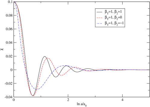
Figure 1: The evolutions of $\chi$ are plotted with different $\beta_{T}$ and $\beta_{2}$. We set to $\chi_{i}=0.1m_{pl}$

In order to preserve an isotropic background spacetime, we will use a timelike vector field ($\xi\equiv A_{\mu}A^{\mu}<0$) and then take as $A_{\mu}^{(0)}(t)=(A_{0}(t),\vec{0})\equiv(\chi(t),\vec{0})$. In the spatially flat FRW metric

$$ds^{2}=-dt^{2}+a^{2}(t)\gamma_{ij}dx^{i}dx^{j},$$ (10)

the field equation of $\chi$ and Einstein equations can be expressed as

$$\ddot{\chi} + 3H\dot{\chi}+\left[3\beta_{2}\dot{H}+3(\beta_{2}-\beta_{T})H^{2}+2\frac{dV}{d\xi}\right]\frac{1}{\beta_{T}}\chi=0,$$ (11)

$$\left(\frac{\dot{a}}{a}\right)^{2} = \frac{8\pi G}{3}\Biggl{[}-\beta_{T}(\chi\ddot{\chi}+\frac{1}{2}\dot{\chi}^{2}+3H\chi\dot{\chi}-\frac{3}{2}H^{2}\chi^{2})$$ (12)

$$~{}~{}~{}~{}-3\beta_{2}(H\chi\dot{\chi}+\dot{H}\chi^{2}+2H^{2}\chi^{2})+2\frac{dV}{d\xi}\chi^{2}+V\Biggr{]},$$

$$\dot{H} = 4\pi G\Biggl{[}(\beta_{T}-\beta_{2})(\chi\ddot{\chi}+\dot{\chi}^{2}+H\chi\dot{\chi}-\dot{H}\chi^{2}-3H^{2}\chi^{2})-2\frac{dV}{d\xi}\chi^{2}\Biggr{]}.$$ (13)

Here we have assumed $\beta_{T}\equiv\beta_{1}+\beta_{2}+\beta_{3}\neq 0$ for the timelike vector field to behave as a dynamical degree of freedom. The background evolutions of the vector field in (11), (12), and (13) are determined only by $\beta_{T}$ and $\beta_{2}$. This means that the models with the Lagrangian density (3) and (4) can not be distinguished from the background dynamics. In order to distinguish between these two models, we need to consider the linear perturbations. We plot the evolutions of the vector field with $\beta_{T}$ and $\beta_{2}$ for $V(\xi)=\frac{1}{2}m^{2}\xi$ in Fig. 1.

III Can inflation be possible?

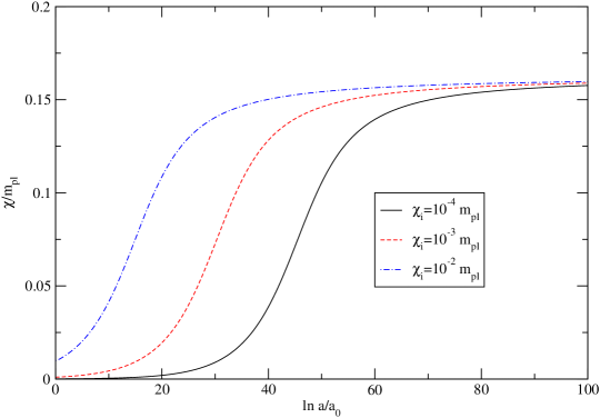
Figure 2: The evolutions of vector field are depicted depending on $\chi_{i}$ for $V=V_{0}-\frac{1}{2}m^{2}\xi$. We set to $\mu=m_{pl}$.

In this section, we check whether the timelike vector field can give rise to the period of inflationary expansion. In order to generate successful slow-roll inflation, slow-roll conditions ($\ddot{\chi}\ll 3H\dot{\chi}$, $\dot{\chi}^{2}/2\ll V(\xi)$ and $\dot{H}\ll H^{2}$) should be satisfied. From (11), we can define the effective mass of the vector field as

$$m_{eff}\equiv\frac{1}{\beta_{T}}\left(3\beta_{2}\dot{H}+3(\beta_{2}-\beta_{T})H^{2}+2\frac{dV}{d\xi}\right).$$ (14)

If we assume that the slow-roll conditions are satisfied, then $m_{eff}\simeq(3(\beta_{2}-\beta_{T})H^{2}+2dV/d\xi)/\beta_{T}$. In order for the vector field to roll slowly over the effective potential, $m_{eff}$ should be much smaller than $H^{2}$. But as long as $\beta_{T}\neq\beta_{2}$, $m_{eff}\sim H^{2}$ if $H^{2}\gg dV/d\xi$ or $m_{eff}\gg H^{2}$ if $H^{2}\ll dV/d\xi$. Only for $\beta_{T}=\beta_{2}$, there would be a possibility of $m_{eff}\ll H^{2}$ when $dV/d\xi\ll H^{2}$ is satisfied. Unless otherwise stated, we only focus on $\beta_{T}=\beta_{2}=1$ case in what follows.

In order to check the possibility of the inflationary expansion with the vector field, we require the following three minimal conditions one would expect a successful inflation model to satisfy: i)$H^{2}\propto\rho>0$ ii) $\ddot{a}/a\propto\rho+3P<0$ and iii) $|\dot{H}/H^{2}|\ll 1$. First condition is required in order to have a positive energy density, second is for an accelerating expansion and the final one is for slow-roll inflation. Then we could find a vector field potential to satisfy these conditions.

We can summarize the above three requirements as $\chi\ll m_{pl},~{}V+6(dV/d\xi)\chi^{2}>0$ and $(|dV/d\xi|)\chi^{2}\ll|V|$. With these conditions, $H^{2}\sim V$ and the number of efolds $N_{e}$ can be calculated as

$$N_{e}=\int Hdt=\int\frac{H}{\dot{\chi}}d\chi\sim\int\frac{4\pi V}{m_{pl}\chi|dV/d\xi|}d\chi.$$ (15)

We first consider the massive vector potential, $V=\frac{1}{2}m^{2}\xi=-\frac{1}{2}m^{2}\chi^{2}$, and apply the above conditions to this potential. Since $H^{2}\sim\dot{H}$ and $m_{eff}^{2}\sim H^{2}$ as shown in Ref. Koh:2009vm , this potential can not satisfy the slow-roll conditions and thus we can not obtain an accelerating expansion. We plot the evolution of the vector field with this massive potential in Fig. 1.

Next we consider the small field type potential as like in a scalar field inflation model

$$V=\lambda(\xi-\mu^{2})^{2}\simeq V_{0}-\frac{1}{2}m^{2}\xi,$$ (16)

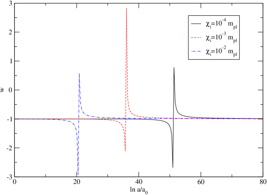
where $V_{0}=\lambda\mu^{4}$ and $m^{2}=4\lambda\mu^{2}$ and we have assumed $\chi\ll\mu$ in the last expression. This potential can satisfy all conditions as long as $\chi\ll\mu$. We plot the evolution of $\chi$ and equation of state parameter, $w=P/\rho$, with the initial conditions of $\chi$ for this potential in Figs. 2 and 3. $\chi_{i}$ can be constrained from $N_{e}$ which is required to be larger than $50$ in order to fit to the observations. But although the accelerating phase can occur, we need another mechanism to exit to the standard cosmology.

Figure 3: The evolutions of equation of state parameter, $w$, are depicted depending on $\chi_{i}$ for $V=V_{0}-\frac{1}{2}m^{2}\xi$.

IV Conclusion and discussion

We have investigated the vector field dynamics in the early universe and checked if the vector field can give rise to an inflationary expansion. In order to preserve an isotropic background spacetime, the timelike vector field is considered. The vector field potential is required to be $\rho>0,~{}\rho+3P<0$ and $|\dot{H}|\ll H^{2}$ in order to produce an inflationary expansion. The small field type potential as like in scalar driven inflation, $V\simeq V_{0}+\frac{1}{2}m^{2}\xi$, can give rise to an accelerating expansion and get a sufficient inflationary period by adjusting the initial condition of the field. However, there still seems to exist a problem to exit to the standard cosmology.

It would be interesting to calculate the scalar and tensor power spectrum and to compare with the observations. It is also needed to check the instability in sub-Hubble length scale with our model.

References

• (1) L. H. Ford, Phys. Rev.  D 40, 967 (1989).
• (2) A. Golovnev, V. Mukhanov and V. Vanchurin, JCAP 0806, 009 (2008) [arXiv:0802.2068 [astro-ph]].
• (3) S. Kanno, M. Kimura, J. Soda and S. Yokoyama, JCAP 0808, 034 (2008) [arXiv:0806.2422 [hep-ph]]; M. a. Watanabe, S. Kanno and J. Soda, arXiv:0902.2833 [hep-th].
• (4) C. Armendariz-Picon, JCAP 0407, 007 (2004) [arXiv:astro-ph/0405267]; J. B. Jimenez and A. L. Maroto, Phys. Rev.  D 78, 063005 (2008) [arXiv:0801.1486 [astro-ph]]; T. S. Koivisto and D. F. Mota, JCAP 0808, 021 (2008) [arXiv:0805.4229 [astro-ph]]; C. G. Boehmer and T. Harko, Eur. Phys. J.  C 50, 423 (2007) [arXiv:gr-qc/0701029]; K. Bamba, S. Nojiri and S. D. Odintsov, Phys. Rev.  D 77, 123532 (2008) [arXiv:0803.3384 [hep-th]].
• (5) B. Himmetoglu, C. R. Contaldi and M. Peloso, arXiv:0809.2779 [astro-ph]; B. Himmetoglu, C. R. Contaldi and M. Peloso, arXiv:0812.1231 [astro-ph].
• (6) S. M. Carroll, T. R. Dulaney, M. I. Gresham and H. Tam, arXiv:0812.1049 [hep-th].
• (7) S. Koh and B. Hu, arXiv:0901.0429 [hep-th].
• (8) T. Jacobson and D. Mattingly, Phys. Rev.  D 64, 024028 (2001) [arXiv:gr-qc/0007031]; S. M. Carroll and E. A. Lim, Phys. Rev.  D 70, 123525 (2004) [arXiv:hep-th/0407149].
• (9) L. Ford, private communication.
• (10) S. M. Carroll, T. R. Dulaney, M. I. Gresham and H. Tam, arXiv:0812.1050 [hep-th].
• (11) S. Koh, Work in porgress.