CMB Angular Power Spectrum from Correlated Primordial Fluctuation

B.Yu yubo@chenwang.nju.edu.cn Department of Physics, Nanjing University, Nanjing 210093, China    T.Lu t.lu@mail.pmo.ac.cn Purple Mountain Observatory, Chinese Academy of Sciences, Nanjing 210008, China Joint Center for Particle, Nuclear Physics and Cosmology, Nanjing University-Purple Mountain Observatory, Nanjing 210093, China
(.)
Abstract

The usual inflationary scenario predicts a Gaussian random primordial density fluctuation, different Fourier modes of which do not correlate with each other. In this paper we propose a correlation between these different modes. A simple case is that these different Fourier modes correlate with each other following a Gaussian function. For such a primordial density fluctuation we calculate the CMB angular power spectrum and find that its amplitude decreases but the decrease is different for different l𝑙l. This feature can be used to constrain the the correlation strength from the real data.

pacs:
98.70.Vc, 98.80.-k

I Introduction

In the inflationary scenario, the primordial fluctuation comes from the quantum vacuum fluctuation of the inflaton which drive the inflation Mukhanov and Chibisov (1981); Starobinsky (1982); Guth and Pi (1982); Hawking (1982). Then the quantum fluctuation becomes classical when the corresponding scale goes out of the horizon. The primordial fluctuation produced in this method is regarded to be Gaussian random and scale invariant, which are confirmed by many astronomical observations Smoot etΒ al. (1992); Bennett etΒ al. (1996); Spergel etΒ al. (2007); Hinshaw etΒ al. (2007).

This explanation of the origin of the primordial fluctuation seems reasonable and successful. However it is not a rigorous theory and needs more experimental tests. Besides the inflation, there exist other ideas to produce the primordial fluctuations, for example, the string gas model Nayeri etΒ al. (2006); Brandenberger etΒ al. (2007a, b); Brandenberger etΒ al. (2006). Even in the inflationary scenario, there are many kinds of modification to the primordial power spectrum, for example, the case that translational invariance is broken Carroll etΒ al. (2008) or rotational invariance is broken Ackerman etΒ al. (2007); Pullen and Kamionkowski (2007); Groeneboom and Eriksen (2009); Armendariz-Picon and Pekowsky (2008). The quantum-classical transition in the inflationary scenario is also criticized by Perez etΒ al. (2006). Considering these uncertainties, our paper is motivated by checking one of the main features of the Gaussian random fluctuation from the experiments: the different modes of the primordial fluctuation in the Fourier space are independent from each other. As we know, the Cosmic Microwave Background (CMB) is the relics of early universe, which can provide precise measurement on the primordial fluctuation. So in this paper we introduce a small correlation between different modes of the primordial fluctuation (in Fourier space) and then study how the correlation affects the CMB angular power spectrum.

This paper is organized as follows. In section II we introduce the above mentioned correlations of the primordial fluctuation in Fourier space. In section III we calculate the CMB angular power spectrum. The numerical results are presented in section IV and the discussions are given in section V.

II Primordial fluctuation

The meaning of the Gaussian random primordial density fluctuation is <ξ​(kβ†’)β€‹ΞΎβˆ—β€‹(kβ†’β€²)>=Ps​(k)​δ3​(kβ†’βˆ’kβ†’β€²)expectationπœ‰β†’π‘˜superscriptπœ‰superscriptβ†’π‘˜β€²superscriptπ‘ƒπ‘ π‘˜superscript𝛿3β†’π‘˜superscriptβ†’π‘˜β€²<\xi(\vec{k})\xi^{*}(\vec{k}^{{}^{\prime}})>=P^{s}(k)\delta^{3}(\vec{k}-\vec{k}^{{}^{\prime}}), where ξ​(kβ†’)πœ‰β†’π‘˜\xi(\vec{k}) is the Fourier mode of the primordial density fluctuation ξ​(xβ†’)πœ‰β†’π‘₯\xi(\vec{x}). The delta function indicates that different mode does not correlate with each other. One can relax this property by allowing different modes to correlate. Generally speaking, one can rewrite the above equation as <ξ​(kβ†’)β€‹ΞΎβˆ—β€‹(kβ†’β€²)>=f​(kβ†’,kβ†’β€²)expectationπœ‰β†’π‘˜superscriptπœ‰superscriptβ†’π‘˜β€²π‘“β†’π‘˜superscriptβ†’π‘˜β€²<\xi(\vec{k})\xi^{*}(\vec{k}^{{}^{\prime}})>=f(\vec{k},\vec{k}^{{}^{\prime}}), where f​(kβ†’,kβ†’β€²)π‘“β†’π‘˜superscriptβ†’π‘˜β€²f(\vec{k},\vec{k}^{{}^{\prime}}) is not required to be a delta function any more. However f​(kβ†’,kβ†’β€²)π‘“β†’π‘˜superscriptβ†’π‘˜β€²f(\vec{k},\vec{k}^{{}^{\prime}}) is not arbitrary, it must satisfy some constraints since ξ​(xβ†’)πœ‰β†’π‘₯\xi(\vec{x}) is a real field. <ξ​(kβ†’)β€‹ΞΎβˆ—β€‹(kβ†’β€²)>βˆ—=<ξ​(kβ†’β€²)β€‹ΞΎβˆ—β€‹(kβ†’)>superscriptexpectationπœ‰β†’π‘˜superscriptπœ‰superscriptβ†’π‘˜β€²expectationπœ‰superscriptβ†’π‘˜β€²superscriptπœ‰β†’π‘˜<\xi(\vec{k})\xi^{*}(\vec{k}^{{}^{\prime}})>^{*}=<\xi(\vec{k}^{{}^{\prime}})\xi^{*}(\vec{k})> gives fβˆ—β€‹(kβ†’,kβ†’β€²)=f​(kβ†’β€²,kβ†’)superscriptπ‘“β†’π‘˜superscriptβ†’π‘˜β€²π‘“superscriptβ†’π‘˜β€²β†’π‘˜f^{*}(\vec{k},\vec{k}^{{}^{\prime}})=f(\vec{k}^{{}^{\prime}},\vec{k}), which means the real part of f​(kβ†’,kβ†’β€²)π‘“β†’π‘˜superscriptβ†’π‘˜β€²f(\vec{k},\vec{k}^{{}^{\prime}}) is symmetric under the interchange of kβ†’,kβ†’β€²β†’π‘˜superscriptβ†’π‘˜β€²\vec{k},\vec{k}^{{}^{\prime}}, R​e​f​(kβ†’,kβ†’β€²)=R​e​f​(kβ†’β€²,kβ†’)π‘…π‘’π‘“β†’π‘˜superscriptβ†’π‘˜β€²π‘…π‘’π‘“superscriptβ†’π‘˜β€²β†’π‘˜Ref(\vec{k},\vec{k}^{{}^{\prime}})=Ref(\vec{k}^{{}^{\prime}},\vec{k}), and the imaginary part of f​(kβ†’,kβ†’β€²)π‘“β†’π‘˜superscriptβ†’π‘˜β€²f(\vec{k},\vec{k}^{{}^{\prime}}) is antisymmetric under the interchange of kβ†’,kβ†’β€²β†’π‘˜superscriptβ†’π‘˜β€²\vec{k},\vec{k}^{{}^{\prime}}, I​m​f​(kβ†’,kβ†’β€²)=βˆ’I​m​f​(kβ†’β€²,kβ†’)πΌπ‘šπ‘“β†’π‘˜superscriptβ†’π‘˜β€²πΌπ‘šπ‘“superscriptβ†’π‘˜β€²β†’π‘˜Imf(\vec{k},\vec{k}^{{}^{\prime}})=-Imf(\vec{k}^{{}^{\prime}},\vec{k}). Besides this, ΞΎβˆ—β€‹(kβ†’)=ξ​(βˆ’kβ†’)superscriptπœ‰β†’π‘˜πœ‰β†’π‘˜\xi^{*}(\vec{k})=\xi(-\vec{k}), which indicates that <ΞΎβˆ—β€‹(βˆ’kβ†’)​ξ​(βˆ’kβ†’β€²)>=f​(βˆ’kβ†’β€²,βˆ’kβ†’)=f​(kβ†’,kβ†’β€²)=<ξ​(kβ†’)β€‹ΞΎβˆ—β€‹(kβ†’β€²)>expectationsuperscriptπœ‰β†’π‘˜πœ‰superscriptβ†’π‘˜β€²π‘“superscriptβ†’π‘˜β€²β†’π‘˜π‘“β†’π‘˜superscriptβ†’π‘˜β€²expectationπœ‰β†’π‘˜superscriptπœ‰superscriptβ†’π‘˜β€²<\xi^{*}(-\vec{k})\xi(-\vec{k}^{{}^{\prime}})>=f(-\vec{k}^{{}^{\prime}},-\vec{k})=f(\vec{k},\vec{k}^{{}^{\prime}})=<\xi(\vec{k})\xi^{*}(\vec{k}^{{}^{\prime}})>. Thus one obtains R​e​f​(βˆ’kβ†’,βˆ’kβ†’β€²)=R​e​f​(βˆ’kβ†’β€²,βˆ’kβ†’)=R​e​f​(kβ†’,kβ†’β€²)π‘…π‘’π‘“β†’π‘˜superscriptβ†’π‘˜β€²π‘…π‘’π‘“superscriptβ†’π‘˜β€²β†’π‘˜π‘…π‘’π‘“β†’π‘˜superscriptβ†’π‘˜β€²Ref(-\vec{k},-\vec{k}^{{}^{\prime}})=Ref(-\vec{k}^{{}^{\prime}},-\vec{k})=Ref(\vec{k},\vec{k}^{{}^{\prime}}) and I​m​f​(βˆ’kβ†’,βˆ’kβ†’β€²)=βˆ’I​m​f​(βˆ’kβ†’β€²,βˆ’kβ†’)=βˆ’I​m​f​(kβ†’,kβ†’β€²)πΌπ‘šπ‘“β†’π‘˜superscriptβ†’π‘˜β€²πΌπ‘šπ‘“superscriptβ†’π‘˜β€²β†’π‘˜πΌπ‘šπ‘“β†’π‘˜superscriptβ†’π‘˜β€²Imf(-\vec{k},-\vec{k}^{{}^{\prime}})=-Imf(-\vec{k}^{{}^{\prime}},-\vec{k})=-Imf(\vec{k},\vec{k}^{{}^{\prime}}). Ps​(k)​δ3​(kβ†’βˆ’kβ†’β€²)superscriptπ‘ƒπ‘ π‘˜superscript𝛿3β†’π‘˜superscriptβ†’π‘˜β€²P^{s}(k)\delta^{3}(\vec{k}-\vec{k}^{{}^{\prime}}) is such a special function with a zero imaginary part.

However, these constraints provide no positive information on the function f​(kβ†’,kβ†’β€²)π‘“β†’π‘˜superscriptβ†’π‘˜β€²f(\vec{k},\vec{k}^{{}^{\prime}}). We must construct a concrete form of the above function. It is not strange to require that delta function is a good approximation to this function, and noting that when Οƒβ†’0β†’πœŽ0\sigma\rightarrow 0, 12​π​σ​exp⁑[βˆ’(xβˆ’y)22​σ]→δ​(xβˆ’y)β†’12πœ‹πœŽsuperscriptπ‘₯𝑦22πœŽπ›Ώπ‘₯𝑦\frac{1}{\sqrt{2\pi\sigma}}\exp{[-\frac{(x-y)^{2}}{2\sigma}]}\rightarrow\delta(x-y), one can use a very simple form

(12​π​σ0​ko2)3​exp⁑[βˆ’(kβ†’βˆ’kβ†’β€²)22​σ0​ko2]superscript12πœ‹subscript𝜎0subscriptsuperscriptπ‘˜2π‘œ3superscriptβ†’π‘˜superscriptβ†’π‘˜β€²22subscript𝜎0subscriptsuperscriptπ‘˜2π‘œ\displaystyle(\frac{1}{\sqrt{2\pi\sigma_{0}k^{2}_{o}}})^{3}\exp{[-\frac{(\vec{k}-\vec{k}^{{}^{\prime}})^{2}}{2\sigma_{0}k^{2}_{o}}]} (1)

to replace the delta function. When Οƒ0β†’0β†’subscript𝜎00\sigma_{0}\rightarrow 0, it approaches Ξ΄3​(kβ†’βˆ’kβ†’β€²)superscript𝛿3β†’π‘˜superscriptβ†’π‘˜β€²\delta^{3}(\vec{k}-\vec{k}^{{}^{\prime}}). Here Οƒ0subscript𝜎0\sigma_{0} is a pure number and k0subscriptπ‘˜0k_{0} is the comoving wave number. This is a Gaussian form function, which is completely determined by the parameter σ≑σ0​k02𝜎subscript𝜎0subscriptsuperscriptπ‘˜20\sigma\equiv\sigma_{0}k^{2}_{0} and its maximum is located at kβ†’=kβ†’β€²β†’π‘˜superscriptβ†’π‘˜β€²\vec{k}=\vec{k}^{{}^{\prime}}. The FWHM is 2​2​ln⁑2​σ222𝜎2\sqrt{2\ln 2\sigma}. Then in order to satisfy the above constraints, one can generalize Ps​(k)superscriptπ‘ƒπ‘ π‘˜P^{s}(k) to Ps​(k​kβ€²)superscriptπ‘ƒπ‘ π‘˜superscriptπ‘˜β€²P^{s}(\sqrt{kk^{{}^{\prime}}}) or Ps​(k+kβ€²2)superscriptπ‘ƒπ‘ π‘˜superscriptπ‘˜β€²2P^{s}(\frac{k+k^{{}^{\prime}}}{2}). Their difference can be ignored in the weak correlation case (ΟƒπœŽ\sigma is small), but cannot be ignored in the strong correlation case (ΟƒπœŽ\sigma is great). However, it is easy to note that the strong correlation case is excluded by the CMB observation, so in this paper we only take

f​(kβ†’,kβ†’β€²)=Ps​(k+kβ€²2)​(12​π​σ0​ko2)3​exp⁑[βˆ’(kβ†’βˆ’kβ†’β€²)22​σ0​ko2]π‘“β†’π‘˜superscriptβ†’π‘˜β€²superscriptπ‘ƒπ‘ π‘˜superscriptπ‘˜β€²2superscript12πœ‹subscript𝜎0subscriptsuperscriptπ‘˜2π‘œ3superscriptβ†’π‘˜superscriptβ†’π‘˜β€²22subscript𝜎0subscriptsuperscriptπ‘˜2π‘œ\displaystyle f(\vec{k},\vec{k}^{{}^{\prime}})=P^{s}(\frac{k+k^{{}^{\prime}}}{2})(\frac{1}{\sqrt{2\pi\sigma_{0}k^{2}_{o}}})^{3}\exp{[-\frac{(\vec{k}-\vec{k}^{{}^{\prime}})^{2}}{2\sigma_{0}k^{2}_{o}}]} (2)

as an example to study the correlation effects on CMB angular power spectrum. In fact, the following discussions not only apply to primordial fluctuation with form (2) but also to such a form f​(kβ†’,kβ†’β€²)=f​(k,kβ€²,|kβ†’βˆ’kβ†’β€²|)π‘“β†’π‘˜superscriptβ†’π‘˜β€²π‘“π‘˜superscriptπ‘˜β€²β†’π‘˜superscriptβ†’π‘˜β€²f(\vec{k},\vec{k}^{{}^{\prime}})=f(k,k^{{}^{\prime}},|\vec{k}-\vec{k}^{{}^{\prime}}|). It can be rewritten as

f​(k,kβ€²,|kβ†’βˆ’kβ†’β€²|)=∫d3​Δ→​f​(k,kβ€²,|Ξ”β†’|)​δ3​(kβ†’βˆ’kβ†’β€²βˆ’Ξ”β†’)π‘“π‘˜superscriptπ‘˜β€²β†’π‘˜superscriptβ†’π‘˜β€²superscript𝑑3β†’Ξ”π‘“π‘˜superscriptπ‘˜β€²β†’Ξ”superscript𝛿3β†’π‘˜superscriptβ†’π‘˜β€²β†’Ξ”\displaystyle f(k,k^{{}^{\prime}},|\vec{k}-\vec{k}^{{}^{\prime}}|)=\int d^{3}\vec{\Delta}f(k,k^{{}^{\prime}},|\vec{\Delta}|)\delta^{3}(\vec{k}-\vec{k}^{{}^{\prime}}-\vec{\Delta}) (3)

III CMB Power Spectrum

III.1 Two point correlator

For scalar type of primordial density fluctuation, the CMB temperature anisotropy at direction n→→𝑛\vec{n} can be expressed as Dodelson ; Zaldarriaga and Seljak (1997)

Ts​(nβ†’)superscript𝑇𝑠→𝑛\displaystyle T^{s}(\vec{n}) =\displaystyle= ∫d3​k→​ΔTs​(Ξ·0,k,k^β‹…n^)​ξ​(kβ†’)superscript𝑑3β†’π‘˜subscriptsuperscriptΔ𝑠𝑇subscriptπœ‚0π‘˜β‹…^π‘˜^π‘›πœ‰β†’π‘˜\displaystyle\int d^{3}\vec{k}\Delta^{s}_{T}(\eta_{0},k,\hat{k}\cdot\hat{n})\xi(\vec{k}) (4)
=\displaystyle= ∫d3​kβ†’β€‹βˆ«0Ξ·0𝑑η​STs​(Ξ·,k)​eβˆ’i​x​k^β‹…n^​ξ​(kβ†’)superscript𝑑3β†’π‘˜subscriptsuperscriptsubscriptπœ‚00differential-dπœ‚superscriptsubscriptπ‘†π‘‡π‘ πœ‚π‘˜superscript𝑒⋅𝑖π‘₯^π‘˜^π‘›πœ‰β†’π‘˜\displaystyle\int d^{3}\vec{k}\int^{\eta_{0}}_{0}d\eta S_{T}^{s}(\eta,k)e^{-ix\hat{k}\cdot\hat{n}}\xi(\vec{k})

where STs​(Ξ·,k)superscriptsubscriptπ‘†π‘‡π‘ πœ‚π‘˜S_{T}^{s}(\eta,k) is the transfer function, x≑k​(Ξ·0βˆ’Ξ·)π‘₯π‘˜subscriptπœ‚0πœ‚x\equiv k(\eta_{0}-\eta), Ξ·πœ‚\eta is the conformal time and Ξ·0subscriptπœ‚0\eta_{0} is the conformal time of today. Following the standard methods, the temperature anisotropy can be expanded by the spherical harmonic coefficients

al​m=βˆ«π‘‘Ξ©β€‹Yl​mβˆ—β€‹(nβ†’)​Ts​(nβ†’).subscriptπ‘Žπ‘™π‘šdifferential-dΞ©superscriptsubscriptπ‘Œπ‘™π‘šβ†’π‘›superscript𝑇𝑠→𝑛\displaystyle a_{lm}=\int d\Omega Y_{lm}^{*}(\vec{n})T^{s}(\vec{n}). (5)

An important property of the modified primordial power spectrum <ξ​(kβ†’)β€‹ΞΎβˆ—β€‹(kβ†’β€²)>=f​(k,kβ€²,|kβ†’βˆ’kβ†’β€²|)expectationπœ‰β†’π‘˜superscriptπœ‰superscriptβ†’π‘˜β€²π‘“π‘˜superscriptπ‘˜β€²β†’π‘˜superscriptβ†’π‘˜β€²<\xi(\vec{k})\xi^{*}(\vec{k}^{{}^{\prime}})>=f(k,k^{{}^{\prime}},|\vec{k}-\vec{k}^{{}^{\prime}}|) is that the CMB anisotropy produced by such a form of primordial density fluctuation is statistically rotational invariant which means that for any rotation R𝑅R one always have

<Ts​(R​nβ†’β€²)​Ts​(R​nβ†’)>=<Ts​(nβ†’β€²)​Ts​(nβ†’)>.expectationsuperscript𝑇𝑠𝑅superscript→𝑛′superscript𝑇𝑠𝑅→𝑛expectationsuperscript𝑇𝑠superscript→𝑛′superscript𝑇𝑠→𝑛\displaystyle<T^{s}(R\vec{n}^{{}^{\prime}})T^{s}(R\vec{n})>=<T^{s}(\vec{n}^{{}^{\prime}})T^{s}(\vec{n})>. (6)

The definite proof of Eq.(6) is postponed to Appendix. With this property, one can obtain the following conclusion Hu (2001)

<al​m​al′​mβ€²βˆ—>=Ξ΄l​l′​δm​m′​Cl.expectationsubscriptπ‘Žπ‘™π‘šsubscriptsuperscriptπ‘Žsuperscript𝑙′superscriptπ‘šβ€²subscript𝛿𝑙superscript𝑙′subscriptπ›Ώπ‘šsuperscriptπ‘šβ€²subscript𝐢𝑙\displaystyle<a_{lm}a^{*}_{l^{{}^{\prime}}m^{{}^{\prime}}}>=\delta_{ll^{{}^{\prime}}}\delta_{mm^{{}^{\prime}}}C_{l}. (7)

So the angular power spectrum Clsubscript𝐢𝑙C_{l} is sufficient to reflect all the two point correlators of CMB anisotropy.

III.2 Power spectrum

The CMB angular power spectrum can be calculated by

Clsubscript𝐢𝑙\displaystyle C_{l} =\displaystyle= 12​l+1β€‹βˆ‘m<al​mβˆ—β€‹al​m>12𝑙1subscriptπ‘šexpectationsubscriptsuperscriptπ‘Žπ‘™π‘šsubscriptπ‘Žπ‘™π‘š\displaystyle\dfrac{1}{2l+1}\sum_{m}<a^{*}_{lm}a_{lm}> (8)
=\displaystyle= 12​l+1β€‹βˆ‘m<(βˆ«π‘‘Ξ©β€‹Yl​mβˆ—β€‹(nβ†’β€²)​T​(nβ†’β€²))βˆ—12𝑙1subscriptπ‘šsuperscriptdifferential-dΞ©superscriptsubscriptπ‘Œπ‘™π‘šsuperscript→𝑛′𝑇superscript→𝑛′\displaystyle\dfrac{1}{2l+1}\sum_{m}<(\int d\Omega Y_{lm}^{*}(\vec{n}^{{}^{\prime}})T(\vec{n}^{{}^{\prime}}))^{*}
(βˆ«π‘‘Ξ©β€‹Yl​mβˆ—β€‹(nβ†’)​T​(nβ†’))>differential-dΞ©superscriptsubscriptπ‘Œπ‘™π‘šβ†’π‘›π‘‡β†’π‘›absent\displaystyle(\int d\Omega Y_{lm}^{*}(\vec{n})T(\vec{n}))>

Substituting Eq.(4) into Eq.(8), one obtains

Cl=subscript𝐢𝑙absent\displaystyle C_{l}= (4​π)22​l+1β€‹βˆ‘m∫d3​k→′​d3​k→​Gl​(kβ€²)​Gl​(k)superscript4πœ‹22𝑙1subscriptπ‘šsuperscript𝑑3superscriptβ†’π‘˜β€²superscript𝑑3β†’π‘˜subscript𝐺𝑙superscriptπ‘˜β€²subscriptπΊπ‘™π‘˜\displaystyle\dfrac{(4\pi)^{2}}{2l+1}\sum_{m}\int d^{3}\vec{k}^{{}^{\prime}}d^{3}\vec{k}G_{l}(k^{{}^{\prime}})G_{l}(k)
Yl​m​(k^β€²)​Yl​mβˆ—β€‹(k^)​<ξ​(kβ†’)β€‹ΞΎβˆ—β€‹(kβ†’β€²)>subscriptπ‘Œπ‘™π‘šsuperscript^π‘˜β€²superscriptsubscriptπ‘Œπ‘™π‘š^π‘˜expectationπœ‰β†’π‘˜superscriptπœ‰superscriptβ†’π‘˜β€²\displaystyle Y_{lm}(\hat{k}^{{}^{\prime}})Y_{lm}^{*}(\hat{k})<\xi(\vec{k})\xi^{*}(\vec{k}^{{}^{\prime}})>
=\displaystyle= ∫d3​Δ→​F​(Ξ”β†’),superscript𝑑3→Δ𝐹→Δ\displaystyle\int d^{3}\vec{\Delta}F(\vec{\Delta}), (9)

where the formula ei​kβ†’β‹…xβ†’=4β€‹Ο€β€‹βˆ‘l​mil​jl​(k​x)​Yl​mβˆ—β€‹(k^)​Yl​m​(x^)superscripteβ‹…π‘–β†’π‘˜β†’π‘₯4πœ‹subscriptπ‘™π‘šsuperscript𝑖𝑙subscriptπ‘—π‘™π‘˜π‘₯subscriptsuperscriptπ‘Œπ‘™π‘š^π‘˜subscriptπ‘Œπ‘™π‘š^π‘₯{\rm e}^{i\vec{k}\cdotp\vec{x}}=4\pi\sum_{lm}i^{l}j_{l}(kx)Y^{*}_{lm}(\hat{k})Y_{lm}(\hat{x}) has been used and F​(Ξ”β†’)𝐹→ΔF(\vec{\Delta}) is defined by

F​(Ξ”β†’)𝐹→Δ\displaystyle F(\vec{\Delta}) ≑\displaystyle\equiv (4​π)22​l+1β€‹βˆ‘m∫d3​k→′​d3​k→​Gl​(kβ€²)​Gl​(k)​Yl​m​(k^β€²)superscript4πœ‹22𝑙1subscriptπ‘šsuperscript𝑑3superscriptβ†’π‘˜β€²superscript𝑑3β†’π‘˜subscript𝐺𝑙superscriptπ‘˜β€²subscriptπΊπ‘™π‘˜subscriptπ‘Œπ‘™π‘šsuperscript^π‘˜β€²\displaystyle\dfrac{(4\pi)^{2}}{2l+1}\sum_{m}\int d^{3}\vec{k}^{{}^{\prime}}d^{3}\vec{k}G_{l}(k^{{}^{\prime}})G_{l}(k)Y_{lm}(\hat{k}^{{}^{\prime}}) (10)
Yl​mβˆ—β€‹(k^)​f​(k,kβ€²,|Ξ”β†’|)​δ3​(kβ†’βˆ’kβ†’β€²βˆ’Ξ”β†’),superscriptsubscriptπ‘Œπ‘™π‘š^π‘˜π‘“π‘˜superscriptπ‘˜β€²β†’Ξ”superscript𝛿3β†’π‘˜superscriptβ†’π‘˜β€²β†’Ξ”\displaystyle Y_{lm}^{*}(\hat{k})f(k,k^{{}^{\prime}},|\vec{\Delta}|)\delta^{3}(\vec{k}-\vec{k}^{{}^{\prime}}-\vec{\Delta}),

where Gl​(k)β‰‘βˆ«0Ξ·0𝑑η​STs​(Ξ·,k)​jl​(x)subscriptπΊπ‘™π‘˜subscriptsuperscriptsubscriptπœ‚00differential-dπœ‚superscriptsubscriptπ‘†π‘‡π‘ πœ‚π‘˜subscript𝑗𝑙π‘₯G_{l}(k)\equiv\int^{\eta_{0}}_{0}d\eta S_{T}^{s}(\eta,k)j_{l}(x). In the Appendix we have proved

F​(R​Δ→)=F​(Ξ”β†’).𝐹𝑅→Δ𝐹→Δ\displaystyle F(R\vec{\Delta})=F(\vec{\Delta}). (11)

So, F​(Ξ”β†’)𝐹→ΔF(\vec{\Delta}) is only a function of Δ≑|Ξ”β†’|Ξ”β†’Ξ”\Delta\equiv|\vec{\Delta}|. Thus

Cl=4β€‹Ο€β€‹βˆ«0βˆžΞ”2​𝑑Δ​F​(Ξ”).subscript𝐢𝑙4πœ‹subscriptsuperscript0superscriptΞ”2differential-dΔ𝐹Δ\displaystyle C_{l}=4\pi\int^{\infty}_{0}\Delta^{2}d\Delta F(\Delta). (12)

Introducing new variables pβ†’=kβ†’+kβ†’β€²,pβ†’=kβ†’βˆ’kβ†’β€²formulae-sequenceβ†’π‘β†’π‘˜superscriptβ†’π‘˜β€²β†’π‘β†’π‘˜superscriptβ†’π‘˜β€²\vec{p}=\vec{k}+\vec{k}^{{}^{\prime}},\vec{p}=\vec{k}-\vec{k}^{{}^{\prime}}, and |βˆ‚(kβ†’,kβ†’β€²)βˆ‚(pβ†’,pβ†’β€²)|=18β†’π‘˜superscriptβ†’π‘˜β€²β†’π‘superscript→𝑝′18|\dfrac{\partial(\vec{k},\vec{k}^{{}^{\prime}})}{\partial(\vec{p},\vec{p}^{{}^{\prime}})}|=\frac{1}{8}, one obtains

F​(Ξ”β†’)𝐹→Δ\displaystyle F(\vec{\Delta}) =\displaystyle= (4​π)28​(2​l+1)β€‹βˆ‘m∫d3​p→​d3​p→′​Gl​(kβ€²)​Gl​(k)​Yl​m​(k^β€²)superscript4πœ‹282𝑙1subscriptπ‘šsuperscript𝑑3→𝑝superscript𝑑3superscript→𝑝′subscript𝐺𝑙superscriptπ‘˜β€²subscriptπΊπ‘™π‘˜subscriptπ‘Œπ‘™π‘šsuperscript^π‘˜β€²\displaystyle\dfrac{(4\pi)^{2}}{8(2l+1)}\sum_{m}\int d^{3}\vec{p}d^{3}\vec{p}^{{}^{\prime}}G_{l}(k^{{}^{\prime}})G_{l}(k)Y_{lm}(\hat{k}^{{}^{\prime}}) (13)
Yl​mβˆ—β€‹(k^)​f​(k,kβ€²,|Ξ”β†’|)​δ3​(pβ†’β€²βˆ’Ξ”β†’)superscriptsubscriptπ‘Œπ‘™π‘š^π‘˜π‘“π‘˜superscriptπ‘˜β€²β†’Ξ”superscript𝛿3superscript→𝑝′→Δ\displaystyle Y_{lm}^{*}(\hat{k})f(k,k^{{}^{\prime}},|\vec{\Delta}|)\delta^{3}(\vec{p}^{{}^{\prime}}-\vec{\Delta})
=\displaystyle= (4​π)28​(2​l+1)β€‹βˆ‘m∫d3​p→​Gl​(kβ€²)​Gl​(k)​Yl​m​(k^β€²)superscript4πœ‹282𝑙1subscriptπ‘šsuperscript𝑑3→𝑝subscript𝐺𝑙superscriptπ‘˜β€²subscriptπΊπ‘™π‘˜subscriptπ‘Œπ‘™π‘šsuperscript^π‘˜β€²\displaystyle\dfrac{(4\pi)^{2}}{8(2l+1)}\sum_{m}\int d^{3}\vec{p}G_{l}(k^{{}^{\prime}})G_{l}(k)Y_{lm}(\hat{k}^{{}^{\prime}})
Yl​mβˆ—β€‹(k^)​f​(k,kβ€²,Ξ”)superscriptsubscriptπ‘Œπ‘™π‘š^π‘˜π‘“π‘˜superscriptπ‘˜β€²Ξ”\displaystyle Y_{lm}^{*}(\hat{k})f(k,k^{{}^{\prime}},\Delta)
=\displaystyle= Ο€2β€‹βˆ«d3​p→​Gl​(kβ€²)​Gl​(k)​Pl​(kβ€²^β‹…k^)​f​(k,kβ€²,Ξ”),πœ‹2superscript𝑑3→𝑝subscript𝐺𝑙superscriptπ‘˜β€²subscriptπΊπ‘™π‘˜subscript𝑃𝑙⋅^superscriptπ‘˜β€²^π‘˜π‘“π‘˜superscriptπ‘˜β€²Ξ”\displaystyle\dfrac{\pi}{2}\int d^{3}\vec{p}G_{l}(k^{{}^{\prime}})G_{l}(k)P_{l}(\hat{k^{{}^{\prime}}}\cdot\hat{k})f(k,k^{{}^{\prime}},\Delta),

where kβ†’=pβ†’+pβ†’β€²2,kβ†’=pβ†’βˆ’pβ†’β€²2formulae-sequenceβ†’π‘˜β†’π‘superscript→𝑝′2β†’π‘˜β†’π‘superscript→𝑝′2\vec{k}=\dfrac{\vec{p}+\vec{p}^{{}^{\prime}}}{2},\vec{k}=\dfrac{\vec{p}-\vec{p}^{{}^{\prime}}}{2}. Since F​(Ξ”β†’)𝐹→ΔF(\vec{\Delta}) is only a function of ΔΔ\Delta, one can safely set Ξ”β†’β†’Ξ”\vec{\Delta} in the z𝑧z direction Ξ”β†’=Δ​ez→→ΔΔ→subscript𝑒𝑧\vec{\Delta}=\Delta\vec{e_{z}}, then k=px2+py2+(pz+Ξ”)22π‘˜superscriptsubscript𝑝π‘₯2superscriptsubscript𝑝𝑦2superscriptsubscript𝑝𝑧Δ22k=\dfrac{\sqrt{p_{x}^{2}+p_{y}^{2}+(p_{z}+\Delta)^{2}}}{2}, kβ€²=px2+py2+(pzβˆ’Ξ”)22superscriptπ‘˜β€²superscriptsubscript𝑝π‘₯2superscriptsubscript𝑝𝑦2superscriptsubscript𝑝𝑧Δ22k^{{}^{\prime}}=\dfrac{\sqrt{p_{x}^{2}+p_{y}^{2}+(p_{z}-\Delta)^{2}}}{2}, kβ€²^β‹…k^=px2+py2+pz2βˆ’Ξ”24​k​kβ€²β‹…^superscriptπ‘˜β€²^π‘˜superscriptsubscript𝑝π‘₯2superscriptsubscript𝑝𝑦2superscriptsubscript𝑝𝑧2superscriptΞ”24π‘˜superscriptπ‘˜β€²\hat{k^{{}^{\prime}}}\cdot\hat{k}=\dfrac{p_{x}^{2}+p_{y}^{2}+p_{z}^{2}-\Delta^{2}}{4kk^{{}^{\prime}}}. Noting that the integrand is only a function of px2+py2superscriptsubscript𝑝π‘₯2superscriptsubscript𝑝𝑦2p_{x}^{2}+p_{y}^{2}, and using

βˆ«βˆ’βˆž+βˆžπ‘‘pxβ€‹βˆ«βˆ’βˆž+βˆžπ‘‘py​f​(px2+py2)superscriptsubscriptdifferential-dsubscript𝑝π‘₯superscriptsubscriptdifferential-dsubscript𝑝𝑦𝑓superscriptsubscript𝑝π‘₯2superscriptsubscript𝑝𝑦2\displaystyle\int_{-\infty}^{+\infty}dp_{x}\int_{-\infty}^{+\infty}dp_{y}f(p_{x}^{2}+p_{y}^{2}) (14)
=\displaystyle= ∫0∞p¯​𝑑pΒ―β€‹βˆ«0π𝑑θ​f​(pΒ―2)subscriptsuperscript0¯𝑝differential-d¯𝑝subscriptsuperscriptπœ‹0differential-dπœƒπ‘“superscript¯𝑝2\displaystyle\int^{\infty}_{0}\bar{p}d\bar{p}\int^{\pi}_{0}d\theta f(\bar{p}^{2})
=\displaystyle= 2β€‹Ο€β€‹βˆ«0∞p¯​𝑑p¯​f​(pΒ―2),2πœ‹subscriptsuperscript0¯𝑝differential-d¯𝑝𝑓superscript¯𝑝2\displaystyle 2\pi\int^{\infty}_{0}\bar{p}d\bar{p}f(\bar{p}^{2}),

one obtains

Cl=subscript𝐢𝑙absent\displaystyle C_{l}= 4​π3β€‹βˆ«0βˆžΞ”2β€‹π‘‘Ξ”β€‹βˆ«βˆ’βˆž+βˆžπ‘‘pzβ€‹βˆ«0∞p¯​𝑑p¯​Gl​(kβ€²)​Gl​(k)4superscriptπœ‹3subscriptsuperscript0superscriptΞ”2differential-dΞ”subscriptsuperscriptdifferential-dsubscript𝑝𝑧subscriptsuperscript0¯𝑝differential-d¯𝑝subscript𝐺𝑙superscriptπ‘˜β€²subscriptπΊπ‘™π‘˜\displaystyle 4\pi^{3}\int^{\infty}_{0}\Delta^{2}d\Delta\int^{+\infty}_{-\infty}dp_{z}\int^{\infty}_{0}\bar{p}d\bar{p}G_{l}(k^{{}^{\prime}})G_{l}(k) (15)
Pl​(kβ€²^β‹…k^)​f​(k,kβ€²,Ξ”).subscript𝑃𝑙⋅^superscriptπ‘˜β€²^π‘˜π‘“π‘˜superscriptπ‘˜β€²Ξ”\displaystyle P_{l}(\hat{k^{{}^{\prime}}}\cdot\hat{k})f(k,k^{{}^{\prime}},\Delta).

Finally noting that the integrand is an even function of pzsubscript𝑝𝑧p_{z}, one obtains a simple form,

Clsubscript𝐢𝑙\displaystyle C_{l} =\displaystyle= Ο€2​(4​π)2β€‹βˆ«0βˆžΞ”2β€‹π‘‘Ξ”β€‹βˆ«0βˆžπ‘‘pzβ€‹βˆ«0∞p¯​𝑑pΒ―πœ‹2superscript4πœ‹2subscriptsuperscript0superscriptΞ”2differential-dΞ”subscriptsuperscript0differential-dsubscript𝑝𝑧subscriptsuperscript0¯𝑝differential-d¯𝑝\displaystyle\frac{\pi}{2}(4\pi)^{2}\int^{\infty}_{0}\Delta^{2}d\Delta\int^{\infty}_{0}dp_{z}\int^{\infty}_{0}\bar{p}d\bar{p} (16)
Gl​(kβ€²)​Gl​(k)​Pl​(kβ€²^β‹…k^)​f​(k,kβ€²,Ξ”),subscript𝐺𝑙superscriptπ‘˜β€²subscriptπΊπ‘™π‘˜subscript𝑃𝑙⋅^superscriptπ‘˜β€²^π‘˜π‘“π‘˜superscriptπ‘˜β€²Ξ”\displaystyle G_{l}(k^{{}^{\prime}})G_{l}(k)P_{l}(\hat{k^{{}^{\prime}}}\cdot\hat{k})f(k,k^{{}^{\prime}},\Delta),

where Gl​(k)β‰‘βˆ«0Ξ·0𝑑η​STs​(Ξ·,k)​jl​(x)subscriptπΊπ‘™π‘˜subscriptsuperscriptsubscriptπœ‚00differential-dπœ‚superscriptsubscriptπ‘†π‘‡π‘ πœ‚π‘˜subscript𝑗𝑙π‘₯G_{l}(k)\equiv\int^{\eta_{0}}_{0}d\eta S_{T}^{s}(\eta,k)j_{l}(x), k=pΒ―2+(pz+Ξ”)22π‘˜superscript¯𝑝2superscriptsubscript𝑝𝑧Δ22k=\dfrac{\sqrt{\bar{p}^{2}+(p_{z}+\Delta)^{2}}}{2}, kβ€²=pΒ―2+(pzβˆ’Ξ”)22superscriptπ‘˜β€²superscript¯𝑝2superscriptsubscript𝑝𝑧Δ22k^{{}^{\prime}}=\dfrac{\sqrt{\bar{p}^{2}+(p_{z}-\Delta)^{2}}}{2} and kβ€²^β‹…k^=pΒ―2+pz2βˆ’Ξ”24​k​kβ€²β‹…^superscriptπ‘˜β€²^π‘˜superscript¯𝑝2superscriptsubscript𝑝𝑧2superscriptΞ”24π‘˜superscriptπ‘˜β€²\hat{k^{{}^{\prime}}}\cdot\hat{k}=\dfrac{\bar{p}^{2}+p_{z}^{2}-\Delta^{2}}{4kk^{{}^{\prime}}}.

IV Numerical Results

In this paper we use the Boltzmann code CMBFAST (Seljak and Zaldarriaga (1996)) to do numerical calculation and adopt a flat Λ​C​D​MΛ𝐢𝐷𝑀\Lambda CDM model with cosmological parameters: Ξ©b=0.045subscriptΩ𝑏0.045\Omega_{b}=0.045, Ξ©c=0.225subscriptΩ𝑐0.225\Omega_{c}=0.225, ΩΛ=0.73subscriptΩΛ0.73\Omega_{\Lambda}=0.73, H0=70subscript𝐻070H_{0}=70, Ο„=0.08𝜏0.08\tau=0.08, ns=1subscript𝑛𝑠1n_{s}=1 and Δξ2=1subscriptsuperscriptΞ”2πœ‰1\Delta^{2}_{\xi}=1. Where Ο„πœ\tau is the optical depth, nssubscript𝑛𝑠n_{s} is spectral index and ΔξsubscriptΞ”πœ‰\Delta_{\xi} is the primordial scalar perturbation amplitude. In CMB power spectrum calculation Δξ2subscriptsuperscriptΞ”2πœ‰\Delta^{2}_{\xi} is only a normalization factor, the value of which is determined by observational data. Thus we can safely set it to be unit (usually the value of Δξ2subscriptsuperscriptΞ”2πœ‰\Delta^{2}_{\xi} is taken to be about 2.35Γ—10βˆ’102.35superscript10102.35\times 10^{-10}), which will not affect the following discussion, since we mainly care about the relative change of the power spectrum.

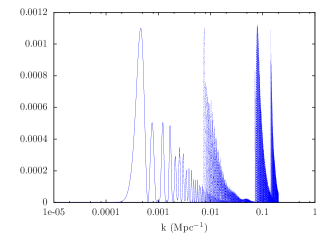
First we calculate (Gl​(k))2=(∫0Ξ·0𝑑η​STs​(Ξ·,k)​jl​(x))2superscriptsubscriptπΊπ‘™π‘˜2superscriptsubscriptsuperscriptsubscriptπœ‚00differential-dπœ‚superscriptsubscriptπ‘†π‘‡π‘ πœ‚π‘˜subscript𝑗𝑙π‘₯2(G_{l}(k))^{2}=(\int^{\eta_{0}}_{0}d\eta S_{T}^{s}(\eta,k)j_{l}(x))^{2} for l=5,100,1000,2000𝑙510010002000l=5,100,1000,2000 as a function of kπ‘˜k. When there is no correlation between the different modes, the CMB angular power spectrum is Cl=(4​π)2β€‹βˆ«0∞k2​𝑑k​Ps​(k)​(Gl​(k))2subscript𝐢𝑙superscript4πœ‹2superscriptsubscript0superscriptπ‘˜2differential-dπ‘˜superscriptπ‘ƒπ‘ π‘˜superscriptsubscriptπΊπ‘™π‘˜2C_{l}=(4\pi)^{2}\int_{0}^{\infty}k^{2}dkP^{s}(k)(G_{l}(k))^{2}, which reduces to Cl=(4​π)2​Δξ2β€‹βˆ«0∞d​ln⁑k​(Gl​(k))2subscript𝐢𝑙superscript4πœ‹2subscriptsuperscriptΞ”2πœ‰superscriptsubscript0π‘‘π‘˜superscriptsubscriptπΊπ‘™π‘˜2C_{l}=(4\pi)^{2}\Delta^{2}_{\xi}\int_{0}^{\infty}d\ln k(G_{l}(k))^{2} when the spectrum is scale invariant. From Fig.(1) it is easy to note that for different l𝑙l the main contribution to Clsubscript𝐢𝑙C_{l} comes from different region of kπ‘˜k. The larger is l𝑙l, the main contributions to Clsubscript𝐢𝑙C_{l} comes from larger kπ‘˜k.

Refer to caption
Figure 1: Dependence of (Gl​(k))2superscriptsubscriptπΊπ‘™π‘˜2(G_{l}(k))^{2} on kπ‘˜k, from left to right these curves correspond to (G5​(k))2,34βˆ—(G100​(k))2,5500βˆ—(G1000​(k))2,37000βˆ—(G2000​(k))2superscriptsubscript𝐺5π‘˜234superscriptsubscript𝐺100π‘˜25500superscriptsubscript𝐺1000π‘˜237000superscriptsubscript𝐺2000π‘˜2(G_{5}(k))^{2},34*(G_{100}(k))^{2},5500*(G_{1000}(k))^{2},37000*(G_{2000}(k))^{2} respectively.

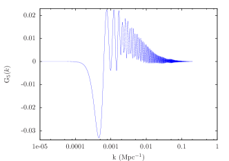
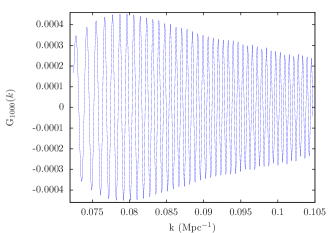
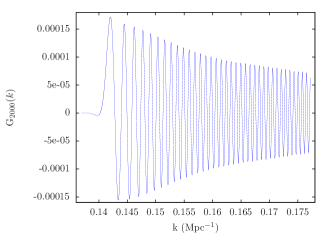
Then we plot Gl​(k)=∫0Ξ·0𝑑η​STs​(Ξ·,k)​jl​(x)subscriptπΊπ‘™π‘˜subscriptsuperscriptsubscriptπœ‚00differential-dπœ‚superscriptsubscriptπ‘†π‘‡π‘ πœ‚π‘˜subscript𝑗𝑙π‘₯G_{l}(k)=\int^{\eta_{0}}_{0}d\eta S_{T}^{s}(\eta,k)j_{l}(x) for l=5,1000,2000𝑙510002000l=5,1000,2000 in their main region (see Fig.(2,3,4)). One note that when l=5𝑙5l=5 Gl​(k)subscriptπΊπ‘™π‘˜G_{l}(k) is almost positive except for small kπ‘˜k where there exist a negative peak. One also note that for l=2000𝑙2000l=2000 the average period is longer than that for l=1000𝑙1000l=1000.

Refer to caption
Figure 2: Dependence of G5​(k)subscript𝐺5π‘˜G_{5}(k) on kπ‘˜k.
Refer to caption
Figure 3: Dependence of G1000​(k)subscript𝐺1000π‘˜G_{1000}(k) on kπ‘˜k.
Refer to caption
Figure 4: Dependence of G2000​(k)subscript𝐺2000π‘˜G_{2000}(k) on kπ‘˜k.

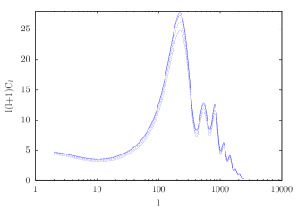
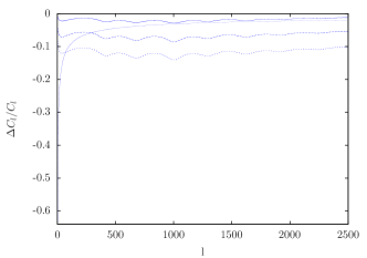
The CMB angular power spectra are plotted in Fig.(5) and the relative angular power spectra changes and the relative cosmic variance are plotted in Fig.(6). It is easy to note that the amplitude of angular power spectrum decreases when correlation is introduced. The greater is ΟƒπœŽ\sigma, the lower is the amplitude. From Fig.(6) it can be seen that the angular power spectrum decreases more significantly at the neighborhood of l=1000𝑙1000l=1000 than at smaller or larger l𝑙l. This is because of the phenomenon we mentioned in the last paragraph. Numerical calculation tells us that the contribution of F​(Ξ”)𝐹ΔF(\Delta) to Clsubscript𝐢𝑙C_{l} (Eq.(12)) concentrate at the neighbourhood of Ξ”=2​σΔ2𝜎\Delta=\sqrt{2\sigma} and kβ€²^β‹…k^β‰ˆ1β‹…^superscriptπ‘˜β€²^π‘˜1\hat{k^{{}^{\prime}}}\cdot\hat{k}\approx 1 in this case when ΟƒπœŽ\sigma is small (so Pl​(kβ€²^β‹…k^)β‰ˆ1subscript𝑃𝑙⋅^superscriptπ‘˜β€²^π‘˜1P_{l}(\hat{k^{{}^{\prime}}}\cdot\hat{k})\approx 1). Thus one can simply consider such a quantity C~l≑(4​π)2β€‹βˆ«0∞d​ln⁑k​Gl​(k)βˆ—Gl​(k+δ​k)subscript~𝐢𝑙superscript4πœ‹2superscriptsubscript0π‘‘π‘˜subscriptπΊπ‘™π‘˜subscriptπΊπ‘™π‘˜π›Ώπ‘˜\tilde{C}_{l}\equiv(4\pi)^{2}\int_{0}^{\infty}d\ln kG_{l}(k)*G_{l}(k+\delta k) (refer to Eq.(13)) and compare it with Cl=(4​π)2β€‹βˆ«0∞d​ln⁑k​(Gl​(k))2subscript𝐢𝑙superscript4πœ‹2superscriptsubscript0π‘‘π‘˜superscriptsubscriptπΊπ‘™π‘˜2C_{l}=(4\pi)^{2}\int_{0}^{\infty}d\ln k(G_{l}(k))^{2} to understand the above mentioned phenomenon, where δ​kπ›Ώπ‘˜\delta k is a small fixed value. From Fig.(2,3,4) one know that Gl​(k)subscriptπΊπ‘™π‘˜G_{l}(k) oscillate with kπ‘˜k, so one can further consider such a function,

f​(x)={0x<βˆ’1x+1βˆ’1≀x≀0βˆ’x+10≀x≀10x>1.𝑓π‘₯cases0π‘₯1π‘₯11π‘₯0π‘₯10π‘₯10π‘₯1f(x)=\left\{\begin{array}[]{cc}0&x<-1\\ x+1&-1\leq x\leq 0\\ -x+1&0\leq x\leq 1\\ 0&x>1.\end{array}\right.

The quantity D1β‰‘βˆ«f2​(x)​𝑑x=23subscript𝐷1superscript𝑓2π‘₯differential-dπ‘₯23D_{1}\equiv\int f^{2}(x)dx=\frac{2}{3}, while another quantity D2​(Ξ΄)β‰‘βˆ«f​(x)​f​(x+Ξ΄)​𝑑x=23βˆ’Ξ΄2​(1βˆ’Ξ΄2)subscript𝐷2𝛿𝑓π‘₯𝑓π‘₯𝛿differential-dπ‘₯23superscript𝛿21𝛿2D_{2}(\delta)\equiv\int f(x)f(x+\delta)dx=\frac{2}{3}-\delta^{2}(1-\frac{\delta}{2}) (here Ξ΄β‰ͺ1much-less-than𝛿1\delta\ll 1). One can see that D2<D1subscript𝐷2subscript𝐷1D_{2}<D_{1}. As the same reason, the angular power spectrum decrease when the primordial density fluctuation is correlated in Fourier space. At the same time, when 0<Ξ΄1<Ξ΄20subscript𝛿1subscript𝛿20<\delta_{1}<\delta_{2}, D2​(Ξ΄1)>D2​(Ξ΄2)subscript𝐷2subscript𝛿1subscript𝐷2subscript𝛿2D_{2}(\delta_{1})>D_{2}(\delta_{2}). Due to this, for a fix δ​kπ›Ώπ‘˜\delta k, C~lsubscript~𝐢𝑙\tilde{C}_{l} decrease less in the case that Gl​(k)subscriptπΊπ‘™π‘˜G_{l}(k) oscillates with a longer average period than the decrease in the case that Gl​(k)subscriptπΊπ‘™π‘˜G_{l}(k) oscillates with a shorter average period. Thus the angular power spectrum at large l𝑙l decrease less than that at about l∼1000similar-to𝑙1000l\sim 1000, since G1000​(k)subscript𝐺1000π‘˜G_{1000}(k) oscillates with a shorter average period compared with G2000​(k)subscript𝐺2000π‘˜G_{2000}(k). At last one note that when Gl​(k)subscriptπΊπ‘™π‘˜G_{l}(k) is always positive, the integrand Gl​(k)βˆ—Gl​(k+δ​k)subscriptπΊπ‘™π‘˜subscriptπΊπ‘™π‘˜π›Ώπ‘˜G_{l}(k)*G_{l}(k+\delta k) is also positive, while when Gl​(k)subscriptπΊπ‘™π‘˜G_{l}(k) is positive and negative alternate, the integrand Gl​(k)βˆ—Gl​(k+δ​k)subscriptπΊπ‘™π‘˜subscriptπΊπ‘™π‘˜π›Ώπ‘˜G_{l}(k)*G_{l}(k+\delta k) is not always positive. So when Gl​(k)subscriptπΊπ‘™π‘˜G_{l}(k) is always positive C~lsubscript~𝐢𝑙\tilde{C}_{l} tends to decrease less than the case that Gl​(k)subscriptπΊπ‘™π‘˜G_{l}(k) takes positive value and negative value alternately. This is the reason that the angular power spectrum decrease less at small l𝑙l than that at l=1000𝑙1000l=1000. These features can be used to constrain the correlation strength parameter ΟƒπœŽ\sigma from the real data.

Refer to caption
Figure 5: Unnormalized CMB angular power spectrum Clsubscript𝐢𝑙C_{l} as a function of l𝑙l. The solid line corresponds to the Gaussian random case, while the long dashed line, the short dashed line and the dotted line corresponds to Οƒ=10βˆ’10,5βˆ—10βˆ’10𝜎superscript10105superscript1010\sigma=10^{-10},5*10^{-10} and 10βˆ’9superscript10910^{-9} respectively.
Refer to caption
Figure 6: Dependence of Δ​ClClΞ”subscript𝐢𝑙subscript𝐢𝑙\frac{\Delta C_{l}}{C_{l}} on l𝑙l. Δ​ClΞ”subscript𝐢𝑙\Delta C_{l} is defined as the CMB angular power spectrum with correlation minus the one without correlation. The solid line, long dashed line and short dashed line correspond to Οƒ=10βˆ’10,5βˆ—10βˆ’10𝜎superscript10105superscript1010\sigma=10^{-10},5*10^{-10} and 10βˆ’9superscript10910^{-9} respectively. The dotted line is the cosmic variance of the angular power spectrum Δ​Cl/Cl=2/(2​l+1)Ξ”subscript𝐢𝑙subscript𝐢𝑙22𝑙1\Delta C_{l}/C_{l}=\sqrt{2/(2l+1)} in the uncorrelated case (here βˆ’2/(2​l+1)22𝑙1-\sqrt{2/(2l+1)} is plotted).

V Discussion

In this paper we only discussed a special type of the correlation of the primordial density fluctuation in the Fourier space. There exist other forms of correlation. From the point of experimental view, the correlation discussed in our paper is typical because the correlation between two modes is large only when they are almost the same. However, it is possible that the correlation in the Fourier space is scale dependent. Such possibilities can not be excluded. A better method is to divide these possible forms into several types, and then consider their effects on CMB. Besides CMB temperature, the effects on CMB polarization and large scale structure also need a further study.

Acknowledgements.
We would like to thank Dr Sun Weimin for improving the manuscript.

Appendix A Rotational Invariance

In this Appendix we shall give a proof for the statistically rotational invariance of Ts​(nβ†’β€²)​Ts​(nβ†’)superscript𝑇𝑠superscript→𝑛′superscript𝑇𝑠→𝑛T^{s}(\vec{n}^{{}^{\prime}})T^{s}(\vec{n}) and rotational invariance of F​(Ξ”β†’)𝐹→ΔF(\vec{\Delta}).

From Eq.(4), <Ts​(nβ†’β€²)​Ts​(nβ†’)>expectationsuperscript𝑇𝑠superscript→𝑛′superscript𝑇𝑠→𝑛<T^{s}(\vec{n}^{{}^{\prime}})T^{s}(\vec{n})> can be expressed as

<Ts​(nβ†’β€²)​Ts​(nβ†’)>expectationsuperscript𝑇𝑠superscript→𝑛′superscript𝑇𝑠→𝑛\displaystyle<T^{s}(\vec{n}^{{}^{\prime}})T^{s}(\vec{n})> (17)
=\displaystyle= ∫d3​kβ†’β€²β€‹βˆ«d3​kβ†’β€‹βˆ«0Ξ·0𝑑η′​STs​(Ξ·,kβ€²)​ei​x′​k^β€²β‹…n^β€²superscript𝑑3superscriptβ†’π‘˜β€²superscript𝑑3β†’π‘˜subscriptsuperscriptsubscriptπœ‚00differential-dsuperscriptπœ‚β€²superscriptsubscriptπ‘†π‘‡π‘ πœ‚superscriptπ‘˜β€²superscript𝑒⋅𝑖superscriptπ‘₯β€²superscript^π‘˜β€²superscript^𝑛′\displaystyle\int d^{3}\vec{k}^{{}^{\prime}}\int d^{3}\vec{k}\int^{\eta_{0}}_{0}d\eta^{{}^{\prime}}S_{T}^{s}(\eta,k^{{}^{\prime}})e^{ix^{{}^{\prime}}\hat{k}^{{}^{\prime}}\cdot\hat{n}^{{}^{\prime}}}
∫0Ξ·0𝑑η​STs​(Ξ·,k)​eβˆ’i​x​k^β‹…n^​<ξ​(kβ†’)β€‹ΞΎβˆ—β€‹(kβ†’β€²)>subscriptsuperscriptsubscriptπœ‚00differential-dπœ‚superscriptsubscriptπ‘†π‘‡π‘ πœ‚π‘˜superscript𝑒⋅𝑖π‘₯^π‘˜^𝑛expectationπœ‰β†’π‘˜superscriptπœ‰superscriptβ†’π‘˜β€²\displaystyle\int^{\eta_{0}}_{0}d\eta S_{T}^{s}(\eta,k)e^{-ix\hat{k}\cdot\hat{n}}<\xi(\vec{k})\xi^{*}(\vec{k}^{{}^{\prime}})>
=\displaystyle= ∫d3​kβ†’β€²β€‹βˆ«d3​kβ†’β€‹βˆ«0Ξ·0𝑑η′​STs​(Ξ·,kβ€²)​ei​x′​k^β€²β‹…n^β€²superscript𝑑3superscriptβ†’π‘˜β€²superscript𝑑3β†’π‘˜subscriptsuperscriptsubscriptπœ‚00differential-dsuperscriptπœ‚β€²superscriptsubscriptπ‘†π‘‡π‘ πœ‚superscriptπ‘˜β€²superscript𝑒⋅𝑖superscriptπ‘₯β€²superscript^π‘˜β€²superscript^𝑛′\displaystyle\int d^{3}\vec{k}^{{}^{\prime}}\int d^{3}\vec{k}\int^{\eta_{0}}_{0}d\eta^{{}^{\prime}}S_{T}^{s}(\eta,k^{{}^{\prime}})e^{ix^{{}^{\prime}}\hat{k}^{{}^{\prime}}\cdot\hat{n}^{{}^{\prime}}}
∫0Ξ·0𝑑η​STs​(Ξ·,k)​eβˆ’i​x​k^β‹…n^​f​(k,kβ€²,|kβ†’βˆ’kβ†’β€²|).subscriptsuperscriptsubscriptπœ‚00differential-dπœ‚superscriptsubscriptπ‘†π‘‡π‘ πœ‚π‘˜superscript𝑒⋅𝑖π‘₯^π‘˜^π‘›π‘“π‘˜superscriptπ‘˜β€²β†’π‘˜superscriptβ†’π‘˜β€²\displaystyle\int^{\eta_{0}}_{0}d\eta S_{T}^{s}(\eta,k)e^{-ix\hat{k}\cdot\hat{n}}f(k,k^{{}^{\prime}},|\vec{k}-\vec{k}^{{}^{\prime}}|).

Then the two point ensemble statistical average after rotation R𝑅R is

<Ts​(R​nβ†’β€²)​Ts​(R​nβ†’)>expectationsuperscript𝑇𝑠𝑅superscript→𝑛′superscript𝑇𝑠𝑅→𝑛\displaystyle<T^{s}(R\vec{n}^{{}^{\prime}})T^{s}(R\vec{n})> (18)
=\displaystyle= ∫d3​kβ†’β€²β€‹βˆ«d3​kβ†’β€‹βˆ«0Ξ·0𝑑η′​STs​(Ξ·,kβ€²)​ei​x′​k^β€²β‹…R​n^β€²superscript𝑑3superscriptβ†’π‘˜β€²superscript𝑑3β†’π‘˜subscriptsuperscriptsubscriptπœ‚00differential-dsuperscriptπœ‚β€²superscriptsubscriptπ‘†π‘‡π‘ πœ‚superscriptπ‘˜β€²superscript𝑒⋅𝑖superscriptπ‘₯β€²superscript^π‘˜β€²π‘…superscript^𝑛′\displaystyle\int d^{3}\vec{k}^{{}^{\prime}}\int d^{3}\vec{k}\int^{\eta_{0}}_{0}d\eta^{{}^{\prime}}S_{T}^{s}(\eta,k^{{}^{\prime}})e^{ix^{{}^{\prime}}\hat{k}^{{}^{\prime}}\cdot R\hat{n}^{{}^{\prime}}}
∫0Ξ·0𝑑η​STs​(Ξ·,k)​eβˆ’i​x​k^β‹…R​n^​f​(k,kβ€²,|kβ†’βˆ’kβ†’β€²|).subscriptsuperscriptsubscriptπœ‚00differential-dπœ‚superscriptsubscriptπ‘†π‘‡π‘ πœ‚π‘˜superscript𝑒⋅𝑖π‘₯^π‘˜π‘…^π‘›π‘“π‘˜superscriptπ‘˜β€²β†’π‘˜superscriptβ†’π‘˜β€²\displaystyle\int^{\eta_{0}}_{0}d\eta S_{T}^{s}(\eta,k)e^{-ix\hat{k}\cdot R\hat{n}}f(k,k^{{}^{\prime}},|\vec{k}-\vec{k}^{{}^{\prime}}|).

Replace the dummy variables kβ†’,kβ†’β€²\vec{k},\vec{k}{{}^{\prime}} by Rkβ†’,Rkβ†’β€²R\vec{k},R\vec{k}{{}^{\prime}} and note that d3​(R​kβ†’)=d3​kβ†’superscript𝑑3π‘…β†’π‘˜superscript𝑑3β†’π‘˜d^{3}(R\vec{k})=d^{3}\vec{k}, |R​kβ†’|=|kβ†’|π‘…β†’π‘˜β†’π‘˜|R\vec{k}|=|\vec{k}|, d3​(R​kβ†’β€²)=d3​kβ†’β€²superscript𝑑3𝑅superscriptβ†’π‘˜β€²superscript𝑑3superscriptβ†’π‘˜β€²d^{3}(R\vec{k}^{{}^{\prime}})=d^{3}\vec{k}^{{}^{\prime}}, |R​kβ†’β€²|=|kβ†’β€²|𝑅superscriptβ†’π‘˜β€²superscriptβ†’π‘˜β€²|R\vec{k}^{{}^{\prime}}|=|\vec{k}^{{}^{\prime}}| and |R​(kβ†’βˆ’kβ†’β€²)|=|kβ†’βˆ’kβ†’β€²|π‘…β†’π‘˜superscriptβ†’π‘˜β€²β†’π‘˜superscriptβ†’π‘˜β€²|R(\vec{k}-\vec{k}^{{}^{\prime}})|=|\vec{k}-\vec{k}^{{}^{\prime}}|, one obtains

<Ts​(R​nβ†’β€²)​Ts​(R​nβ†’)>expectationsuperscript𝑇𝑠𝑅superscript→𝑛′superscript𝑇𝑠𝑅→𝑛\displaystyle<T^{s}(R\vec{n}^{{}^{\prime}})T^{s}(R\vec{n})> (19)
=\displaystyle= ∫d3​kβ†’β€²β€‹βˆ«d3​kβ†’β€‹βˆ«0Ξ·0𝑑η′​STs​(Ξ·,kβ€²)​ei​x′​R​k^β€²β‹…R​n^β€²superscript𝑑3superscriptβ†’π‘˜β€²superscript𝑑3β†’π‘˜subscriptsuperscriptsubscriptπœ‚00differential-dsuperscriptπœ‚β€²superscriptsubscriptπ‘†π‘‡π‘ πœ‚superscriptπ‘˜β€²superscript𝑒⋅𝑖superscriptπ‘₯′𝑅superscript^π‘˜β€²π‘…superscript^𝑛′\displaystyle\int d^{3}\vec{k}^{{}^{\prime}}\int d^{3}\vec{k}\int^{\eta_{0}}_{0}d\eta^{{}^{\prime}}S_{T}^{s}(\eta,k^{{}^{\prime}})e^{ix^{{}^{\prime}}R\hat{k}^{{}^{\prime}}\cdot R\hat{n}^{{}^{\prime}}}
∫0Ξ·0𝑑η​STs​(Ξ·,k)​eβˆ’i​x​R​k^β‹…R​n^​f​(k,kβ€²,|kβ†’βˆ’kβ†’β€²|).subscriptsuperscriptsubscriptπœ‚00differential-dπœ‚superscriptsubscriptπ‘†π‘‡π‘ πœ‚π‘˜superscript𝑒⋅𝑖π‘₯𝑅^π‘˜π‘…^π‘›π‘“π‘˜superscriptπ‘˜β€²β†’π‘˜superscriptβ†’π‘˜β€²\displaystyle\int^{\eta_{0}}_{0}d\eta S_{T}^{s}(\eta,k)e^{-ixR\hat{k}\cdot R\hat{n}}f(k,k^{{}^{\prime}},|\vec{k}-\vec{k}^{{}^{\prime}}|).

Since R​k^β€²β‹…R​n^β€²=k^β€²β‹…n^′⋅𝑅superscript^π‘˜β€²π‘…superscript^𝑛′⋅superscript^π‘˜β€²superscript^𝑛′R\hat{k}^{{}^{\prime}}\cdot R\hat{n}^{{}^{\prime}}=\hat{k}^{{}^{\prime}}\cdot\hat{n}^{{}^{\prime}} and R​k^β‹…R​n^=k^β‹…n^⋅𝑅^π‘˜π‘…^𝑛⋅^π‘˜^𝑛R\hat{k}\cdot R\hat{n}=\hat{k}\cdot\hat{n}, one finally obtain

<Ts​(R​nβ†’β€²)​Ts​(R​nβ†’)>=<Ts​(nβ†’β€²)​Ts​(nβ†’)>.expectationsuperscript𝑇𝑠𝑅superscript→𝑛′superscript𝑇𝑠𝑅→𝑛expectationsuperscript𝑇𝑠superscript→𝑛′superscript𝑇𝑠→𝑛\displaystyle<T^{s}(R\vec{n}^{{}^{\prime}})T^{s}(R\vec{n})>=<T^{s}(\vec{n}^{{}^{\prime}})T^{s}(\vec{n})>. (20)

The same reasoning can be applied to F​(Ξ”β†’)𝐹→ΔF(\vec{\Delta}). From Eq.(10), one obtains

F​(R​Δ→)𝐹𝑅→Δ\displaystyle F(R\vec{\Delta}) =\displaystyle= (4​π)22​l+1β€‹βˆ‘m∫d3​k→′​d3​k→​Gl​(kβ€²)​Gl​(k)​Yl​m​(k^β€²)superscript4πœ‹22𝑙1subscriptπ‘šsuperscript𝑑3superscriptβ†’π‘˜β€²superscript𝑑3β†’π‘˜subscript𝐺𝑙superscriptπ‘˜β€²subscriptπΊπ‘™π‘˜subscriptπ‘Œπ‘™π‘šsuperscript^π‘˜β€²\displaystyle\dfrac{(4\pi)^{2}}{2l+1}\sum_{m}\int d^{3}\vec{k}^{{}^{\prime}}d^{3}\vec{k}G_{l}(k^{{}^{\prime}})G_{l}(k)Y_{lm}(\hat{k}^{{}^{\prime}}) (21)
Yl​mβˆ—β€‹(k^)​f​(k,kβ€²,|Ξ”β†’|)​δ3​(kβ†’βˆ’kβ†’β€²βˆ’R​Δ→).superscriptsubscriptπ‘Œπ‘™π‘š^π‘˜π‘“π‘˜superscriptπ‘˜β€²β†’Ξ”superscript𝛿3β†’π‘˜superscriptβ†’π‘˜β€²π‘…β†’Ξ”\displaystyle Y_{lm}^{*}(\hat{k})f(k,k^{{}^{\prime}},|\vec{\Delta}|)\delta^{3}(\vec{k}-\vec{k}^{{}^{\prime}}-R\vec{\Delta}).

Replace the dummy variables kβ†’,kβ†’β€²\vec{k},\vec{k}{{}^{\prime}} by Rkβ†’,Rkβ†’β€²R\vec{k},R\vec{k}{{}^{\prime}} as before and noted that d3​(R​kβ†’)=d3​kβ†’superscript𝑑3π‘…β†’π‘˜superscript𝑑3β†’π‘˜d^{3}(R\vec{k})=d^{3}\vec{k}, |R​kβ†’|=|kβ†’|π‘…β†’π‘˜β†’π‘˜|R\vec{k}|=|\vec{k}|, d3​(R​kβ†’β€²)=d3​kβ†’β€²superscript𝑑3𝑅superscriptβ†’π‘˜β€²superscript𝑑3superscriptβ†’π‘˜β€²d^{3}(R\vec{k}^{{}^{\prime}})=d^{3}\vec{k}^{{}^{\prime}}, |R​kβ†’β€²|=|kβ†’β€²|𝑅superscriptβ†’π‘˜β€²superscriptβ†’π‘˜β€²|R\vec{k}^{{}^{\prime}}|=|\vec{k}^{{}^{\prime}}|, |R​Δ→|=|Ξ”β†’|𝑅→Δ→Δ|R\vec{\Delta}|=|\vec{\Delta}|, Yl​m​(R​kβ†’β€²)=βˆ‘mβ€²Dm​mβ€²l​(R)​Yl​m​(kβ†’β€²)subscriptπ‘Œπ‘™π‘šπ‘…superscriptβ†’π‘˜β€²subscriptsuperscriptπ‘šβ€²subscriptsuperscriptπ·π‘™π‘šsuperscriptπ‘šβ€²π‘…subscriptπ‘Œπ‘™π‘šsuperscriptβ†’π‘˜β€²Y_{lm}(R\vec{k}^{{}^{\prime}})=\sum_{m^{{}^{\prime}}}D^{l}_{mm^{{}^{\prime}}}(R)Y_{lm}(\vec{k}^{{}^{\prime}}), Yl​mβˆ—β€‹(R​kβ†’)=βˆ‘mβ€²Dm​mβ€²lβ£βˆ—β€‹(R)​Yl​mβˆ—β€‹(kβ†’)subscriptsuperscriptπ‘Œπ‘™π‘šπ‘…β†’π‘˜subscriptsuperscriptπ‘šβ€²subscriptsuperscriptπ·π‘™π‘šsuperscriptπ‘šβ€²π‘…subscriptsuperscriptπ‘Œπ‘™π‘šβ†’π‘˜Y^{*}_{lm}(R\vec{k})=\sum_{m^{{}^{\prime}}}D^{l*}_{mm^{{}^{\prime}}}(R)Y^{*}_{lm}(\vec{k}) and Ξ΄3​[R​(kβ†’βˆ’kβ†’β€²βˆ’Ξ”β†’)]=Ξ΄3​(kβ†’βˆ’kβ†’β€²βˆ’Ξ”β†’)|R|=Ξ΄3​(kβ†’βˆ’kβ†’β€²βˆ’Ξ”β†’)superscript𝛿3delimited-[]π‘…β†’π‘˜superscriptβ†’π‘˜β€²β†’Ξ”superscript𝛿3β†’π‘˜superscriptβ†’π‘˜β€²β†’Ξ”π‘…superscript𝛿3β†’π‘˜superscriptβ†’π‘˜β€²β†’Ξ”\delta^{3}[R(\vec{k}-\vec{k}^{{}^{\prime}}-\vec{\Delta})]=\dfrac{\delta^{3}(\vec{k}-\vec{k}^{{}^{\prime}}-\vec{\Delta})}{|R|}=\delta^{3}(\vec{k}-\vec{k}^{{}^{\prime}}-\vec{\Delta}), one gets

F​(R​Δ→)=F​(Ξ”β†’).𝐹𝑅→Δ𝐹→Δ\displaystyle F(R\vec{\Delta})=F(\vec{\Delta}). (22)

.

References

  • Mukhanov and Chibisov (1981) V.Β F. Mukhanov and G.Β V. Chibisov, JETP Lett. 33, 532 (1981).
  • Starobinsky (1982) A.Β A. Starobinsky, Phys. Lett. B117, 175 (1982).
  • Guth and Pi (1982) A.Β H. Guth and S.Β Y. Pi, Phys. Rev. Lett. 49, 1110 (1982).
  • Hawking (1982) S.Β W. Hawking, Phys. Lett. B115, 295 (1982).
  • Smoot etΒ al. (1992) G.Β F. Smoot etΒ al., Astrophys. J. 396, L1 (1992).
  • Bennett etΒ al. (1996) C.Β L. Bennett etΒ al., Astrophys. J. 464, L1 (1996), eprint astro-ph/9601067.
  • Spergel etΒ al. (2007) D.Β N. Spergel etΒ al. (WMAP), Astrophys. J. Suppl. 170, 377 (2007), eprint astro-ph/0603449.
  • Hinshaw etΒ al. (2007) G.Β Hinshaw etΒ al. (WMAP), Astrophys. J. Suppl. 170, 288 (2007), eprint astro-ph/0603451.
  • Nayeri etΒ al. (2006) A.Β Nayeri, R.Β H. Brandenberger, and C.Β Vafa, Phys. Rev. Lett. 97, 021302 (2006), eprint hep-th/0511140.
  • Brandenberger etΒ al. (2007a) R.Β H. Brandenberger, A.Β Nayeri, S.Β P. Patil, and C.Β Vafa, Phys. Rev. Lett. 98, 231302 (2007a), eprint hep-th/0604126.
  • Brandenberger etΒ al. (2007b) R.Β H. Brandenberger, A.Β Nayeri, S.Β P. Patil, and C.Β Vafa, Int. J. Mod. Phys. A22, 3621 (2007b), eprint hep-th/0608121.
  • Brandenberger etΒ al. (2006) R.Β H. Brandenberger etΒ al., JCAP 0611, 009 (2006), eprint hep-th/0608186.
  • Carroll etΒ al. (2008) S.Β M. Carroll, C.-Y. Tseng, and M.Β B. Wise (2008), eprint 0811.1086.
  • Ackerman etΒ al. (2007) L.Β Ackerman, S.Β M. Carroll, and M.Β B. Wise, Phys. Rev. D75, 083502 (2007), eprint astro-ph/0701357.
  • Pullen and Kamionkowski (2007) A.Β R. Pullen and M.Β Kamionkowski, Phys. Rev. D76, 103529 (2007), eprint 0709.1144.
  • Groeneboom and Eriksen (2009) N.Β E. Groeneboom and H.Β K. Eriksen, Astrophys. J. 690, 1807 (2009), eprint 0807.2242.
  • Armendariz-Picon and Pekowsky (2008) C.Β Armendariz-Picon and L.Β Pekowsky (2008), eprint 0807.2687.
  • Perez etΒ al. (2006) A.Β Perez, H.Β Sahlmann, and D.Β Sudarsky, Class. Quant. Grav. 23, 2317 (2006), eprint gr-qc/0508100.
  • (19) S.Β Dodelson (2003), amsterdam, Netherlands: Academic Pr. (2003) 440 p.
  • Zaldarriaga and Seljak (1997) M.Β Zaldarriaga and U.Β Seljak, Phys. Rev. D55, 1830 (1997), eprint astro-ph/9609170.
  • Hu (2001) W.Β Hu, Phys. Rev. D64, 083005 (2001), eprint astro-ph/0105117.
  • Seljak and Zaldarriaga (1996) U.Β Seljak and M.Β Zaldarriaga, Astrophys. J. 469, 437 (1996), eprint astro-ph/9603033.