EUROPEAN ORGANIZATION FOR NUCLEAR RESEARCH

CERN-PH-EP/2007-XXX

27 August 2007

Measurement of $\alpha_{s}$ with Radiative Hadronic Events

The OPAL Collaboration

Abstract

Hadronic final states with a hard isolated photon are studied using data taken at centre-of-mass energies around the mass of the $\mathrm{Z}^{0}$ boson with the OPAL detector at LEP. The strong coupling $\alpha_{s}$ is extracted by comparing data and QCD predictions for event shape observables at average reduced centre-of-mass energies ranging from 24 GeV to 78 GeV, and the energy dependence of $\alpha_{s}$ is studied. Our results are consistent with the running of $\alpha_{s}$ as predicted by QCD and show that within the uncertainties of our analysis event shapes in hadronic $\mathrm{Z}^{0}$ decays with hard and isolated photon radiation can be described by QCD at reduced centre-of-mass energies. Combining all values from different event shape observables and energies gives $\alpha_{s}(M_{\mathrm{Z}})=0.1182\pm 0.0015(\mathrm{stat.})\pm 0.0101(\mathrm{syst.})$.

(to be submitted to Eur. Phys. J. C)

The OPAL Collaboration

G. Abbiendi², C. Ainsley⁵, P.F. Åkesson⁷, G. Alexander²¹, G. Anagnostou¹, K.J. Anderson⁸, S. Asai²², D. Axen²⁶, I. Bailey²⁵, E. Barberio^7,p, T. Barillari³¹, R.J. Barlow¹⁵, R.J. Batley⁵, P. Bechtle²⁴, T. Behnke²⁴, K.W. Bell¹⁹, P.J. Bell¹, G. Bella²¹, A. Bellerive⁶, G. Benelli⁴, S. Bethke³¹, O. Biebel³⁰, O. Boeriu⁹, P. Bock¹⁰, M. Boutemeur³⁰, S. Braibant², R.M. Brown¹⁹, H.J. Burckhart⁷, S. Campana⁴, P. Capiluppi², R.K. Carnegie⁶, A.A. Carter¹², J.R. Carter⁵, C.Y. Chang¹⁶, D.G. Charlton¹, C. Ciocca², A. Csilling²⁸, M. Cuffiani², S. Dado²⁰, M. Dallavalle², A. De Roeck⁷, E.A. De Wolf^7,s, K. Desch²⁴, B. Dienes²⁹, J. Dubbert³⁰, E. Duchovni²³, G. Duckeck³⁰, I.P. Duerdoth¹⁵, E. Etzion²¹, F. Fabbri², P. Ferrari⁷, F. Fiedler³⁰, I. Fleck⁹, M. Ford¹⁵, A. Frey⁷, P. Gagnon¹¹, J.W. Gary⁴, C. Geich-Gimbel³, G. Giacomelli², P. Giacomelli², M. Giunta⁴, J. Goldberg²⁰, E. Gross²³, J. Grunhaus²¹, M. Gruwé⁷, A. Gupta⁸, C. Hajdu²⁸, M. Hamann²⁴, G.G. Hanson⁴, A. Harel²⁰, M. Hauschild⁷, C.M. Hawkes¹, R. Hawkings⁷, G. Herten⁹, R.D. Heuer²⁴, J.C. Hill⁵, D. Horváth^28,c, P. Igo-Kemenes¹⁰, K. Ishii²², H. Jeremie¹⁷, P. Jovanovic¹, T.R. Junk^6,i, J. Kanzaki^22,u, D. Karlen²⁵, K. Kawagoe²², T. Kawamoto²², R.K. Keeler²⁵, R.G. Kellogg¹⁶, B.W. Kennedy¹⁹, S. Kluth³¹, T. Kobayashi²², M. Kobel^3,t, S. Komamiya²², T. Krämer²⁴, A. Krasznahorkay Jr.^29,e, P. Krieger^6,l, J. von Krogh¹⁰, T. Kuhl²⁴, M. Kupper²³, G.D. Lafferty¹⁵, H. Landsman²⁰, D. Lanske¹³, D. Lellouch²³, J. Letts^o, L. Levinson²³, J. Lillich⁹, S.L. Lloyd¹², F.K. Loebinger¹⁵, J. Lu^26,b, A. Ludwig^3,t, J. Ludwig⁹, W. Mader^3,t, S. Marcellini², A.J. Martin¹², T. Mashimo²², P. Mättig^m, J. McKenna²⁶, R.A. McPherson²⁵, F. Meijers⁷, W. Menges²⁴, F.S. Merritt⁸, H. Mes^6,a, N. Meyer²⁴, A. Michelini², S. Mihara²², G. Mikenberg²³, D.J. Miller¹⁴, W. Mohr⁹, T. Mori²², A. Mutter⁹, K. Nagai¹², I. Nakamura^22,v, H. Nanjo²², H.A. Neal³², S.W. O’Neale^1,∗, A. Oh⁷, M.J. Oreglia⁸, S. Orito^22,∗, C. Pahl³¹, G. Pásztor^4,g, J.R. Pater¹⁵, J.E. Pilcher⁸, J. Pinfold²⁷, D.E. Plane⁷, O. Pooth¹³, M. Przybycień^7,n, A. Quadt³¹, K. Rabbertz^7,r, C. Rembser⁷, P. Renkel²³, J.M. Roney²⁵, A.M. Rossi², Y. Rozen²⁰, K. Runge⁹, K. Sachs⁶, T. Saeki²², E.K.G. Sarkisyan^7,j, A.D. Schaile³⁰, O. Schaile³⁰, P. Scharff-Hansen⁷, J. Schieck³¹, T. Schörner-Sadenius^7,z, M. Schröder⁷, M. Schumacher³, R. Seuster^13,f, T.G. Shears^7,h, B.C. Shen^4,∗, P. Sherwood¹⁴, A. Skuja¹⁶, A.M. Smith⁷, R. Sobie²⁵, S. Söldner-Rembold¹⁵, F. Spano^8,x, A. Stahl¹³, D. Strom¹⁸, R. Ströhmer³⁰, S. Tarem²⁰, M. Tasevsky^7,d, R. Teuscher⁸, M.A. Thomson⁵, E. Torrence¹⁸, D. Toya²², I. Trigger^7,w, Z. Trócsányi^29,e, E. Tsur²¹, M.F. Turner-Watson¹, I. Ueda²², B. Ujvári^29,e, C.F. Vollmer³⁰, P. Vannerem⁹, R. Vértesi^29,e, M. Verzocchi¹⁶, H. Voss^7,q, J. Vossebeld^7,h, C.P. Ward⁵, D.R. Ward⁵, P.M. Watkins¹, A.T. Watson¹, N.K. Watson¹, P.S. Wells⁷, T. Wengler⁷, N. Wermes³, G.W. Wilson^15,k, J.A. Wilson¹, G. Wolf²³, T.R. Wyatt¹⁵, S. Yamashita²², D. Zer-Zion⁴, L. Zivkovic²⁰

¹School of Physics and Astronomy, University of Birmingham, Birmingham B15 2TT, UK
²Dipartimento di Fisica dell’ Università di Bologna and INFN, I-40126 Bologna, Italy
³Physikalisches Institut, Universität Bonn, D-53115 Bonn, Germany
⁴Department of Physics, University of California, Riverside CA 92521, USA
⁵Cavendish Laboratory, Cambridge CB3 0HE, UK
⁶Ottawa-Carleton Institute for Physics, Department of Physics, Carleton University, Ottawa, Ontario K1S 5B6, Canada
⁷CERN, European Organisation for Nuclear Research, CH-1211 Geneva 23, Switzerland
⁸Enrico Fermi Institute and Department of Physics, University of Chicago, Chicago IL 60637, USA
⁹Fakultät für Physik, Albert-Ludwigs-Universität Freiburg, D-79104 Freiburg, Germany
¹⁰Physikalisches Institut, Universität Heidelberg, D-69120 Heidelberg, Germany
¹¹Indiana University, Department of Physics, Bloomington IN 47405, USA
¹²Queen Mary and Westfield College, University of London, London E1 4NS, UK
¹³Technische Hochschule Aachen, III Physikalisches Institut, Sommerfeldstrasse 26-28, D-52056 Aachen, Germany
¹⁴University College London, London WC1E 6BT, UK
¹⁵School of Physics and Astronomy, Schuster Laboratory, The University of Manchester M13 9PL, UK
¹⁶Department of Physics, University of Maryland, College Park, MD 20742, USA
¹⁷Laboratoire de Physique Nucléaire, Université de Montréal, Montréal, Québec H3C 3J7, Canada
¹⁸University of Oregon, Department of Physics, Eugene OR 97403, USA
¹⁹Rutherford Appleton Laboratory, Chilton, Didcot, Oxfordshire OX11 0QX, UK
²⁰Department of Physics, Technion-Israel Institute of Technology, Haifa 32000, Israel
²¹Department of Physics and Astronomy, Tel Aviv University, Tel Aviv 69978, Israel
²²International Centre for Elementary Particle Physics and Department of Physics, University of Tokyo, Tokyo 113-0033, and Kobe University, Kobe 657-8501, Japan
²³Particle Physics Department, Weizmann Institute of Science, Rehovot 76100, Israel
²⁴Universität Hamburg/DESY, Institut für Experimentalphysik, Notkestrasse 85, D-22607 Hamburg, Germany
²⁵University of Victoria, Department of Physics, P O Box 3055, Victoria BC V8W 3P6, Canada
²⁶University of British Columbia, Department of Physics, Vancouver BC V6T 1Z1, Canada
²⁷University of Alberta, Department of Physics, Edmonton AB T6G 2J1, Canada
²⁸Research Institute for Particle and Nuclear Physics, H-1525 Budapest, P O Box 49, Hungary
²⁹Institute of Nuclear Research, H-4001 Debrecen, P O Box 51, Hungary
³⁰Ludwig-Maximilians-Universität München, Sektion Physik, Am Coulombwall 1, D-85748 Garching, Germany
³¹Max-Planck-Institut für Physik, Föhringer Ring 6, D-80805 München, Germany
³²Yale University, Department of Physics, New Haven, CT 06520, USA

^a and at TRIUMF, Vancouver, Canada V6T 2A3
^b now at University of Alberta
^c and Institute of Nuclear Research, Debrecen, Hungary
^d now at Institute of Physics, Academy of Sciences of the Czech Republic 18221 Prague, Czech Republic
^e and Department of Experimental Physics, University of Debrecen, Hungary
^f and MPI München
^g and Research Institute for Particle and Nuclear Physics, Budapest, Hungary
^h now at University of Liverpool, Dept of Physics, Liverpool L69 3BX, U.K.
ⁱ now at Dept. Physics, University of Illinois at Urbana-Champaign, U.S.A.
^j and The University of Manchester, M13 9PL, United Kingdom
^k now at University of Kansas, Dept of Physics and Astronomy, Lawrence, KS 66045, U.S.A.
^l now at University of Toronto, Dept of Physics, Toronto, Canada
^m current address Bergische Universität, Wuppertal, Germany
ⁿ now at University of Mining and Metallurgy, Cracow, Poland
^o now at University of California, San Diego, U.S.A.
^p now at The University of Melbourne, Victoria, Australia
^q now at IPHE Université de Lausanne, CH-1015 Lausanne, Switzerland
^r now at IEKP Universität Karlsruhe, Germany
^s now at University of Antwerpen, Physics Department,B-2610 Antwerpen, Belgium; supported by Interuniversity Attraction Poles Programme – Belgian Science Policy
^t now at Technische Universität, Dresden, Germany
^u and High Energy Accelerator Research Organisation (KEK), Tsukuba, Ibaraki, Japan
^v now at University of Pennsylvania, Philadelphia, Pennsylvania, USA
^w now at TRIUMF, Vancouver, Canada
^x now at Columbia University
^y now at CERN
^z now at DESY
^∗ Deceased

1 Introduction

In the theory of strong interactions, Quantum Chromodynamics (QCD) [1, 2, 3], the strong coupling constant $\alpha_{s}$ is predicted to decrease for high energy or short distance reactions: a phenomenon known as asymptotic freedom. The values of $\alpha_{s}$ at different energy scales have been measured in $\mathrm{e}^{+}\mathrm{e}^{-}$ reactions with different centre-of-mass (cms) energies ranging from 35 to 209 GeV and confirm the prediction [4, 5, 6, 7, 8, 9, 10, 11].

Assuming that photons emitted before or immediately after the $\mathrm{Z}^{0}$ production do not interfere with hard QCD processes, a measurement of $\alpha_{s}$ at the reduced cms energies, $\sqrt{s^{\prime}}$, of the hadronic system is possible by using radiative multi-hadronic events, i.e. $\mathrm{e}^{+}\mathrm{e}^{-}\rightarrow\mathrm{q\bar{q}}\gamma$ events.

Most photons emitted from the incoming particles before the $\mathrm{Z}^{0}$ production (initial state radiation, ISR) escape along the beam pipe of the experiment. Measurements of cross-sections for hadron production with ISR have been presented by the KLOE and BaBar collaborations [12, 13, 14, 15]. In $\mathrm{e}^{+}\mathrm{e}^{-}$ annihilation to hadrons on the $\mathrm{Z}^{0}$ peak isolated high energy photons observed in the detector are mostly emitted by quarks produced in hadronic $\mathrm{Z}^{0}$ decays (final state radiation, FSR), because on the $\mathrm{Z}^{0}$ peak ISR effects are supressed. Measurements of $\alpha_{s}$ in hadronic events with observed photons have been performed by the L3 and DELPHI Collaborations [16, 17]. The DELPHI collaboration has also measured the mean charged particle multiplicity $\langle n_{\mathrm{ch}}\rangle(s^{\prime})$ using FSR in [18].

When an energetic and isolated photon is emitted in the parton shower the invariant mass of the recoiling parton system is taken to set the energy scale for hard QCD processes such as gluon radiation. In parton shower models [19, 20, 21] the invariant mass of an intermediate parton or the transverse momentum of a parton branching are used as ordering parameters for the parton shower development. In this picture an energetic and isolated photon must be produced at an early stage of the shower evolution and therefore can be used to deduce the scale for subsequent QCD processes. The validity of this method will be studied below using parton shower Monte Carlo programs.

Here we report on a measurement of $\alpha_{s}$ from event shape observables determined from the hadronic system in events with observed energetic and isolated photons in the OPAL experiment.

2 Analysis method

The reduced cms energy, $\sqrt{s^{\prime}}$, is defined by $2E_{\mathrm{beam}}\sqrt{1-E_{\gamma}/E_{\mathrm{beam}}}$, where $E_{\gamma}$ is the photon energy and $E_{\mathrm{beam}}$ is the beam energy. The flavour mixture of hadronic events in this analysis is changed compared to non-radiative $\mathrm{Z}^{0}$ decay events. The fraction of up-type quarks is larger due to their larger electric charge. However, since the strong interaction is blind to quark flavour in the Standard Model, as e.g. demonstrated in [22], the difference is not taken into account.

The determination of $\alpha_{s}$ is based on measurements of event shape observables, which are calculated from all particles with momenta $p_{i}$ in an event:

Thrust $T$.

The thrust $T$ is defined by the expression

$$T=\max_{\vec{\hat{n}}}\left(\frac{\sum_{i}|\vec{p}_{i}\cdot\vec{\hat{n}}|}{\sum_{i}|\vec{p}_{i}|}\right)\;\;\;.$$ (1)

The thrust axis $\vec{\hat{n}}_{T}$ is the direction $\vec{\hat{n}}$ which maximises the expression in parentheses. A plane through the origin and perpendicular to $\vec{\hat{n}}_{T}$ divides the event into two hemispheres $H_{1}$ and $H_{2}$.

Heavy Jet Mass $M_{H}$.

The hemisphere invariant masses are calculated using the particles in the two hemispheres $H_{1}$ and $H_{2}$. We define $M_{H}$ as the heavier mass, divided by $\sqrt{s}$ .

Jet Broadening variables $B_{T}$ and $B_{W}$.

These are defined by computing the quantity

$$B_{k}=\left(\frac{\sum_{i\in H_{k}}|\vec{p}_{i}\times\vec{\hat{n}}_{T}|}{2\sum_{i}|\vec{p}_{i}|}\right)$$ (2)

for each of the two event hemispheres, $H_{k}$, defined above. The two observables are defined by

$$B_{T}=B_{1}+B_{2}\;\;\;\mathrm{and}\;\;\;B_{W}=\max(B_{1},B_{2})\;\;\;$$ (3)

where $B_{T}$ is the total and $B_{W}$ is the wide jet broadening.

C-parameter $C$.

The linear momentum tensor $\Theta^{\alpha\beta}$ is defined by

$$\Theta^{\alpha\beta}=\frac{\sum_{i}\vec{p}_{i}^{\alpha}\vec{p}_{i}^{\beta}/|\vec{p}_{i}|}{\sum_{j}|\vec{p}_{j}|}\ ,\ \alpha,\beta=1,2,3.$$ (4)

The three eigenvalues $\lambda_{j}$ of this tensor define $C$ with

$$C=3(\lambda_{1}\lambda_{2}+\lambda_{2}\lambda_{3}+\lambda_{3}\lambda_{1}).$$ (5)

Transition value $y_{23}^{D}$.

This observable is given by the value of $y_{cut}$ in the Durham algorithm where the number of jets in an event changes from two to three.

In order to verify that using hadronic $\mathrm{Z}^{0}$ decays with hard and isolated final state radiation allows one to extract $\alpha_{s}$ at a reduced scale $\sqrt{s^{\prime}}$ we employ simulated events. We use the Monte Carlo simulation programs JETSET version 7.4 [19], HERWIG version 5.9 [20] and ARIADNE version 4.08 [21], which have different implementations of the parton shower algorithms including simulation of FSR. One sample contains hadronic $\mathrm{Z}^{0}$ decays with FSR and ISR (375 k events) while the other samples are generated at lower cms energies without ISR (500 k events each).

We consider the generated events after the parton shower has stopped (parton-level) and calculate event shape observables using the remaining partons. The effective cms energy $\sqrt{s^{\prime}}$ is calculated from the parton four-momenta excluding any final state photons and the events are boosted into the cms system of the partons. The samples are binned according to the energy $E_{\mathrm{FSR}}$ of any FSR in intervals of 5 GeV width for $E_{\mathrm{FSR}}>10$ GeV.

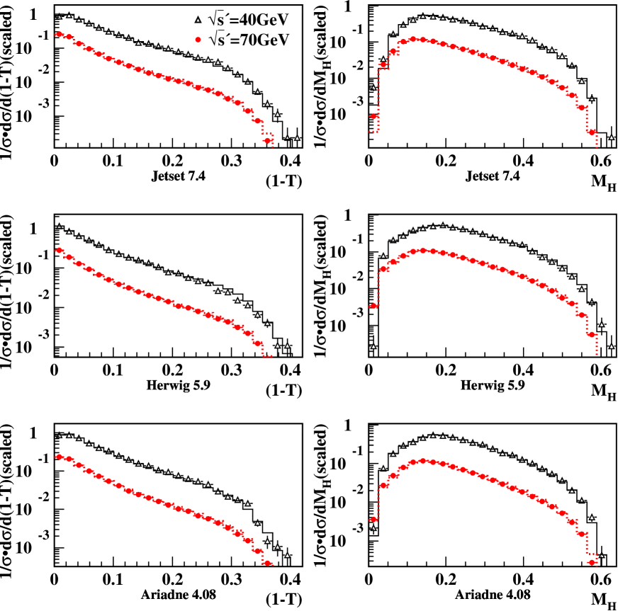
We observe good agreement between the corresponding distributions obtained from the $\mathrm{Z}^{0}$ sample with FSR and the lower energy samples. For example, Figure 1 shows distributions of the event shape observables $1-T$ and $M_{H}$ for two samples with $\sqrt{s^{\prime}}=40$ and 70 GeV. We conclude that within the approximations made in the parton shower algorithms, hadronic $\mathrm{Z}^{0}$ decays with hard and isolated final state radiation can be used to extract measurements of $\alpha_{s}$ at reduced scales $\sqrt{s^{\prime}}$.

3 The OPAL Detector and Event Simulation

The OPAL detector operated at the LEP $\mathrm{e}^{+}\mathrm{e}^{-}$ collider at CERN from 1989 to 2000. A detailed description of the detector can be found in [23]. We describe briefly the important parts of the detector for this study. In the OPAL coordinate system, the $x$ axis was horizontal and pointed approximately towards the centre of LEP, the $y$ axis was normal to the $z$-$x$ plane , and the $z$ axis was in the $\mathrm{e}^{-}$ beam direction. The polar angle, $\theta$, was measured from the $z$ axis, and the azimuthal angle, $\phi$, from the $x$ axis about the $z$ axis.

The central detector measured the momentum of charged particles and consisted of a system of cylindrical drift chambers which lay within an axial magnetic field of 0.435 T. The momenta $p_{xy}$ of tracks in the $x$-$y$ plane were measured with a precision of $\sigma_{p}/p_{xy}=0.02\%\oplus 0.0015\cdot p_{xy}[\mathrm{GeV}/c]$ [24].

The electromagnetic calorimeters completely covered the azimuthal range for polar angles satisfying $|\cos{\theta}|<0.98$. The barrel electromagnetic calorimeter covered the polar angle range $|\cos{\theta}|<0.82$, and consisted of a barrel of 9440 lead glass blocks oriented so that they nearly pointed to the interaction region. The two endcaps were each made of 1132 lead glass blocks, aligned along the $z$-axis. Each lead glass block in the barrel electromagnetic calorimeter was 10$\times$10 cm² in cross section, which corresponds to an angular region of approximately $40\times 40$ mrad². The intrinsic energy resolution was $\sigma_{E}/E=0.2\%\oplus 6.3\%/\sqrt{E[\mathrm{GeV}]}$ [23].

Most electromagnetic showers were initiated before the lead glass mainly because of the coil and pressure vessel in front of the calorimeter. An electromagnetic presampler made of limited streamer tubes measured the shower position. The barrel presampler covered the polar angle range $|\cos{\theta}|<0.81$ and its angular resolution for photons was approximately 2 mrad.

JETSET version 7.4 was used to simulate $\mathrm{e}^{+}\mathrm{e}^{-}\rightarrow\mathrm{q\bar{q}}$ events, with HERWIG version 5.9 and ARIADNE version 4.08 used as alternatives. Parameters controlling the hadronisation of quarks and gluons were tuned to OPAL LEP 1 data as described in [25, 26]. We used HERWIG version 5.8 [20], PHOJET version 1.05c [27, 28] and VERMASEREN version 1.01 [29] for two-photon interactions and KORALZ version 4.02 [30] for $\mathrm{e}^{+}\mathrm{e}^{-}\rightarrow\tau^{+}\tau^{-}$ events. Generated events were processed through a full simulation of the OPAL detector [31] and the same event analysis chain was applied to the simulated events as to the data. 4,000,000 fully simulated events were generated by JETSET, 200,000 events, 1,000,000 events and 55,000 events were generated by HERWIG, PHOJET and VERMASEREN while 800,000 events were generated by KORALZ.

4 Event Selection

4.1 Hadronic Event Selection

This study is based on a sample of 3 million hadronic $\mathrm{Z}^{0}$ decays selected as described in [32] from the data accumulated between 1992 and 1995 at cms energy of 91.2 GeV. We required that the central detector and the electromagnetic calorimeter were fully operational.

For this study, we apply stringent cuts on tracks and clusters and further cuts on hadronic events. The clusters in the electromagnetic calorimeter are required to have a minimum energy of 100 MeV in the barrel and 250 MeV in the endcap. Tracks are required to have transverse momentum $p_{T}\geq 150~{}\mathrm{MeV}/c$ with respect to the beam axis, at least 40 reconstructed points in the jet chamber, at the point of closest approach a distance between the track and the nominal vertex $d_{0}<2$ cm in the $r$-$\phi$ plane and $z_{0}<25$ cm in the $z$ direction. We require at least five such tracks to reduce background from $\mathrm{e}^{+}\mathrm{e}^{-}\rightarrow\tau^{+}\tau^{-}$ and $\gamma\gamma\rightarrow\mathrm{q\bar{q}}$ events. The polar angle of the thrust axis is required to satisfy $|\cos{\theta_{T}}|<0.9$, to ensure that events are well contained in the OPAL detector. After these cuts, a data sample of $2.4\times 10^{6}$ events remains.

4.2 Isolated Photon Selection

4.2.1 Isolation Cuts

Isolated photons are selected in these hadronic events as follows. Electromagnetic clusters with an energy $E_{\mathrm{EC}}>10$ GeV are chosen in order to suppress background from soft photons coming from the decay of mesons. Accordingly, our signal event is defined as an $\mathrm{e}^{+}\mathrm{e}^{-}\rightarrow\mathrm{q\bar{q}}$ event with an ISR or FSR photon with energy greater than 10 GeV. We use electromagnetic clusters in the polar angle region $|\cos{\theta_{\mathrm{EC}}}|<0.72$ corresponding to the barrel of the detector, where there is the least material in front of the lead glass, see Figure 2 a). Also, the non-pointing geometry of the endcap electromagnetic calorimeter complicates the cluster shape fitting explained below. The number of clusters in the data which satisfy $E_{\mathrm{EC}}>10$ GeV and $|\cos{\theta_{\mathrm{EC}}}|<0.72$ is 1,797,532. According to the Monte Carlo simulation, 99.3% of these selected clusters come from non-radiative multi-hadronic events.

The candidate clusters are required to be isolated from any jets, and from other clusters and tracks:

• The angle with respect to the axis of any jet, $\alpha_{\mathrm{iso}}$, is required to be larger than $25^{\circ}$, see Figure 2 b). The jets are reconstructed from tracks and electromagnetic clusters, excluding the candidate cluster, using the Durham algorithm[33] with $y_{\mathrm{cut}}=0.005$.

• The sum of the momenta $P_{\mathrm{iso}}$ of tracks falling on the calorimeter surface inside a 0.2 radian cone around the photon candidate is required to be smaller than 0.5 $\mathrm{GeV}/c$ (Figure 2 c)). The total energy deposition in the electromagnetic calorimeter within a cone of 0.2 radian around the photon candidate, $E_{\mathrm{iso}}$, is also required to be less than 0.5 GeV (Figure 2 d)).

After the isolation cuts, 11,265 clusters are retained. The fraction of clusters from non-radiative multi-hadronic events is reduced to 52.8%. The background from $\tau^{+}\tau^{-}$ events (two-photon events) is 0.6% (0.01%) [34].

4.2.2 Likelihood Photon Selection

Isolated photon candidates are selected by using a likelihood ratio method [35] with four input variables. The first two variables are $|\cos{\theta_{\mathrm{EC}}}|$ and $\alpha_{\mathrm{iso}}$, defined above. Two more variables, the cluster shape fit variable $S$ and the distance $\Delta$ between the electromagnetic calorimeter cluster and the associated presampler cluster, defined as follows, reduce the background from clusters arising from the decays of neutral hadrons.

The cluster shape fit variable, $S$, is defined by

$$S=\frac{1}{N_{\mathrm{block}}}\sum_{i}{\frac{(E_{\mathrm{meas},i}-E_{\mathrm{exp},i})^{2}}{\sigma_{\mathrm{meas},i}^{2}}}$$ (6)

where $N_{\mathrm{block}}$ is the number of lead glass blocks included in the electromagnetic cluster, $E_{\mathrm{meas},i}$ is the measured energy deposit in the $i$th block, $E_{\mathrm{exp},i}$ is the expected energy deposit in the $i$th block, assuming that the energy is deposited by a single photon, and $\sigma_{\mathrm{meas},i}$ is the uncertainty in the energy measured by $i$th electromagnetic calorimeter block. $E_{\mathrm{exp},i}$ is a function of position and energy of the incident photon based on the simulation of the OPAL detector with single photons. The value of $S$ is determined by minimizing Equation (6) under variation of the position and energy of the cluster. For a cluster to be considered further in the likelihood, preselection cuts are applied: we require the number of blocks to be at least two and the value of $S$ after the fit to be smaller than 10. The quality of the cluster shape fits depends on the assumed resolution $\sigma_{\mathrm{meas},i}$; this will be studied as a systematic uncertainty.

The variable $\Delta$ measures the distance between the electromagnetic calorimeter cluster and the associated presampler cluster, $\Delta=\max(|\Delta\phi|,|\Delta\theta|)$, with $\Delta\phi$ and $\Delta\theta$ the angular separations between the clusters.

The distributions of $S$ and $\Delta$ are shown in Figures 2 e) and f). The Monte Carlo distributions in these figures are normalized according to the luminosity obtained from small angle Bhabha events.

A disagreement between data and Monte Carlo is seen for $S$ and $\alpha_{\mathrm{iso}}$. The level of agreement between data and Monte Carlo for the $S$ distribution is studied with photons in radiative muon pair events and $\pi^{0}$s produced in tau pair events. It is confirmed that the Monte Carlo adequately reproduces the $S$ distributions [34]. The disagreement between data and Monte Carlo for distributions of $S$ and $\alpha_{\mathrm{iso}}$ stems from the failure of the Monte Carlo generators to correctly predict the rate of isolated neutral hadrons, as explained in Section 4.4. In this analysis, the rate of isolated neutral hadrons used in the background subtraction is estimated from data by methods described in Section 4.4.

The likelihood calculation is performed with reference histograms made for seven subsamples, chosen according to the cluster energy. The cut on the likelihood value is chosen so as to retain 80% of the signal events. The likelihood distributions for data and Monte Carlo are shown in Figure 3. It can be seen that the likelihood distributions for signal and background events are well separated for each region of electromagnetic cluster energy. The correlations between variables are taken into account using the algorithm described in [36]. Electromagnetic clusters which pass the likelihood selection are regarded as photon candidates. If more than one candidate is found in the same event the one with the highest energy is chosen.

4.3 Final Data Sample

Hadronic events with hard isolated photon candidates are divided into seven subsamples according to the photon energy for further analysis. Table 1 shows the mean values of $\sqrt{s^{\prime}}$, the number of data events and the number of background events for each subsample.

4.4 Background Estimation

According to the Monte Carlo simulation, the contamination from $\tau$ pair events is between 0.5 and 1.0%. The impact of this small number of events is further reduced because the value of event shape observables for $\tau$ pair events are concentrated in the lowest bin of the distributions, outside the fitting range, so their effect on the $\alpha_{s}$ fits is negligible. The contribution of two photon processes is less than 0.01% in all subsamples and is ignored.

As mentioned in [37], the JETSET Monte Carlo fails to reproduce the observed rate of isolated electromagnetic clusters, both for isolated photons and isolated $\pi^{0}$’s. Isolated neutral hadrons are the dominant source of background for this analysis, and their rate has been estimated from data using the following two methods.

Firstly, with the likelihood ratio method the observed likelihood distributions in the data in bins of photon energy were fitted with a linear combination of the Monte Carlo distributions for signal and background events which pass the isolation cuts and likelihood preselection requirements. The overall normalisation of the Monte Carlo distribution is fixed to the number of data events. The fit uses a binned maximum likelihood method with only the fraction of background events as a free parameter. Figure 3 shows the fit results. The values of $\chi^{2}/\mathrm{d.o.f.}$ are between 1.2 and 3.4 for 18 degrees of freedom.

Secondly, with the isolated tracks method the fraction of background from isolated neutral hadrons was estimated from the rates of isolated charged hadrons. We select from the data tracks which satisfy the same isolation criteria as the photon candidates. The composition of these isolated charged hadrons obtained from JETSET is used to infer the rates of charged pions, kaons and protons. When isospin symmetry is assumed, the rates of neutral pions, neutral kaons and neutrons can be estimated from the rates of charged pions, charged kaons and protons, respectively:

$$R_{\pi^{0}}=\frac{1}{2}R_{\pi^{\pm}}\hskip 28.45274ptR_{\mathrm{K}^{0}_{\mathrm{L}}}=\frac{1}{2}R_{\mathrm{K}^{\pm}}\hskip 28.45274ptR_{\mathrm{n}}=R_{\mathrm{p}}\ ,$$ (7)

where $R_{\mathrm{X}}$ is the production rate of particle X. According to JETSET tuned with OPAL data, the rate of isospin symmetry violation is 10% for pions and 5% for kaons and protons. This is assigned as a systematic uncertainty for the isolated tracks method and combined with the statistical uncertainty.

The neutral hadron background fractions estimated by these two methods are shown in Table 1. The statistical errors from the number of data and Monte Carlo events from fitting the likelihood distributions are shown. The results from the two methods are within at most three standard deviations of these errors, except in the $E_{\gamma}$ bin $35-40$ GeV.

The standard analysis will use the likelihood ratio method. Any differences in the resulting values of $\alpha_{s}$ obtained by using the two background estimate methods will be treated as a systematic uncertainty.

5 Measurement of Event Shape Distributions

In this analysis event shape observables as defined above in section 2 are calculated from tracks and electromagnetic clusters excluding the isolated photon candidate. The contributions of electromagnetic clusters originating from charged particles are removed by the method described in [38].

We evaluate the observables in the cms frame of the hadronic system. The Lorentz boost is determined from the energy and angle of the photon candidate. When the four-momentum of particles in the hadronic system is calculated, electromagnetic clusters are treated as photons with zero mass while tracks of charged particles are treated as hadrons with the charged pion mass.

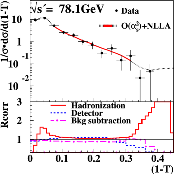
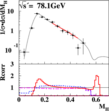
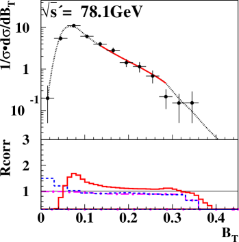
Distributions of the event shape observables ($1-T$) and $M_{H}$ are shown for two cms energies in Figure 4. The remaining background is removed by subtracting the scaled Monte Carlo predictions for non-radiative hadronic events and for $\tau$ pair events using the background estimates listed in Table 1. The effects of the experimental resolution and acceptance are unfolded using Monte Carlo samples with full detector simulation (detector correction). The unfolding is performed bin-by-bin with correction factors $r_{i}^{Det}=h_{i}/d_{i}$, where $h_{i}$ represents the value in the $i$th bin of the event shape distribution of stable hadrons in the Monte Carlo simulation, where “hadrons” are defined as particles with a mean proper lifetime longer than $3\cdot 10^{-10}$s. $d_{i}$ represents the value in the $i$th bin of the event shape distribution calculated with clusters and tracks obtained from Monte Carlo samples with detector simulation after the complete event selection has been applied. We refer to the distributions after applying these corrections as data corrected to the hadron level.

The distributions of the event shape observables $1-T$ and $M_{H}$ for data corrected to the hadron level and corresponding Monte Carlo predictions are shown in Figure 5. The Monte Carlo samples are generated with cms energies set to the mean value of $\sqrt{s^{\prime}}$ in each subsample. In the production of the Monte Carlo samples ISR and FSR is switched off and on, respectively. The predictions from the event generators are consistent with the data for all $\sqrt{s^{\prime}}$ bins. There is similar agreement between data and event generator predictions for the other observables.

6 Measurement of $\alpha_{s}$

The measurement of $\alpha_{s}$ is performed by fitting perturbative QCD predictions to the event shape distributions corrected to the hadron level for ($1-T$), $M_{H}$ [39], $B_{T}$, $B_{W}$ [41, 40], $C$ [42, 43] and $y_{23}^{D}$ [33, 44, 45]. The $\mathcal{O}(\alpha_{s}^{2})$ and NLLA calculations are combined with the ln($R$) matching scheme. The effects of hadronisation on event shapes must be taken into account in order to perform fitting at the hadron level (hadronisation correction). Preserving the normalisation in the hadronisation correction is not trivial for low $\sqrt{s^{\prime}}$ samples because of large hadronisation corrections. The hadronisation correction is applied to the integrated (cumulative) theoretical calculation to conserve normalisation as in our previous analyses [46, 47]. The hadron level predictions are obtained from the cumulative theoretical calculation multiplied by a correction factor $R_{i}^{Had}=H_{i}/P_{i}$, where $P_{i}$ ($H_{i}$) represents the value in the $i$th bin of the cumulative event shape distribution calculated by Monte Carlo simulation without (with) hadronisation. The JETSET Monte Carlo event generator is used for our central results, while HERWIG and ARIADNE are considered as alternatives for the estimation of systematic uncertainties.

The fit of the hadron level QCD predictions to the event shape observables uses a least $\chi^{2}$ method with $\alpha_{s}(Q)$ treated as a free parameter. Only statistical uncertainties are taken into account in the calculation of $\chi^{2}$. When the total number of events is small, the differences between the statistical errors counting larger or smaller numbers of events than the theoretical prediction can bias the fit result. In order to avoid this bias the value of the fitted theoretical distribution is used to calculate the statistical error instead of the number of events in each bin of the data distribution. The statistical uncertainty is estimated from the fit results derived from 100 Monte Carlo subsamples with the same number of events as selected data events.

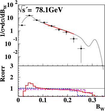
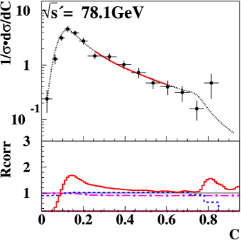
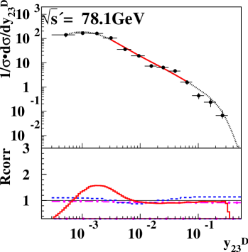
The region used in the fit is adjusted such that the background subtraction and the detector and hadronisation corrections are small (less than 50%) and uniform in that region. The resulting fit ranges are mainly restricted by the hadronisation corrections. The QCD predictions at $\sqrt{s^{\prime}}=78$ GeV fitted to data after applying the hadronisation correction are shown in Figure 6. Good agreement between data and theory is seen. The fitted values of $\alpha_{s}$ and their errors for each event shape observable are shown in Tables 2-5.

6.1 Systematic Uncertainties

6.1.1 Experimental Uncertainties

The experimental uncertainty is estimated by adding in quadrature the following contributions:

• the difference between the standard result and the result when all clusters and tracks are used without correcting for double counting of energy. This variation is sensitive to imperfections of the detector simulation.

• the largest deviation between the standard result and the result when the analysis is repeated with tighter selection criteria to eliminate background (standard values in brackets): the thrust axis is required to lie in the range $|\cos{\theta_{T}}|<0.7$ (0.9), or the cluster shape variable is required to be smaller than 5 (10), or the isolation angle from any jet is required to be larger than $35^{\circ}$ ($25^{\circ}$).

• the difference between the standard value and the value obtained by repeating the analysis with the background fractions estimated from the rate of isolated charged hadrons as described in Section 4.

• the difference between the standard result and the result when the single block energy resolution is varied to give the expected $\chi^{2}$ in the cluster shape fits. This check is made, because the values of $\chi^{2}$ in the cluster shape fits depend on the assumed energy resolution.

• the maximum difference between the standard result and the result when the fit regions are varied. The lower and upper limit of the fitting region are independently changed by $\pm 1$ bin.

The tighter selection on $|\cos{\theta_{T}}|$ and the alternative single block energy resolution of the electromagnetic calorimeter yield the largest contributions to the experimental systematic uncertainty. The overall resolution and energy scale uncertainty of the electromagnetic calorimeter have a neglegible effect on the results of this analysis.

6.1.2 Hadronisation Uncertainties

The following variations are performed in order to estimate the hadronisation uncertainties:

• the largest of the changes in $\alpha_{s}$ observed when independently varying the hadronisation parameters $b$ and $\sigma_{Q}$ by $\pm 1$ standard deviation about their tuned values in JETSET [25];

• the change observed when the parton virtuality cut-off parameter $Q_{0}$ is varied by $\pm 1$ standard deviation about its tuned value in JETSET;

• the change observed when only the light quarks u, d, s and c are considered at the parton level in order to estimate potential quark mass effects;

• the differences with respect to the standard result when HERWIG or ARIADNE are used for the hadronisation correction, rather than JETSET.

We define the hadronisation correction uncertainty by adding in quadrature the deviation when using only light quarks and the larger deviation when using HERWIG or ARIADNE to calculate the corrections. These variations are observed to lead to larger differences than all other variations, i.e. the main contributions to the hadronisation uncertainties are the choice of hadronisation model and the potential effect of quark masses.

6.1.3 Theoretical Uncertainties

We fix the renormalisation scale parameter $x_{\mu}\equiv\mu/Q$ to 1, where $\mu$ is the energy scale at which the theory is renormalized and $Q$ is the energy scale of the reaction. Although the uncertainty on the choice of the value of $x_{\mu}$ gives a large contribution to the systematic uncertainty, the means of quantifying this uncertainty is essentially arbitrary. We define the scale uncertainty as the larger of the deviations of $\alpha_{s}$ when $x_{\mu}$ is changed from 1 to 0.5 or 2.0.

The O($\alpha_{s}^{2}$) and NLLA calculations are combined with the ln(R) matching scheme. The variation in $\alpha_{s}(\sqrt{s^{\prime}}$) due to using different matching schemes is much smaller than the renormalisation scale uncertainty [48], and is not included as an additional theoretical systematic uncertainty.

6.2 Combination of $\alpha_{s}$ Results

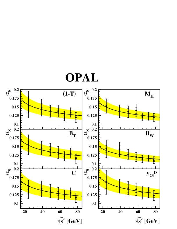
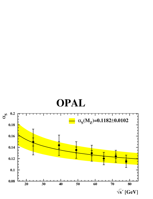
The values of $\alpha_{s}$ obtained for each observable at each energy are used to study the energy dependence of $\alpha_{s}$ and to obtain an overall combined result for $\alpha_{s}(M_{\mathrm{Z}})$. The individual values of $\alpha_{s}$ as given in Tables 2-5 and shown in Figure 7 are combined taking the correlations between their statistical and systematic errors into account using the method described in [8]. The statistical covariances between results from different observables are determined at each energy from 100 Monte Carlo subsamples with the same number of events as selected in the data. The experimental systematic uncertainties are assumed to be partially correlated, i.e. $cov_{ij}=\min(\sigma_{i},\sigma_{j})^{2}$. The hadronisation and theoretical covariances are only added to the diagonal of the total covariance matrix. The correlations between these uncertainties are considered by repeating the combination procedure with different hadronisation corrections (udsc only, HERWIG, ARIADNE) and with different renormalisation scale parameters ($x_{\mu}=2$ and 0.5). The systematic uncertainties for the combined value are obtained by repeating the combination for each systematic variation. The resulting values of $\alpha_{s}(\sqrt{s^{\prime}}$) are shown in Table 6 and Figure 8.

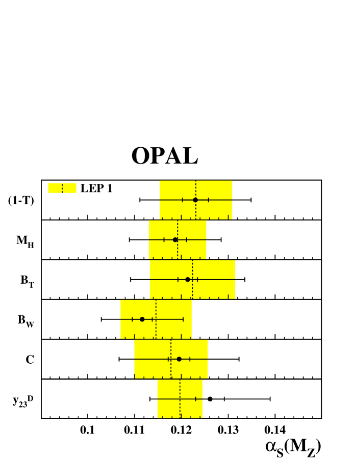
Values of $\alpha_{s}$ from individual observables at each energy are combined after evolving them to $\sqrt{s}=M_{\mathrm{Z}}$. In this case the results are statistically uncorrelated. The correlations between systematic uncertainties are treated as explained above. The results are given in Table 7 and Figure 9.

We also combine the combined values listed in Table 7 taking into account their statistical correlations using the sum of the inverses of the individual statistical covariance matrices at each energy point. The result is

$$\alpha_{s}(M_{\mathrm{Z}})=0.1182\pm 0.0015(\mathrm{stat.})\pm 0.0101(\mathrm{syst.}).$$ (8)

and is shown with individual errors in Table 7. Figure 8 shows the evolution of the strong coupling using our result. As a crosscheck on the robustness of the combination procedure we repeat the combination using the combined results at each energy point shown in Table 6 or using all individual results and find $\alpha_{s}(M_{\mathrm{Z}})=0.1183\pm 0.0103$ or $\alpha_{s}(M_{\mathrm{Z}})=0.1179\pm 0.0103$, respectively.

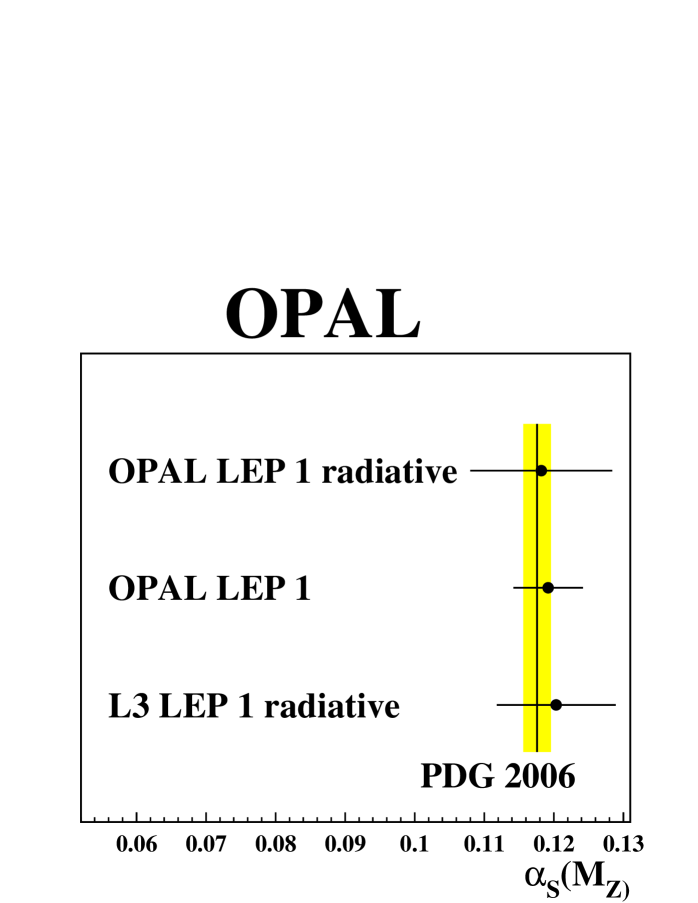
Our result is consistent within the statistical and experimental errors with the result from OPAL using non-radiative events in LEP 1 data with the same set of observables, $\alpha_{s}(M_{\mathrm{Z}})=0.1192\pm 0.0002(\mathrm{stat.})\pm 0.0050(\mathrm{syst.})$ [8]. Our result is also consistent with recent combined values [51, 11, 50, 49] and results from other analyses using radiative events [16, 17]. Figure 10 compares our result with the LEP 1 value for $\alpha_{s}$ from [8] and an average of results from L3 using radiative hadronic $\mathrm{Z}^{0}$ decays [16].

The combinations of individual observables at different cms energies yield $\chi^{2}/\mathrm{d.o.f.}\approx 1/6$. The small values of $\chi^{2}/\mathrm{d.o.f.}$ are due to the conservative treatment of hadronisation and theoretical uncertainties. The values of $\chi^{2}/\mathrm{d.o.f.}$ indicate consistency of the individual results with the model of the combination including evolution of results at different cms energies to $M_{\mathrm{Z}}$ before the combination.

7 Summary

The strong coupling $\alpha_{s}$ has been measured at reduced cms energies, $\sqrt{s^{\prime}}$, ranging from 20 GeV to 80 GeV using event shape observables derived from the hadronic system in radiative hadronic events.

Fits of O($\alpha_{s}^{2}$) and NLLA QCD predictions to the six event shape observables $1-T$, $M_{H}$, $B_{T}$, $B_{W}$, $C$ and $y_{23}^{D}$ are performed and values of $\alpha_{s}$ are obtained for seven values of $\sqrt{s^{\prime}}$. Our results are consistent with the running of $\alpha_{s}$ as predicted by QCD. The values at each $\sqrt{s^{\prime}}$ are evolved to $\mu=M_{\mathrm{Z}}$ and combined for each event shape observable. The combined value from all event shape observables and $\sqrt{s^{\prime}}$ values is $\alpha_{s}(M_{\mathrm{Z}})=0.1182\pm 0.0015(\mathrm{stat.})\pm 0.0101(\mathrm{syst.})$.

This result agrees with previous OPAL analyses with non-radiative LEP 1 data, with a similar measurement by L3, and with recent world average values, see figure 10. Within errors, QCD is consistent with our data sample of events with isolated FSR. Our result supports the assumption that the effects of high energy and large angle FSR on event shapes in hadronic $\mathrm{Z}^{0}$ decays can be effectively described by QCD with a lower effective cms energy $\sqrt{s^{\prime}}$.

$E_{\gamma}$ [GeV]	Events	$\sqrt{s^{\prime}}_{Mean}$[GeV]	Background [$\%$]
			Non-rad. MH		$\tau\tau$
			Likelihood	Isolated tracks
10-15	1560	78.1$\pm$ 1.7	6.0$\pm$ 0.7	6.2$\pm$ 0.9	0.9$\pm$ 0.2
15-20	954	71.8$\pm$ 1.9	3.1$\pm$ 0.5	4.9$\pm$ 0.8	1.0$\pm$ 0.3
20-25	697	65.1$\pm$ 2.0	2.6$\pm$ 0.6	6.3$\pm$ 1.1	0.9$\pm$ 0.4
25-30	513	57.6$\pm$ 2.3	5.1$\pm$ 1.1	7.9$\pm$ 1.4	1.1$\pm$ 0.5
30-35	453	49.0$\pm$ 2.6	4.5$\pm$ 1.1	9.6$\pm$ 1.6	0.7$\pm$ 0.4
35-40	376	38.5$\pm$ 3.5	5.2$\pm$ 1.2	13.1$\pm$ 1.9	0.8$\pm$ 0.5
40-45	290	24.4$\pm$ 5.3	10.4$\pm$ 2.3	12.9$\pm$ 1.7	0.8$\pm$ 0.5

Table 1: The number of selected events and the mean value of $\sqrt{s^{\prime}}$ for each $\sqrt{s^{\prime}}$ subsample. The neutral hadron background fractions estimated by the two methods described in Section 4.4 are listed in the columns “Non-rad. MH”.

	$(1-T)$	$M_{H}$	$B_{T}$	$B_{W}$	$C$	$y_{23}^{D}$
$\alpha_{s}(78.1\mathrm{GeV})$	0.1194	0.1193	0.1144	0.1103	0.1162	0.1225
Statistical Error	$\pm$ 0.0052	$\pm$ 0.0047	$\pm$ 0.0032	$\pm$ 0.0039	$\pm$ 0.0045	$\pm$ 0.0050
$\rm{Tracks+Clusters}$	$0.0005$	$-0.0005$	$-0.0000$	$-0.0009$	$0.0002$	$0.0012$
$|\cos{\theta_{T}}|<0.7$	$0.0096$	$0.0074$	$0.0059$	$0.0063$	$0.0067$	$0.0080$
$C>5$	$0.0012$	$0.0001$	$0.0005$	$-0.0004$	$0.0009$	$0.0006$
$\alpha^{\mathrm{iso}}_{j}$	$0.0000$	$0.0003$	$0.0027$	$0.0010$	$0.0004$	$-0.0012$
$\rm{Bkg\ fraction}$	$-0.0001$	$-0.0001$	$-0.0001$	$-0.0001$	$-0.0001$	$-0.0000$
$\rm{ECAL\ Resolution}$	$0.0018$	$0.0004$	$0.0004$	$0.0005$	$0.0011$	$-0.0005$
$\rm{Fitting\ Range}$	$0.0022$	$0.0005$	$0.0007$	$0.0016$	$0.0005$	$0.0005$
Experimental Syst.	$\pm$ 0.0101	$\pm$ 0.0075	$\pm$ 0.0066	$\pm$ 0.0066	$\pm$ 0.0069	$\pm$ 0.0082
$b-1s.d.$	$-0.0005$	$-0.0006$	$-0.0004$	$-0.0002$	$-0.0006$	$-0.0004$
$b+1s.d.$	$0.0004$	$0.0005$	$0.0005$	$0.0002$	$0.0007$	$0.0003$
$Q_{0}-1s.d.$	$0.0002$	$-0.0004$	$0.0006$	$-0.0003$	$0.0005$	$-0.0013$
$Q_{0}+1s.d.$	$-0.0002$	$0.0005$	$-0.0005$	$0.0003$	$-0.0002$	$0.0010$
$\sigma_{q}-1s.d.$	$0.0004$	$0.0003$	$0.0005$	$0.0003$	$0.0007$	$0.0007$
$\sigma_{q}+1s.d.$	$-0.0005$	$-0.0000$	$-0.0005$	$-0.0003$	$-0.0007$	$-0.0005$
$\rm{udsc\ only}$	$0.0021$	$-0.0001$	$0.0056$	$0.0023$	$0.0036$	$0.0065$
$\rm{Herwig\ 5.9}$	$-0.0053$	$-0.0046$	$-0.0064$	$-0.0042$	$-0.0082$	$-0.0078$
$\rm{Ariadne\ 4.08}$	$0.0000$	$-0.0015$	$-0.0017$	$-0.0001$	$-0.0023$	$-0.0033$
Total Hadronisation	$\pm$ 0.0057	$\pm$ 0.0049	$\pm$ 0.0087	$\pm$ 0.0048	$\pm$ 0.0093	$\pm$ 0.0108
$x_{\mu}=0.5$	$-0.0051$	$-0.0039$	$-0.0052$	$-0.0030$	$-0.0053$	$-0.0009$
$x_{\mu}=2.0$	$0.0065$	$0.0054$	$0.0065$	$0.0043$	$0.0067$	$0.0039$
Total error	$+$ 0.0143	$+$ 0.0115	$+$ 0.0131	$+$ 0.0100	$+$ 0.0141	$+$ 0.0150
	$-$ 0.0137	$-$ 0.0108	$-$ 0.0125	$-$ 0.0095	$-$ 0.0136	$-$ 0.0145

	$(1-T)$	$M_{H}$	$B_{T}$	$B_{W}$	$C$	$y_{23}^{D}$
$\alpha_{s}(71.8\mathrm{GeV})$	0.1336	0.1225	0.1304	0.1161	0.1305	0.1313
Statistical Error	$\pm$ 0.0062	$\pm$ 0.0048	$\pm$ 0.0039	$\pm$ 0.0054	$\pm$ 0.0058	$\pm$ 0.0065
$\rm{Tracks+Clusters}$	$0.0002$	$0.0002$	$-0.0000$	$0.0001$	$-0.0005$	$0.0009$
$|\cos{\theta_{T}}|<0.7$	$0.0028$	$0.0054$	$0.0005$	$0.0008$	$-0.0024$	$-0.0005$
$C>5$	$0.0003$	$0.0010$	$-0.0003$	$-0.0007$	$-0.0008$	$-0.0011$
$\alpha^{\mathrm{iso}}_{j}$	$-0.0031$	$-0.0021$	$-0.0022$	$-0.0008$	$-0.0025$	$-0.0043$
$\rm{Bkg\ fraction}$	$0.0000$	$0.0001$	$0.0000$	$0.0001$	$0.0001$	$0.0000$
$\rm{ECAL\ Resolution}$	$0.0015$	$0.0022$	$0.0014$	$0.0023$	$0.0007$	$0.0027$
$\rm{Fitting\ Range}$	$0.0020$	$0.0007$	$0.0007$	$0.0018$	$0.0004$	$0.0009$
Experimental Syst.	$\pm$ 0.0049	$\pm$ 0.0064	$\pm$ 0.0028	$\pm$ 0.0032	$\pm$ 0.0037	$\pm$ 0.0054
$b-1s.d.$	$-0.0006$	$-0.0005$	$-0.0005$	$-0.0001$	$-0.0006$	$-0.0004$
$b+1s.d.$	$0.0005$	$0.0005$	$0.0004$	$0.0002$	$0.0005$	$0.0002$
$Q_{0}-1s.d.$	$0.0002$	$-0.0005$	$0.0007$	$-0.0003$	$0.0003$	$-0.0017$
$Q_{0}+1s.d.$	$-0.0004$	$0.0003$	$-0.0007$	$0.0003$	$-0.0003$	$0.0011$
$\sigma_{q}-1s.d.$	$0.0004$	$0.0002$	$0.0005$	$0.0003$	$0.0005$	$0.0004$
$\sigma_{q}+1s.d.$	$-0.0005$	$-0.0002$	$-0.0005$	$-0.0003$	$-0.0005$	$-0.0006$
$\rm{udsc\ only}$	$0.0023$	$-0.0000$	$0.0061$	$0.0021$	$0.0033$	$0.0060$
$\rm{Herwig\ 5.9}$	$-0.0063$	$-0.0049$	$-0.0072$	$-0.0041$	$-0.0084$	$-0.0088$
$\rm{Ariadne\ 4.08}$	$-0.0002$	$-0.0018$	$-0.0017$	$-0.0002$	$-0.0015$	$-0.0034$
Total Hadronisation	$\pm$ 0.0067	$\pm$ 0.0053	$\pm$ 0.0096	$\pm$ 0.0046	$\pm$ 0.0092	$\pm$ 0.0113
$x_{\mu}=0.5$	$-0.0071$	$-0.0043$	$-0.0075$	$-0.0034$	$-0.0074$	$-0.0017$
$x_{\mu}=2.0$	$0.0091$	$0.0060$	$0.0094$	$0.0049$	$0.0093$	$0.0049$
Total error	$+$ 0.0138	$+$ 0.0113	$+$ 0.0143	$+$ 0.0092	$+$ 0.0147	$+$ 0.0150
	$-$ 0.0126	$-$ 0.0105	$-$ 0.0131	$-$ 0.0085	$-$ 0.0136	$-$ 0.0142

Table 2: Values of $\alpha_{s}$ and their errors for subsamples $E_{\gamma}$=10-15 GeV (upper) and 15-20 GeV (lower).

	$(1-T)$	$M_{H}$	$B_{T}$	$B_{W}$	$C$	$y_{23}^{D}$
$\alpha_{s}(65.1\mathrm{GeV})$	0.1236	0.1208	0.1217	0.1135	0.1242	0.1311
Statistical Error	$\pm$ 0.0068	$\pm$ 0.0063	$\pm$ 0.0058	$\pm$ 0.0053	$\pm$ 0.0059	$\pm$ 0.0133
$\rm{Tracks+Clusters}$	$-0.0011$	$0.0019$	$0.0020$	$-0.0007$	$-0.0016$	$-0.0014$
$|\cos{\theta_{T}}|<0.7$	$0.0043$	$0.0052$	$0.0052$	$0.0018$	$0.0009$	$-0.0041$
$C>5$	$0.0021$	$0.0001$	$0.0002$	$0.0016$	$-0.0010$	$0.0009$
$\alpha^{\mathrm{iso}}_{j}$	$0.0022$	$0.0012$	$0.0016$	$0.0022$	$0.0008$	$0.0005$
$\rm{Bkg\ fraction}$	$0.0001$	$0.0000$	$0.0000$	$0.0000$	$0.0000$	$0.0000$
$\rm{ECAL\ Resolution}$	$-0.0002$	$0.0000$	$0.0008$	$0.0007$	$0.0010$	$0.0013$
$\rm{Fitting\ Range}$	$0.0025$	$0.0010$	$0.0007$	$0.0014$	$0.0006$	$0.0017$
Experimental Syst.	$\pm$ 0.0059	$\pm$ 0.0057	$\pm$ 0.0059	$\pm$ 0.0037	$\pm$ 0.0025	$\pm$ 0.0049
$b-1s.d.$	$-0.0007$	$-0.0006$	$-0.0005$	$-0.0003$	$-0.0008$	$-0.0002$
$b+1s.d.$	$0.0005$	$0.0007$	$0.0002$	$0.0003$	$0.0008$	$0.0004$
$Q_{0}-1s.d.$	$0.0002$	$-0.0005$	$0.0005$	$-0.0004$	$0.0004$	$-0.0017$
$Q_{0}+1s.d.$	$-0.0003$	$0.0004$	$-0.0006$	$0.0003$	$-0.0002$	$0.0015$
$\sigma_{q}-1s.d.$	$0.0005$	$0.0003$	$0.0004$	$0.0003$	$0.0008$	$0.0007$
$\sigma_{q}+1s.d.$	$-0.0007$	$-0.0003$	$-0.0005$	$-0.0004$	$-0.0009$	$-0.0005$
$\rm{udsc\ only}$	$0.0021$	$0.0001$	$0.0039$	$0.0025$	$0.0034$	$0.0062$
$\rm{Herwig\ 5.9}$	$-0.0067$	$-0.0051$	$-0.0060$	$-0.0057$	$-0.0096$	$-0.0099$
$\rm{Ariadne\ 4.08}$	$-0.0007$	$-0.0025$	$-0.0007$	$-0.0009$	$-0.0027$	$-0.0040$
Total Hadronisation	$\pm$ 0.0071	$\pm$ 0.0057	$\pm$ 0.0072	$\pm$ 0.0063	$\pm$ 0.0106	$\pm$ 0.0125
$x_{\mu}=0.5$	$-0.0057$	$-0.0042$	$-0.0061$	$-0.0034$	$-0.0064$	$-0.0014$
$x_{\mu}=2.0$	$0.0073$	$0.0058$	$0.0076$	$0.0048$	$0.0081$	$0.0048$
Total error	$+$ 0.0136	$+$ 0.0117	$+$ 0.0134	$+$ 0.0102	$+$ 0.0148	$+$ 0.0195
	$-$ 0.0128	$-$ 0.0111	$-$ 0.0126	$-$ 0.0096	$-$ 0.0140	$-$ 0.0190

	$(1-T)$	$M_{H}$	$B_{T}$	$B_{W}$	$C$	$y_{23}^{D}$
$\alpha_{s}(57.6\mathrm{GeV})$	0.1378	0.1396	0.1327	0.1194	0.1284	0.1407
Statistical Error	$\pm$ 0.0085	$\pm$ 0.0094	$\pm$ 0.0072	$\pm$ 0.0064	$\pm$ 0.0063	$\pm$ 0.0091
$\rm{Tracks+Clusters}$	$0.0004$	$0.0022$	$-0.0008$	$0.0005$	$0.0039$	$-0.0013$
$|\cos{\theta_{T}}|<0.7$	$0.0065$	$0.0101$	$0.0078$	$0.0054$	$0.0083$	$0.0056$
$C>5$	$-0.0003$	$0.0020$	$0.0013$	$0.0013$	$0.0005$	$0.0009$
$\alpha^{\mathrm{iso}}_{j}$	$-0.0010$	$-0.0052$	$0.0004$	$-0.0004$	$0.0001$	$-0.0007$
$\rm{Bkg\ fraction}$	$0.0000$	$0.0000$	$0.0000$	$0.0000$	$0.0000$	$0.0000$
$\rm{ECAL\ Resolution}$	$0.0032$	$0.0051$	$0.0035$	$0.0021$	$0.0010$	$-0.0013$
$\rm{Fitting\ Range}$	$0.0036$	$0.0006$	$0.0014$	$0.0020$	$0.0011$	$0.0010$
Experimental Syst.	$\pm$ 0.0082	$\pm$ 0.0128	$\pm$ 0.0088	$\pm$ 0.0063	$\pm$ 0.0093	$\pm$ 0.0061
$b-1s.d.$	$-0.0009$	$-0.0004$	$-0.0005$	$-0.0003$	$-0.0010$	$-0.0006$
$b+1s.d.$	$0.0006$	$0.0004$	$0.0004$	$0.0004$	$0.0009$	$0.0005$
$Q_{0}-1s.d.$	$0.0002$	$-0.0008$	$0.0006$	$-0.0005$	$0.0005$	$-0.0023$
$Q_{0}+1s.d.$	$-0.0005$	$0.0005$	$-0.0009$	$0.0003$	$-0.0004$	$0.0016$
$\sigma_{q}-1s.d.$	$0.0005$	$0.0002$	$0.0005$	$0.0006$	$0.0009$	$0.0006$
$\sigma_{q}+1s.d.$	$-0.0009$	$-0.0002$	$-0.0005$	$-0.0004$	$-0.0010$	$-0.0007$
$\rm{udsc\ only}$	$0.0024$	$-0.0001$	$0.0042$	$0.0033$	$0.0040$	$0.0063$
$\rm{Herwig\ 5.9}$	$-0.0076$	$-0.0039$	$-0.0072$	$-0.0066$	$-0.0101$	$-0.0113$
$\rm{Ariadne\ 4.08}$	$-0.0011$	$-0.0011$	$-0.0012$	$-0.0013$	$-0.0032$	$-0.0049$
Total Hadronisation	$\pm$ 0.0081	$\pm$ 0.0041	$\pm$ 0.0085	$\pm$ 0.0075	$\pm$ 0.0114	$\pm$ 0.0140
$x_{\mu}=0.5$	$-0.0079$	$-0.0063$	$-0.0078$	$-0.0042$	$-0.0072$	$-0.0023$
$x_{\mu}=2.0$	$0.0101$	$0.0087$	$0.0098$	$0.0058$	$0.0090$	$0.0063$
Total error	$+$ 0.0175	$+$ 0.0186	$+$ 0.0172	$+$ 0.0130	$+$ 0.0183	$+$ 0.0189
	$-$ 0.0164	$-$ 0.0176	$-$ 0.0162	$-$ 0.0124	$-$ 0.0175	$-$ 0.0180

Table 3: Values of $\alpha_{s}$ and their errors for subsamples $E_{\gamma}=20-25$ GeV (upper) and $25-30$ GeV (lower).

	$(1-T)$	$M_{H}$	$B_{T}$	$B_{W}$	$C$	$y_{23}^{D}$
$\alpha_{s}(49.0\mathrm{GeV})$	0.1373	0.1359	0.1413	0.1269	0.1356	0.1440
Statistical Error	$\pm$ 0.0105	$\pm$ 0.0098	$\pm$ 0.0087	$\pm$ 0.0069	$\pm$ 0.0089	$\pm$ 0.0117
$\rm{Tracks+Clusters}$	$0.0022$	$0.0007$	$0.0032$	$-0.0003$	$0.0008$	$-0.0012$
$|\cos{\theta_{T}}|<0.7$	$0.0029$	$0.0039$	$0.0004$	$0.0012$	$-0.0001$	$-0.0000$
$C>5$	$-0.0010$	$-0.0038$	$-0.0017$	$-0.0001$	$-0.0049$	$-0.0018$
$\alpha^{\mathrm{iso}}_{j}$	$0.0024$	$0.0024$	$0.0007$	$0.0017$	$0.0013$	$0.0046$
$\rm{Bkg\ fraction}$	$0.0001$	$0.0000$	$0.0001$	$0.0000$	$0.0000$	$0.0001$
$\rm{ECAL\ Resolution}$	$-0.0003$	$0.0010$	$-0.0003$	$0.0009$	$-0.0000$	$-0.0005$
$\rm{Fitting\ Range}$	$0.0027$	$0.0013$	$0.0009$	$0.0016$	$0.0009$	$0.0020$
Experimental Syst.	$\pm$ 0.0053	$\pm$ 0.0062	$\pm$ 0.0038	$\pm$ 0.0028	$\pm$ 0.0052	$\pm$ 0.0055
$b-1s.d.$	$-0.0005$	$-0.0009$	$-0.0006$	$-0.0005$	$-0.0009$	$-0.0008$
$b+1s.d.$	$0.0005$	$0.0008$	$0.0003$	$0.0005$	$0.0007$	$0.0002$
$Q_{0}-1s.d.$	$0.0003$	$-0.0006$	$0.0006$	$-0.0003$	$0.0005$	$-0.0019$
$Q_{0}+1s.d.$	$-0.0005$	$0.0005$	$-0.0012$	$0.0004$	$-0.0005$	$0.0017$
$\sigma_{q}-1s.d.$	$0.0005$	$0.0005$	$0.0004$	$0.0007$	$0.0007$	$0.0007$
$\sigma_{q}+1s.d.$	$-0.0006$	$-0.0006$	$-0.0008$	$-0.0007$	$-0.0009$	$-0.0006$
$\rm{udsc\ only}$	$0.0023$	$0.0002$	$0.0039$	$0.0050$	$0.0038$	$0.0060$
$\rm{Herwig\ 5.9}$	$-0.0083$	$-0.0090$	$-0.0080$	$-0.0083$	$-0.0123$	$-0.0114$
$\rm{Ariadne\ 4.08}$	$-0.0009$	$-0.0041$	$-0.0011$	$-0.0024$	$-0.0039$	$-0.0056$
Total Hadronisation	$\pm$ 0.0087	$\pm$ 0.0099	$\pm$ 0.0091	$\pm$ 0.0101	$\pm$ 0.0135	$\pm$ 0.0142
$x_{\mu}=0.5$	$-0.0076$	$-0.0058$	$-0.0092$	$-0.0054$	$-0.0081$	$-0.0008$
$x_{\mu}=2.0$	$0.0097$	$0.0081$	$0.0117$	$0.0072$	$0.0102$	$0.0056$
Total error	$+$ 0.0176	$+$ 0.0173	$+$ 0.0176	$+$ 0.0144	$+$ 0.0198	$+$ 0.0201
	$-$ 0.0165	$-$ 0.0163	$-$ 0.0160	$-$ 0.0136	$-$ 0.0188	$-$ 0.0193

	$(1-T)$	$M_{H}$	$B_{T}$	$B_{W}$	$C$	$y_{23}^{D}$
$\alpha_{s}(38.5\mathrm{GeV})$	0.1474	0.1374	0.1451	0.1415	0.1421	0.1496
Statistical Error	$\pm$ 0.0125	$\pm$ 0.0112	$\pm$ 0.0088	$\pm$ 0.0113	$\pm$ 0.0113	$\pm$ 0.0101
$\rm{Tracks+Clusters}$	$0.0024$	$0.0019$	$0.0006$	$0.0001$	$0.0049$	$-0.0010$
$|\cos{\theta_{T}}|<0.7$	$0.0026$	$0.0059$	$0.0034$	$0.0061$	$0.0050$	$0.0022$
$C>5$	$0.0042$	$0.0038$	$0.0018$	$0.0037$	$0.0052$	$0.0040$
$\alpha^{\mathrm{iso}}_{j}$	$0.0005$	$-0.0007$	$-0.0004$	$0.0043$	$0.0014$	$0.0026$
$\rm{Bkg\ fraction}$	$0.0003$	$0.0003$	$0.0002$	$0.0002$	$0.0003$	$0.0004$
$\rm{ECAL\ Resolution}$	$0.0019$	$0.0025$	$0.0003$	$0.0035$	$0.0039$	$0.0055$
$\rm{Fitting\ Range}$	$0.0033$	$0.0009$	$0.0008$	$0.0013$	$0.0023$	$0.0008$
Experimental Syst.	$\pm$ 0.0067	$\pm$ 0.0077	$\pm$ 0.0040	$\pm$ 0.0092	$\pm$ 0.0099	$\pm$ 0.0077
$b-1s.d.$	$-0.0009$	$-0.0007$	$-0.0007$	$-0.0004$	$-0.0007$	$-0.0005$
$b+1s.d.$	$0.0009$	$0.0006$	$0.0006$	$0.0005$	$0.0005$	$0.0004$
$Q_{0}-1s.d.$	$0.0006$	$-0.0008$	$0.0011$	$-0.0008$	$0.0007$	$-0.0021$
$Q_{0}+1s.d.$	$-0.0005$	$0.0008$	$-0.0014$	$0.0006$	$-0.0007$	$0.0018$
$\sigma_{q}-1s.d.$	$0.0013$	$0.0003$	$0.0008$	$0.0006$	$0.0010$	$0.0005$
$\sigma_{q}+1s.d.$	$-0.0009$	$-0.0002$	$-0.0008$	$-0.0004$	$-0.0007$	$-0.0006$
$\rm{udsc\ only}$	$0.0042$	$0.0001$	$0.0060$	$0.0036$	$0.0038$	$0.0064$
$\rm{Herwig\ 5.9}$	$-0.0150$	$-0.0096$	$-0.0105$	$-0.0107$	$-0.0125$	$-0.0127$
$\rm{Ariadne\ 4.08}$	$-0.0042$	$-0.0036$	$-0.0028$	$-0.0025$	$-0.0030$	$-0.0055$
Total Hadronisation	$\pm$ 0.0162	$\pm$ 0.0103	$\pm$ 0.0125	$\pm$ 0.0116	$\pm$ 0.0135	$\pm$ 0.0154
$x_{\mu}=0.5$	$-0.0093$	$-0.0055$	$-0.0097$	$-0.0072$	$-0.0089$	$-0.0012$
$x_{\mu}=2.0$	$0.0120$	$0.0079$	$0.0124$	$0.0097$	$0.0114$	$0.0063$
Total error	$+$ 0.0247	$+$ 0.0188	$+$ 0.0201	$+$ 0.0210	$+$ 0.0232	$+$ 0.0210
	$-$ 0.0235	$-$ 0.0179	$-$ 0.0186	$-$ 0.0199	$-$ 0.0221	$-$ 0.0200

Table 4: Values of $\alpha_{s}$ and their errors for subsamples $E_{\gamma}=30-35$ GeV (upper) and $35-40$ GeV (lower).

	$(1-T)$	$M_{H}$	$B_{T}$	$B_{W}$	$C$	$y_{23}^{D}$
$\alpha_{s}(24.4\mathrm{GeV})$	0.1569	0.1524	0.1552	0.1433	0.1406	0.1612
Statistical Error	$\pm$ 0.0252	$\pm$ 0.0117	$\pm$ 0.0115	$\pm$ 0.0101	$\pm$ 0.0112	$\pm$ 0.0181
$\rm{Tracks+Clusters}$	$0.0038$	$0.0015$	$0.0060$	$-0.0021$	$0.0080$	$-0.0074$
$|\cos{\theta_{T}}|<0.7$	$0.0001$	$0.0008$	$-0.0027$	$0.0027$	$0.0013$	$-0.0008$
$C>5$	$0.0037$	$-0.0001$	$-0.0036$	$-0.0022$	$-0.0010$	$-0.0084$
$\alpha^{\mathrm{iso}}_{j}$	$0.0110$	$0.0056$	$0.0003$	$0.0023$	$0.0060$	$0.0005$
$\rm{Bkg\ fraction}$	$0.0023$	$0.0017$	$0.0018$	$0.0015$	$0.0020$	$0.0031$
$\rm{ECAL\ Resolution}$	$-0.0035$	$-0.0053$	$-0.0039$	$-0.0013$	$-0.0025$	$-0.0057$
$\rm{Fitting\ Range}$	$0.0035$	$0.0027$	$0.0018$	$0.0017$	$0.0020$	$0.0018$
Experimental Syst.	$\pm$ 0.0134	$\pm$ 0.0085	$\pm$ 0.0088	$\pm$ 0.0054	$\pm$ 0.0109	$\pm$ 0.0131
$b-1s.d.$	$-0.0007$	$-0.0014$	$-0.0007$	$-0.0013$	$-0.0012$	$-0.0013$
$b+1s.d.$	$0.0015$	$0.0017$	$0.0009$	$0.0011$	$0.0012$	$0.0006$
$Q_{0}-1s.d.$	$0.0010$	$-0.0010$	$0.0023$	$-0.0009$	$0.0010$	$-0.0039$
$Q_{0}+1s.d.$	$-0.0008$	$0.0004$	$-0.0029$	$0.0000$	$-0.0010$	$0.0015$
$\sigma_{q}-1s.d.$	$0.0014$	$0.0010$	$0.0011$	$0.0017$	$0.0012$	$0.0011$
$\sigma_{q}+1s.d.$	$-0.0010$	$-0.0009$	$-0.0010$	$-0.0018$	$-0.0013$	$-0.0016$
$\rm{udsc\ only}$	$0.0075$	$0.0053$	$0.0140$	$0.0159$	$0.0150$	$0.0168$
$\rm{Herwig\ 5.9}$	$-0.0212$	$-0.0080$	$-0.0134$	$-0.0126$	$-0.0103$	$-0.0193$
$\rm{Ariadne\ 4.08}$	$-0.0082$	$-0.0056$	$-0.0040$	$-0.0045$	$-0.0050$	$-0.0114$
Total Hadronisation	$\pm$ 0.0240	$\pm$ 0.0113	$\pm$ 0.0200	$\pm$ 0.0209	$\pm$ 0.0190	$\pm$ 0.0283
$x_{\mu}=0.5$	$-0.0104$	$-0.0085$	$-0.0116$	$-0.0082$	$-0.0088$	$-0.0024$
$x_{\mu}=2.0$	$0.0137$	$0.0115$	$0.0151$	$0.0108$	$0.0112$	$0.0084$
Total error	$+$ 0.0397	$+$ 0.0216	$+$ 0.0289	$+$ 0.0262	$+$ 0.0270	$+$ 0.0371
	$-$ 0.0387	$-$ 0.0202	$-$ 0.0273	$-$ 0.0252	$-$ 0.0261	$-$ 0.0362

Table 5: Values of $\alpha_{s}$ and their errors for subsample $E_{\gamma}=40-45$ GeV.

$\sqrt{s^{\prime}}$ [GeV]	78.1	71.8	65.1	57.6	49.0	38.5	24.4
$\alpha_{s}(\sqrt{s^{\prime}})$	0.1153	0.1242	0.1201	0.1296	0.1353	0.1438	0.1496
Statistical	0.0026	0.0037	0.0039	0.0047	0.0053	0.0064	0.0071
Experimental	0.0068	0.0036	0.0040	0.0069	0.0039	0.0063	0.0077
Hadronisation	0.0062	0.0065	0.0072	0.0085	0.0100	0.0122	0.0166
Theory	0.0053	0.0067	0.0063	0.0076	0.0086	0.0099	0.0117

Table 6: Combined values of $\alpha_{s}(\sqrt{s^{\prime}})$ and their errors from all event shape variables.

	$(1-T)$	$M_{H}$	$B_{T}$	$B_{W}$	$C$	$y_{23}^{D}$	Combined
$\alpha_{s}(M_{Z})$	0.1230	0.1187	0.1214	0.1117	0.1195	0.1261	0.1182
Statistical	0.0028	0.0024	0.0021	0.0021	0.0023	0.0031	0.0015
Experimental	0.0050	0.0054	0.0037	0.0033	0.0040	0.0049	0.0038
Hadronisation	0.0071	0.0052	0.0080	0.0061	0.0092	0.0105	0.0070
Theory	0.0076	0.0059	0.0081	0.0049	0.0076	0.0045	0.0062

Table 7: Combined values of $\alpha_{s}(M_{\mathrm{Z}})$ and their errors from all photon energy subsamples for a given observable. The final combined value of $\alpha_{s}(M_{\mathrm{Z}})$ is also shown.

$\mathbf{OPAL}$

Figure 1: The distributions of event shape observables $1-T$ and $M_{H}$ for non-radiative events and radiative hadronic events from the Monte Carlo generators JETSET, HERWIG and ARIADNE as indicated below the figures. The triangles and points show distributions obtained from the $\mathrm{Z}^{0}$ samples with FSR while the histograms show distributions from samples generated at lower energies as shown on the figure. The open triangles and solid histogram (solid points and dashed histogram) in each figure correspond to $\sqrt{s^{\prime}}=40$ (70) GeV.

$\mathbf{OPAL}$

Figure 2: Distributions of each variable used in the isolated photon selection. The error bars show the statistical errors. Monte Carlo distributions are normalized to the integrated luminosity of the data and the cross section of the process. Arrows in the figures show the selected region. Distributions for radiative multi-hadronic events, which are signal events in this analysis, are overlaid on distributions for all multi-hadronic events and $\tau\tau$ events. The distribution of each variable is obtained with the cuts on the preceeding variables applied.

$\mathbf{OPAL}$

Figure 3: Photon likelihood distributions. The error bar shows statistical error. The Monte Carlo distributions are normalised to the total number of candidates in the data, and the neutral hadron background fractions are obtained from the fits described in Section 4.4. The arrows indicate the selected regions.

$\mathbf{OPAL}$

Figure 4: Event shape distributions before background subtraction and detector correction. Two of the six event shape observables, $1-T$ and $M_{H}$, are shown for the low (38.5 GeV) and high (78.1 GeV) $\sqrt{s^{\prime}}$ samples. The histograms show Monte Carlo distributions. The error bars show the statistical errors.

$\mathbf{OPAL}$

Figure 5: Event shape distributions at the hadron level. The error bars correspond to the statistical and experimental uncertainties described in Section 6.1.1. Two of the six event shape observables, $1-T$ and $M_{H}$, are shown for the low (38.5 GeV) and high (78.1 GeV) $\sqrt{s^{\prime}}$ samples. The small lines on the error bars show the extent of the statistical uncertainty. The data points are placed at the centres of the corresponding bins. The predictions of JETSET, HERWIG and ARIADNE at the corresponding $\sqrt{s^{\prime}}$ values are also shown as lines.

$\mathbf{OPAL}$

Figure 6: Event shape distributions for data at $\langle\sqrt{s^{\prime}}\rangle=78.1$ GeV and the fitted theoretical predictions. The error bars show the statistical errors. The solid lines in the theoretical predictions show the regions used in the fit. Three corrections are plotted as “$R\mathrm{corr}$”: the detector correction, $r_{i}^{Det}$ (dashed line), the hadronisation correction, $R_{i}^{Had}$ (solid line), and the ratio of distributions after and before background subtraction (dotted line). The hadronisation correction is shown by the ratio of differential distributions in these figures (see text for details).

Figure 7: Energy dependence of $\alpha_{s}$ for all $\sqrt{s^{\prime}}$ subsamples. The inner error bars show the statistical and the outer error bars the total uncertainties. The curves and shaded bands show the QCD prediction for the running of $\alpha_{s}$ obtained with the corresponding values of $\alpha_{s}(M_{\mathrm{Z}})$ with total errors from Table 7.

Figure 8: Combined values of $\alpha_{s}$ from all event shape observables as shown in Table 6. The curve and shaded band show the QCD prediction for the running of $\alpha_{s}$ using the combined value of $\alpha_{s}(M_{\mathrm{Z}})$ with total errors.

Figure 9: The values of $\alpha_{s}(M_{\mathrm{Z}})$ obtained by combining all $\sqrt{s^{\prime}}$ samples as shown in Table 7. The inner error bars are statistical, the outer error bars correspond to the total uncertainty. The dashed vertical lines and shaded bands show the LEP 1 results from OPAL [8] using non-radiative events.

Figure 10: Combined values of $\alpha_{s}(M_{\mathrm{Z}})$ for all event shape observables and $\sqrt{s^{\prime}}$ samples. The error bars show total uncertainties. The results from this analyses with radiative events, from non-radiative events with OPAL LEP 1 data [8] and from L3 radiative events [16] are shown. The PDG [49] value of $\alpha_{s}(M_{\mathrm{Z}})$ is also shown as the vertical line, with the total uncertainty corresponding to the shaded band.

References

- [1] H. Fritzsch, M Gell-Mann and H. Leutwyler, Phys. Lett. B 47 (1973) 365.
- [2] D. J. Gross and F. Wilczek, Phys. Rev. Lett. 30 (1973) 1343.
- [3] H. D. Politzer, Phys. Rev. Lett. 30 (1973) 1346.
- [4] P. A. Movilla Fernandez, O. Biebel, S. Bethke, S. Kluth and P. Pfeifenschneider [JADE Coll.], Eur. Phys. J. C 1 (1998) 461.
- [5] P. Achard et al. [L3 Coll.], Phys. Rept. 399 (2004) 71.
- [6] A. Heister et al. [ALEPH Coll.], Eur. Phys. J. C 35 (2004) 457.
- [7] J. Abdallah et al. [DELPHI Coll.], Eur. Phys. J. C 37 (2004) 1.
- [8] G. Abbiendi et al. [OPAL Coll.], Eur. Phys. J. C 40 (2005) 287.
- [9] G. Abbiendi et al. [OPAL Coll.], Eur. Phys. J. C 47 (2006) 295.
- [10] J. Schieck et al. [JADE Coll.], Eur. Phys. J. C 48 (2006) 3.
- [11] S. Kluth, Rep. Prog. Phys. 69 (2006) 1771.
- [12] D. Leone et al. [KLOE Coll.], PoS (2005) 282.
- [13] A. Aloisio et al. [KLOE Coll.], Phys. Lett. B 606 (2005) 12.
- [14] A. Denig, Nucl. Phys. Proc. Suppl. 162 (2006) 81.
- [15] B. Aubert et al. [BaBar Coll.], Phys. Rev. D 70 (2004) 072004.
- [16] P. Achard et al. [L3 Coll.], Phys. Rept. B 597 (2004) 145.
- [17] J. Abdallah et al. [DELPHI Coll.], Eur. Phys. J. C 29 (2003) 285.
- [18] P. Abreu et al. [DELPHI Coll.], Z. Phys. C 70 (1996) 179.
- [19] T. Sjostrand, Comput. Phys. Commun. 82 (1994) 74.
- [20] G. Marchesini, B. R. Webber, G. Abbiendi, I. G. Knowles, M. H. Seymour and L. Stanco, Comput. Phys. Commun. 67 (1992) 465.
- [21] L. Lönnblad, Comput. Phys. Commun. 71 (1992) 15.
- [22] K. Abe et al. [SLD Coll.], Phys. Rev. D 59 (1999) 012002; G. Abbiendi et al. [OPAL Coll.], Eur. Phys. J. C 11 (1999) 643.
- [23] K. Ahmet et al. [OPAL Coll.], Nucl. Instrum. Meth. A 305 (1991) 275.
- [24] O. Biebel et al., Nucl. Instrum. Meth. A 323 (1992) 169.
- [25] G. Alexander et al. [OPAL Coll.], Z. Phys. C 69 (1996) 543.
- [26] K. Ackerstaff et al. [OPAL Coll.], Z. Phys. C 75 (1997) 193.
- [27] L. Lönnblad et al., hep-ph/9512371.
- [28] T. Sjostrand and F. Zwirner, in G. Altarelli ed., CERN 96-01, vol. 2 (1996) 187.
- [29] J. A. Vermaseren, Nucl. Phys. B 229 (1983) 347.
- [30] S. Jadach, B. F. Ward and Z. Was, Comput. Phys. Commun. 79 (1994) 503.
- [31] J. Allison et al. [OPAL Coll.], Nucl. Instrum. Meth. A 317 (1992) 47.
- [32] G. Alexander et al. [OPAL Coll.], Z. Phys. C 52 (1991) 175.
- [33] S. Catani, Y. L. Dokshitzer, M. Olsson, G. Turnock and B. R. Webber, Phys. Lett. B 269 (1991) 432.
- [34] D. Toya, Measurement of Strong Coupling Constant using Radiative Hadronic Events in Collision at LEP, Ph.D. thesis, Tokyo University (2003).
- [35] G. Abbiendi et al. [OPAL Coll.], Eur. Phys. J. C 32 (2004) 453.
- [36] D. Karlen, Computers in Physics, 12 (1998) 380.
- [37] K. Ackerstaff et al. [OPAL Coll.], Eur. Phys. J. C 5 (1998) 411; O. Adriani et al. [L3 Coll.], Phys. Lett. B 292 (1992) 472.
- [38] K. Ackerstaff et al. [OPAL Coll.], Eur. Phys. J. C 2 (1998) 213.
- [39] S. Catani, L. Trentadue, G. Turnock and B. R. Webber, Nucl. Phys. B 407 (1993) 3.
- [40] Y. L. Dokshitzer, A. Lucenti, G. Marchesini and G. P. Salam, JHEP 9801 (1998) 011.
- [41] S. Catani, G. Turnock and B. R. Webber, Phys. Lett. B 295 (1992) 269.
- [42] G. Parisi, Phys. Lett. B 74 (1978) 65.
- [43] J. F. Donoghue, F. E. Low and S. Y. Pi, Phys. Rev. D 20 (1979) 2759.
- [44] S. Bethke, Z. Kunszt, D. E. Soper and W. J. Stirling, Nucl. Phys. B 370 (1992) 310 (Erratum-ibid. B 523 (1998) 681).
- [45] N. Brown and W. J. Stirling, Z. Phys. C 53 (1992) 629.
- [46] G. Alexander et al. [OPAL Coll.], Z. Phys. C 72 (1996) 191.
- [47] K. Ackerstaff et al. [OPAL Coll.], Z. Phys. C 75 (1997) 193; G. Abbiendi et al. [OPAL Coll.], Eur. Phys. J. C 16 (2000) 185.
- [48] P. D. Acton et al. [OPAL Coll.], Z. Phys. C 59 (1993) 1.
- [49] W.-M. Yao et al. [Particle Data Group], J. Phys. G 33 (2006) 1.
- [50] S. Kluth, hep-ex/0609020 (2006), to appear in proceedings of XXXIII International Conference on High Energy Physics ICHEP 06, Moscow, Russia, Jul 16 to Aug 2 2006.
- [51] S. Bethke, Nucl. Phys. Proc. Suppl. 35 (2004) 345.