Characterizing the properties of Clusters of Galaxies as a function of luminosity and redshift

Abstract

We report the application of the new Monte Carlo method, Smoothed Particle Inference (SPI, described in a pair of companion papers), towards analysis and interpretation of X-ray observations of clusters of galaxies with the XMM-Newton satellite. Our sample consists of publicly available well-exposed observations of clusters at redshifts $z>0.069$, totaling 101 objects. We determine the luminosity and temperature structure of the X-ray emitting gas, with the goal to quantify the scatter and the evolution of the $L_{X}$ - $T$ relation, as well as to investigate the dependence on cluster substructure with redshift. This work is important for the establishment of the potential robustness of mass estimates from X-ray data which in turn is essential towards the use of clusters for measurements of cosmological parameters. We use the luminosity and temperature maps derived via the SPI technique to determine the presence of cooling cores, via measurements of luminosity and temperature contrast. The $L_{X}-T$ relation is investigated, and we confirm that $L_{X}\propto T^{3}$. We find a weak redshift dependence ($\propto(1+z)^{\beta_{LT}},\beta_{LT}=0.50\pm 0.34$), in contrast to some Chandra results. The level of dynamical activity is established using the “power ratios” method, and we compare our results to previous application of this method to Chandra data for clusters. We find signs of evolution in the $P_{3}/P_{0}$ power ratio. A new method, the “temperature two-point correlation function,” is proposed. This method is used to determine the “power spectrum” of temperature fluctuations in the X-ray emitting gas as a function of spatial scale. We show how this method can be fruitfully used to identify cooling core clusters as well as those with disturbed structures, presumably due to on-going or recent merger activity.

1. Introduction

Clusters of galaxies are the largest gravitationally bound structures in the Universe, and thus should provide a fair sample of its matter content. This makes clusters good candidates for cosmological studies. In particular, the gravitational growth of initial density perturbations can be used to constrain cosmological parameters via determination of the mass function of clusters of galaxies (e.g.  Voit, 2005), but this requires good knowledge of cluster masses.

One of the most promising avenues towards the measurement of the mass function of clusters is based on estimates of the cluster temperature and luminosity from X-ray observations of a large number of objects. Specifically, the number density for clusters of different masses can be estimated using mass-observable relations, calibrated using nearby clusters where spatially resolved spectroscopy is available. The mass-temperature ($M$-$T$) (e.g.  Arnaud et al., 2005) and luminosity-temperature ($L_{X}$-$T$) (e.g.  Arnaud & Evrard, 1999) scaling relations are of particular importance since temperature is often used as a proxy for mass and the relation to luminosity is needed to understand the sample selection function since X-ray selected samples generally are flux limited. More recently, a new proxy for cluster mass, $Y_{X}$, has been proposed (Kravtsov et al., 2006). This quantity is a simple product of the gas mass of the intra cluster medium and its temperature and has shown to exhibit a low amount of scatter.

Clusters are formed hierarchically through mergers of smaller clusters and groups. This merging activity is observed as distortions of their X-ray surface brightness profiles. Substructures and mergers affect the mass determinations and increase the scatter in the scaling relations. Measurements using only “relaxed” clusters have achieved high precision (Vikhlinin et al., 2006a) and selective studies, such as those of the gas mass fraction ($f_{gas}$) in clusters focus only on the largest clusters with minimal amount of substructure (Allen et al., 2008). However, substructure was found to be present in $\sim 50\%$ of clusters in a ROSAT study (Schuecker et al., 2001) and studies of XMM data in a REFLEX-DXL study find substructures present in all clusters in that sample (Finoguenov et al., 2005). Understanding, and assessing the effect of substructure on the robustness of mass determination is thus crucial.

Besides the complications associated with the merger activity, evolution of clusters can affect the applicability of scaling relations. The high density environments in galaxy cluster cores cause them to cool radiatively and this is observed in undisturbed clusters as a decrease of the average projected temperature towards the center (e.g.  Peterson & Fabian, 2006). The undisturbed “cooling clusters” have sharply peaked luminosity profiles, a feature that is not observed in their non-cooling counterparts. Cool-core clusters deviate from the $L_{X}$-$T$ relation since the core has higher luminosity and lower temperature than the cluster population on average. Observational evidence exists supporting the argument that cool cores can survive to some extent during a cluster merger. These core remnants are then observed as sharp contact discontinuities or “cold fronts” (e.g.  Markevitch & Vikhlinin, 2007), possibly affecting the $M$-$T$ scaling.

All this indicates that it is important to assess and quantify the dynamical state of a cluster when the cluster data are used for the determination of cosmological parameters. While this has been successfully attempted in the past (see e.g Maughan et al., 2008; Chen et al., 2007), statistical studies of cluster substructure have so far only used the information from the spatial distribution of X-ray counts on the sky, hence only mapping the luminosity structure. Ideally, the knowledge about the temperature structure should also be included in these searches since it holds important information about the dynamical history of the cluster.

The Smoothed Particle Inference (SPI) technique, developed recently by some of us (Peterson, Marshall, & Andersson, 2007) as an alternative to standard analysis techniques, is well suited for detecting the effects of cooling cores and substructure from both the projected temperature and luminosity distributions of clusters (see  Andersson et al., 2007). This method relies on a description of a cluster as a large set of smoothed particles (two-dimensional, spatial Gaussians), each of which is described by a luminosity, spatial position, Gaussian width, temperature, redshift, and a set of elemental abundances. A large set of these particles is propagated through an instrument model, and the model parameters are adjusted using Markov Chain methods. The resulting distribution becomes a kilo-parametric description of the cluster.

In this paper, the SPI method is used on a large number of cluster observations available through the XMM public archives. A cluster model is built using the the imaging spectroscopy XMM data. The output of the modeling is used to separate clusters with cooling cores from more disturbed clusters and to study their properties separately. Specifically, we aim to assess the effects of cooling cores and substructure on the luminosity-temperature relation and study any possible redshift dependence of these effects. We also apply a new statistic, including the spatial distribution of both luminosity and temperature to quantify the level of dynamical instability present in the clusters. This statistic is designed to distinguish cool core clusters and isothermal clusters from those with more temperature structure indicating a recent or ongoing merger event.

In Section 2 we describe the construction and properties of the cluster sample and outline the data reduction scheme, in Section 3 we explain the different methods used to analyze the data, and in Section 4 we describe the processing performed on the output cluster models and the methods used to quantify cluster properties. In Section 5 we display the statistical results of our modeling and in Section 6 we discuss the possible systematic effects associated with this. We finally conclude in Section 7 with a discussion on the results, problems and possible improvements.

In all calculations we have assumed a concordance cosmology with $\Omega_{M}=0.3$, $\Omega_{\Lambda}=0.7$ and $H_{0}=70~{}$km s${}^{-1}~{}$Mpc^-1.

2. Cluster sample and data preparation

The cluster sample was compiled by cross-correlating the NASA Extragalactic Database (NED) with the public XMM-Newton observation archive as of May 10, 2006. The requirement for selection in NED was that the cluster should be a known X-ray source and a known galaxy cluster (2005 clusters) or group (120 groups). The XMM pointing was required to be within $3.5^{\prime}$ of the source position in NED. This resulted in 278 matches for clusters and 34 for groups, some of which were multiple matches of the same cluster. After multiples and sources not visible in the X-ray data were removed the total number of clusters and groups was 201. We further removed clusters where we could not get a reliable spectrum, i.e. clusters with a fluence (time-integrated energy flux) below $10^{-8}$ erg cm^-2, as well as nearby sources where we could not fit 1 Mpc within a 13$\arcmin$ radius. This selection left us with 101 sources (see Table 1). We note that although this sample is by no means complete, it represents a broad range of cluster properties over a large range of redshift.

Figure 1.— The distribution of bolometric luminosities for the sample. Low $L_{X}$ clusters ($<4~{}10^{44}$erg s^-1) are shown as red circles, intermediate $L_{X}$ clusters ($4~{}10^{44}~{}$erg s${}^{-1}\leq L_{X}<2~{}10^{45}~{}$erg s^-1) as green stars and high $L_{X}$ clusters ($\geq 2~{}10^{45}~{}$erg s^-1) as blue squares. Simulated cool core clusters are shown as gray filled circles.

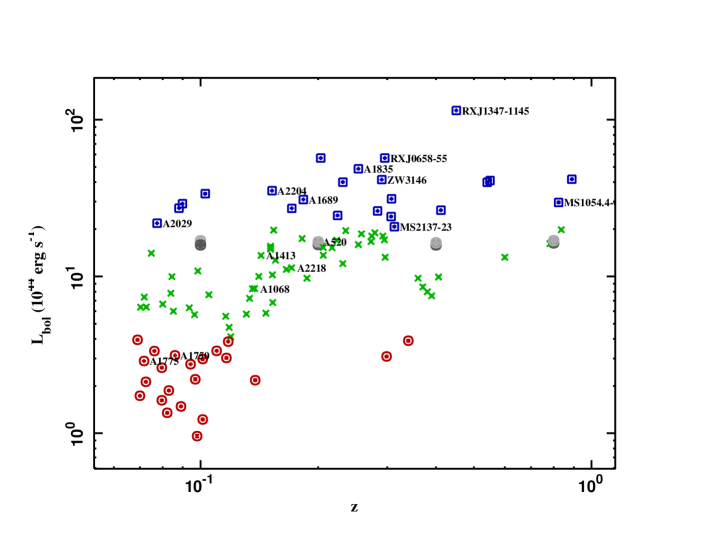The sample encompasses clusters with luminosities from $9\times 10^{43}~{}$erg s^-1 to $1.1\times 10^{46}~{}$erg s^-1, average temperatures from $2.2$ to $11.6~{}$keV (See Section 3.1) and redshifts from $z=0.069$ to $z=0.89$. The distribution of luminosities with redshift for the sample is shown in Figure 1 where the names of a subsample of well-known clusters are printed in the plot. Luminosities were calculated from the observed flux, using tabulated redshifts (as listed in NED), assuming a concordance cosmology (mentioned above), and applying a bolometric correction.

2.1. Data reduction

The data were reduced using standard pipeline processing and the calibration implementation as of XMM Science Analysis Software (SAS) version 6.5. Background flares from soft protons were removed using lightcurve filtering in both soft (MOS: 0.3-10 keV, PN: 0.3-12 keV) and hard (MOS: 10-12 keV, PN: 12-14 keV) X-ray bands. For the soft band, light curves were binned in 10 s intervals while we used 100 s bins for the hard band. In both cases the data were not included during the time when the count rate exceeded $3\sigma$ above the quiescent count rate, indicating a proton flare.

The event files were also filtered for non- X-ray events by selecting only single and double pixel events for PN and single to quadruple events for MOS. Bad pixels and pixel columns were removed by applying the standard keywords in event selection; FLAG=0 and #XMMEA_EM / #XMMEA_EP. The data reduction follows that described in Andersson et al. (2007).

Table 1Spectral fit parameters

Name	z	$T~{}$[keV]	Abundance wrt. Solar	$L_{bol}$ [erg s-1]	Exposure [ks]
CIZAJ1645.4-7334	0.069	$3.86^{+0.24}_{-0.22}$	$0.65^{+0.12}_{-0.11}$	$3.9~{}10^{44}$	14
A1837	0.070	$3.85^{+0.08}_{-0.08}$	$0.38^{+0.03}_{-0.03}$	$1.7~{}10^{44}$	45
A3112	0.070	$4.32^{+0.05}_{-0.04}$	$0.50^{+0.02}_{-0.02}$	$6.4~{}10^{44}$	21
A1775	0.072	$3.70^{+0.10}_{-0.06}$	$0.49^{+0.03}_{-0.03}$	$2.9~{}10^{44}$	23
A399	0.072	$6.92^{+0.23}_{-0.23}$	$0.28^{+0.04}_{-0.04}$	$7.4~{}10^{44}$	11
A1589	0.072	$4.81^{+0.20}_{-0.18}$	$0.30^{+0.06}_{-0.05}$	$2.1~{}10^{44}$	15
A2065	0.073	$5.36^{+0.11}_{-0.10}$	$0.27^{+0.02}_{-0.03}$	$6.4~{}10^{44}$	18
A401	0.075	$7.79^{+0.22}_{-0.23}$	$0.27^{+0.03}_{-0.03}$	$1.4~{}10^{45}$	11
A2670	0.076	$4.02^{+0.12}_{-0.11}$	$0.40^{+0.04}_{-0.04}$	$3.3~{}10^{44}$	17
A2029	0.077	$6.88^{+0.11}_{-0.08}$	$0.41^{+0.02}_{-0.02}$	$2.2~{}10^{45}$	11
RXCJ1236.7-3354	0.080	$2.80^{+0.11}_{-0.10}$	$0.46^{+0.08}_{-0.07}$	$1.6~{}10^{44}$	12
RXCJ2129.8-5048	0.080	$4.55^{+0.26}_{-0.19}$	$0.27^{+0.06}_{-0.06}$	$2.6~{}10^{44}$	21
A2255	0.080	$6.98^{+0.35}_{-0.28}$	$0.28^{+0.07}_{-0.05}$	$6.7~{}10^{44}$	10
RXCJ0821.8+0112	0.082	$3.69^{+0.29}_{-0.24}$	$0.28^{+0.10}_{-0.09}$	$1.3~{}10^{44}$	9
RXCJ1302.8-0230	0.083	$3.52^{+0.09}_{-0.09}$	$0.49^{+0.06}_{-0.05}$	$1.9~{}10^{44}$	22
A1650	0.084	$5.53^{+0.07}_{-0.08}$	$0.36^{+0.02}_{-0.02}$	$7.8~{}10^{44}$	37
A1651	0.084	$6.20^{+0.18}_{-0.16}$	$0.34^{+0.03}_{-0.03}$	$10.0~{}10^{44}$	10
A2597	0.085	$3.46^{+0.03}_{-0.03}$	$0.39^{+0.01}_{-0.01}$	$6.0~{}10^{44}$	56
A1750	0.086	$4.45^{+0.13}_{-0.13}$	$0.31^{+0.04}_{-0.04}$	$3.1~{}10^{44}$	29
A478	0.088	$6.04^{+0.04}_{-0.04}$	$0.37^{+0.01}_{-0.01}$	$2.7~{}10^{45}$	96
A278	0.089	$3.39^{+0.13}_{-0.14}$	$0.26^{+0.05}_{-0.05}$	$1.5~{}10^{44}$	27
A2142	0.090	$8.15^{+0.24}_{-0.28}$	$0.30^{+0.04}_{-0.04}$	$2.9~{}10^{45}$	6
A3921	0.094	$5.65^{+0.15}_{-0.14}$	$0.33^{+0.04}_{-0.04}$	$6.3~{}10^{44}$	29
A13	0.094	$5.00^{+0.17}_{-0.17}$	$0.27^{+0.04}_{-0.04}$	$2.8~{}10^{44}$	31
A3911	0.097	$5.94^{+0.19}_{-0.14}$	$0.26^{+0.03}_{-0.03}$	$5.7~{}10^{44}$	25
RXCJ2319.6-7313	0.097	$2.27^{+0.09}_{-0.07}$	$0.32^{+0.05}_{-0.05}$	$2.2~{}10^{44}$	8
CL0852+1618	0.098	$2.76^{+0.25}_{-0.21}$	$0.85^{+0.24}_{-0.19}$	$9.6~{}10^{43}$	31
A3827	0.098	$6.93^{+0.15}_{-0.13}$	$0.27^{+0.02}_{-0.02}$	$1.1~{}10^{45}$	21
RXCJ0211.4-4017	0.101	$2.22^{+0.07}_{-0.07}$	$0.43^{+0.07}_{-0.06}$	$1.2~{}10^{44}$	26
A2241	0.101	$3.66^{+0.45}_{-0.28}$	$0.81^{+0.26}_{-0.18}$	$3.0~{}10^{44}$	5
PKS0745-19	0.103	$6.44^{+0.07}_{-0.07}$	$0.34^{+0.01}_{-0.01}$	$3.4~{}10^{45}$	20
RXCJ0645.4-5413	0.105	$7.39^{+0.33}_{-0.26}$	$0.24^{+0.04}_{-0.04}$	$7.7~{}10^{44}$	13
RXCJ0049.4-2931	0.110	$4.02^{+0.19}_{-0.18}$	$0.40^{+0.07}_{-0.06}$	$3.4~{}10^{44}$	19
A1302	0.116	$6.59^{+0.46}_{-0.42}$	$0.53^{+0.10}_{-0.09}$	$5.6~{}10^{44}$	16
RXCJ0616.8-4748	0.116	$5.05^{+0.45}_{-0.44}$	$0.26^{+0.10}_{-0.10}$	$3.0~{}10^{44}$	9
RXCJ2149.1-3041	0.118	$3.53^{+0.07}_{-0.07}$	$0.47^{+0.04}_{-0.04}$	$3.8~{}10^{44}$	23
RXCJ1516.3+0005	0.118	$5.25^{+0.16}_{-0.15}$	$0.30^{+0.04}_{-0.04}$	$4.7~{}10^{44}$	25
RXCJ1141.4-1216	0.119	$3.53^{+0.06}_{-0.06}$	$0.53^{+0.04}_{-0.03}$	$4.1~{}10^{44}$	26
RXCJ0020.7-2542	0.131	$6.47^{+0.27}_{-0.23}$	$0.24^{+0.04}_{-0.04}$	$5.8~{}10^{44}$	16
RXCJ1044.5-0704	0.134	$3.67^{+0.04}_{-0.06}$	$0.36^{+0.03}_{-0.02}$	$7.3~{}10^{44}$	25
RXCJ0145.0-5300	0.136	$6.80^{+0.42}_{-0.44}$	$0.34^{+0.09}_{-0.08}$	$8.3~{}10^{44}$	14
A1068	0.138	$3.81^{+0.08}_{-0.07}$	$0.39^{+0.03}_{-0.03}$	$8.4~{}10^{44}$	20
RXJ1416.4+2315	0.138	$3.58^{+0.38}_{-0.33}$	$0.25^{+0.14}_{-0.13}$	$2.2~{}10^{44}$	6
RXCJ0605.8-3518	0.141	$4.52^{+0.08}_{-0.08}$	$0.39^{+0.03}_{-0.03}$	$1.0~{}10^{45}$	21
A1413	0.143	$7.30^{+0.19}_{-0.19}$	$0.36^{+0.04}_{-0.04}$	$1.4~{}10^{45}$	24
RXCJ2048.1-1750	0.147	$5.92^{+0.28}_{-0.23}$	$0.23^{+0.05}_{-0.05}$	$5.8~{}10^{44}$	23
A3888	0.151	$9.31^{+0.69}_{-0.51}$	$0.23^{+0.08}_{-0.07}$	$1.5~{}10^{45}$	5
A2034	0.151	$7.41^{+0.27}_{-0.21}$	$0.29^{+0.04}_{-0.04}$	$1.6~{}10^{45}$	12
RXCJ2234.5-3744	0.151	$7.88^{+0.22}_{-0.22}$	$0.19^{+0.03}_{-0.03}$	$1.5~{}10^{45}$	23
A2204	0.152	$6.44^{+0.08}_{-0.09}$	$0.37^{+0.02}_{-0.02}$	$3.5~{}10^{45}$	19
RXCJ0958.3-1103	0.153	$5.20^{+0.19}_{-0.20}$	$0.40^{+0.05}_{-0.05}$	$1.0~{}10^{45}$	8

Note. — Redshifts, temperatures, metal abundances (wrt. Solar), luminosities and exposure times for the sample. Redshifts are taken from the NED listing. Temperatures and metal abundances were derived using spectral fits (Section 3.1). Luminosities within a 1 Mpc aperture were derived using the SPI modeling (Section 3.2).

Table 2Spectral fit parameters, Contd.

Name	z	$T~{}$[keV]	Abundance wrt. Solar	$L_{bol}$ [erg s-1]	Exposure [ks]
A868	0.153	$5.86^{+0.54}_{-0.39}$	$0.21^{+0.08}_{-0.08}$	$6.8~{}10^{44}$	6
RXCJ2014.8-2430	0.154	$4.90^{+0.08}_{-0.07}$	$0.37^{+0.02}_{-0.02}$	$2.0~{}10^{45}$	23
A2104	0.155	$9.55^{+1.43}_{-0.97}$	$0.38^{+0.14}_{-0.13}$	$1.3~{}10^{45}$	5
RXCJ0547.6-3152	0.166	$6.92^{+0.22}_{-0.20}$	$0.31^{+0.04}_{-0.03}$	$1.1~{}10^{45}$	22
A2218	0.171	$7.17^{+0.21}_{-0.17}$	$0.22^{+0.03}_{-0.03}$	$1.1~{}10^{45}$	16
A1914	0.171	$9.49^{+0.28}_{-0.18}$	$0.25^{+0.03}_{-0.03}$	$2.7~{}10^{45}$	22
A665	0.182	$7.94^{+0.23}_{-0.24}$	$0.25^{+0.03}_{-0.03}$	$1.7~{}10^{45}$	57
A1689	0.183	$9.07^{+0.17}_{-0.12}$	$0.28^{+0.02}_{-0.02}$	$3.1~{}10^{45}$	35
A383	0.187	$4.21^{+0.09}_{-0.08}$	$0.46^{+0.04}_{-0.03}$	$9.7~{}10^{44}$	28
A520	0.199	$8.45^{+0.33}_{-0.26}$	$0.24^{+0.04}_{-0.03}$	$1.7~{}10^{45}$	38
A2163	0.203	$11.12^{+0.36}_{-0.39}$	$0.21^{+0.04}_{-0.04}$	$5.7~{}10^{45}$	10
A209	0.206	$7.21^{+0.27}_{-0.26}$	$0.27^{+0.04}_{-0.04}$	$1.5~{}10^{45}$	17
A963	0.206	$6.43^{+0.22}_{-0.19}$	$0.31^{+0.04}_{-0.03}$	$1.4~{}10^{45}$	23
A773	0.217	$7.41^{+0.33}_{-0.26}$	$0.29^{+0.05}_{-0.05}$	$1.5~{}10^{45}$	15
A1763	0.223	$7.67^{+0.34}_{-0.33}$	$0.34^{+0.05}_{-0.06}$	$1.7~{}10^{45}$	12
A2261	0.224	$8.66^{+0.71}_{-0.67}$	$0.41^{+0.11}_{-0.11}$	$2.5~{}10^{45}$	4
A267	0.231	$6.67^{+0.38}_{-0.37}$	$0.34^{+0.07}_{-0.06}$	$1.2~{}10^{45}$	15
A2390	0.231	$8.68^{+0.29}_{-0.27}$	$0.35^{+0.04}_{-0.04}$	$4.0~{}10^{45}$	12
RXJ2129.6+0005	0.235	$5.74^{+0.04}_{-0.10}$	$0.38^{+0.03}_{-0.03}$	$2.0~{}10^{45}$	43
A1835	0.253	$7.14^{+0.10}_{-0.11}$	$0.30^{+0.02}_{-0.02}$	$4.9~{}10^{45}$	37
RXCJ0307.0-2840	0.253	$6.47^{+0.38}_{-0.35}$	$0.32^{+0.06}_{-0.06}$	$1.6~{}10^{45}$	11
E1455+2232	0.258	$4.59^{+0.08}_{-0.09}$	$0.35^{+0.03}_{-0.03}$	$1.9~{}10^{45}$	33
RXCJ2337.6+0016	0.273	$7.74^{+0.66}_{-0.52}$	$0.19^{+0.07}_{-0.07}$	$1.7~{}10^{45}$	11
RXCJ0303.8-7752	0.274	$8.21^{+0.64}_{-0.62}$	$0.26^{+0.08}_{-0.07}$	$1.8~{}10^{45}$	10
A1758	0.279	$9.16^{+0.39}_{-0.43}$	$0.29^{+0.06}_{-0.06}$	$1.9~{}10^{45}$	44
RXCJ0232.2-4420	0.284	$7.13^{+0.31}_{-0.29}$	$0.30^{+0.05}_{-0.05}$	$2.6~{}10^{45}$	10
ZW3146	0.291	$6.21^{+0.14}_{-0.10}$	$0.33^{+0.02}_{-0.02}$	$4.1~{}10^{45}$	50
RXCJ0043.4-2037	0.292	$6.95^{+0.46}_{-0.42}$	$0.29^{+0.08}_{-0.07}$	$1.8~{}10^{45}$	10
RXCJ0516.7-5430	0.295	$8.33^{+0.84}_{-0.74}$	$0.19^{+0.09}_{-0.09}$	$1.7~{}10^{45}$	10
RXJ0658-55	0.296	$11.58^{+0.26}_{-0.35}$	$0.23^{+0.03}_{-0.03}$	$5.7~{}10^{45}$	29
RXCJ2308.3-0211	0.297	$7.22^{+0.91}_{-0.67}$	$0.40^{+0.12}_{-0.11}$	$1.3~{}10^{45}$	9
RXJ2237.0-1516	0.299	$3.46^{+0.44}_{-0.42}$	$0.46^{+0.24}_{-0.20}$	$3.1~{}10^{44}$	19
RXCJ1131.9-1955	0.307	$7.69^{+0.55}_{-0.40}$	$0.28^{+0.06}_{-0.06}$	$2.4~{}10^{45}$	11
RXCJ0014.3-3022	0.308	$8.36^{+0.46}_{-0.45}$	$0.24^{+0.05}_{-0.05}$	$3.1~{}10^{45}$	13
MS2137-23	0.313	$4.67^{+0.17}_{-0.19}$	$0.36^{+0.05}_{-0.06}$	$2.1~{}10^{45}$	11
MS1208.7+3928	0.340	$5.85^{+1.04}_{-0.80}$	$0.79^{+0.39}_{-0.33}$	$3.9~{}10^{44}$	11
RXJ0256.5+0006	0.360	$6.68^{+1.02}_{-0.80}$	$0.47^{+0.18}_{-0.17}$	$9.7~{}10^{44}$	11
RXJ0318.2-0301	0.370	$6.07^{+1.07}_{-0.81}$	$0.22^{+0.15}_{-0.15}$	$8.6~{}10^{44}$	16
RXJ0426.1+1655	0.380	$7.85^{+2.64}_{-1.73}$	$0.54^{+0.33}_{-0.27}$	$8.0~{}10^{44}$	10
RXJ1241.5+3250	0.390	$6.63^{+0.74}_{-0.72}$	$0.32^{+0.15}_{-0.14}$	$7.5~{}10^{44}$	17
A851	0.406	$6.25^{+0.41}_{-0.45}$	$0.22^{+0.07}_{-0.07}$	$9.9~{}10^{44}$	43
RXCJ2228+2037	0.412	$9.03^{+0.50}_{-0.49}$	$0.23^{+0.06}_{-0.06}$	$2.6~{}10^{45}$	23
RXJ1347-1145	0.451	$11.44^{+0.26}_{-0.29}$	$0.27^{+0.03}_{-0.03}$	$1.1~{}10^{46}$	32
CL0016+16	0.541	$9.20^{+0.50}_{-0.55}$	$0.29^{+0.06}_{-0.06}$	$4.0~{}10^{45}$	28
MS0451.6-0305	0.550	$10.02^{+0.80}_{-0.60}$	$0.36^{+0.08}_{-0.07}$	$4.1~{}10^{45}$	28
RXJ1120.1+4318	0.600	$6.09^{+0.89}_{-0.69}$	$0.54^{+0.18}_{-0.16}$	$1.3~{}10^{45}$	18
MS1137.5+6625	0.782	$8.58^{+2.33}_{-1.98}$	$0.35^{+0.37}_{-0.26}$	$1.6~{}10^{45}$	18
MS1054.4-0321	0.823	$9.20^{+1.26}_{-1.03}$	$0.22^{+0.13}_{-0.13}$	$3.0~{}10^{45}$	25
WARPJ0152.7-1357	0.837	$7.93^{+0.73}_{-0.45}$	$0.29^{+0.11}_{-0.11}$	$2.0~{}10^{45}$	48
CLJ1226.9+3332	0.890	$10.69^{+0.82}_{-0.81}$	$0.15^{+0.08}_{-0.08}$	$4.2~{}10^{45}$	69

Note. — Redshifts, temperatures, metal abundances (wrt. Solar), luminosities and exposure times for the sample. Redshifts are taken from the NED listing. Temperatures and metal abundances were derived using spectral fits (Section 3.1). Luminosities within a 1 Mpc aperture were derived using the SPI modeling (Section 3.2).

3. Data analysis methods

We analyze all objects using both simple spectral analysis, where a single spectrum is extracted and fitted, as well as the SPI analysis, using the Monte Carlo approach and modeling the clusters both spatially and spectrally.

3.1. Standard analysis

All clusters are first analyzed using “standard” spectral analysis. This was conducted by extracting X-ray counts from a circular region centered on the peak of X-ray emission. The extraction radius was determined by estimating the radius at which a circle encompasses 90% of the background subtracted surface intensity.

The background was estimated using the surface intensity at the edge of the field. Background spectra were extracted in regions outside the source extraction region. Point sources were detected using SAS routine emldetect using only sources measured with a likelihood above 100.

The extracted spectra were fitted using XSPEC (Arnaud, 1996) software, employing a MEKAL (Mewe et al., 1985, 1986; Kaastra, 1992; Liedahl et al., 1995) thermal plasma model with Solar abundances absorbed by a WABS (Morrison & McCammon, 1983) model, which we allow to be fitted as a free parameter. In the fit, the redshift was fixed to the known optical value as listed in the NED database entry.

The results of these “standard” spectral fits including plasma temperature and metal abundances w.r.t. Solar are listed in Table 1. The bolometric luminosities shown in the table are derived using the SPI analysis below. The redshift as given in NED is also shown as well as the average effective exposure time after filtering. All observations had usable data for all three EPIC detectors with the exception of A665, A1413, A2261, A2597 and A3921 where only the two MOS detectors were available.

3.2. SPI based MCMC analysis

The cluster event files are modeled using Smoothed Particle Inference (SPI) (Peterson, Marshall, & Andersson, 2007) with a Monte Carlo model of the XMM-Newton EPIC Camera (Andersson et al., 2007). Within the SPI analysis, clusters are modeled as conglomerations of 2D spatial Gaussians with individual spectral models. In this work we use the MEKAL model to describe the thermal plasma. Model photons are simulated and propagated through the detector model adding background Monte Carlo events representing internal fluorescent lines, electronic noise and soft proton signals. Data and model photons are binned in three dimensional adaptive bins and compared via a two-sample likelihood function. All parameters, spatial and spectral, are iterated in a Markov Chain with an adaptive step length. All model samples in the converged part of the chain are used to reconstruct the cluster.

3.2.1 SPI setup

The number of SPI particles are determined by the number of photons in the data so that, on average, $N_{\gamma}/N_{p}=400$, where $N_{p}$ is the number of particles and $N_{\gamma}$ is the number of X-ray events in the data. This number is chosen based on the Bayesian evidence calculation in Peterson, Marshall, & Andersson (2007) where we find the evidence reaching a plateau near 400 SPI particles for a 155000 photon observation. We choose to scale the number of particles with the number of photons since that is what ultimately determines the complexity of the data and we want a corresponding complexity of the model. We constrain the minimum number particles to be 100 and the maximum to be 1000.

The oversimulate factor, the factor that determines the number of model photons, is set so that there are 10 times as many photons in the model compared to the data with a maximum of 4 million model photons. This number is motivated by the drastic improvement of the optimization when using a factor of 10 or above as shown in Peterson, Marshall, & Andersson (2007). The upper limit is set to minimize computing time for very well exposed clusters.

The three dimensional (x,y,pulseheight) adaptive binning grid is created so that every bin with more than 20 photons is divided in 2. The spectral dimension is divided 10 times more often than the spatial dimensions on average in order to achieve appropriate spectral resolution.

3.2.2 Model setup

The setup of the instrumental background model, consisting of electronic noise, soft proton detections and fluorescent emission lines, is analogous to the setup in Andersson et al. (2007). The fraction of photons going to the background model is variable from 0 to 1, as are the relative normalizations of the included components.

We model the soft X-ray background originating from our Galaxy using a uniform emission component consisting of a thermal plasma spectral model. This emission consists of local (and thus weakly absorbed) component plus an absorbed, more distant contribution from the Galactic halo; it is adequately described as several thermal components in the 0.05-0.5 keV range (e.g.  Kuntz & Snowden, 2000). Motivated by our analysis of blank sky data files, we find that unabsorbed MEKAL model at temperature of 0.16 keV, with metal abundance of $0.3Z_{\sun}$ at $z=0$ describes the data well, and this is a model we adopt for the Galactic background: given the limited EPIC bandpass, our approximation is sufficient. We keep in mind that the spectral accuracy of the method is limited in the regions of the clusters where a large fraction of the photons come from the X-ray background, such as at large radii. While there the cluster flux is low, the adaptive binning grid will allow only gross spectral features to be detectable.

Similarly the Cosmic X-ray Background (CXB) - presumably due to superposition of unresolved AGN - is modeled using a powerlaw with photon index $\Gamma=1.47$ and absorption fixed at the galactic value at the coordinates as given by Dickey & Lockman (1990).

The cluster model consists of spatial Gaussians described by an x and y position and a Gaussian $\sigma$. Each Gaussian is assigned a spectral MEKAL model with WABS absorption. The allowed ranges for the absorbing equivalent hydrogen column, $n_{H}$, the plasma temperature, $T$, the metallicity w.r.t. the Solar values of Anders & Grevesse (1989), $Z$, and redshift $z$ are shown in Table 3. Absorption is assumed to be within 20% of the $n_{H,gal}$ values of Dickey & Lockman (1990) at the cluster coordinates.

Table 3Cluster model parameter ranges used in the SPI analysis

Parameter	min value	max value
Spectral model
$n_{H}$	0.8$~{}n_{H,gal}$	1.2$~{}n_{H,gal}$
$T$ [keV]	$0.5$	$15.0$
$Z$ wrt. Solar	0	2
$z$	$z_{NED}$ fixed
Spatial model
$x$	$-12\arcmin$	$+12\arcmin$
$y$	$-12\arcmin$	$+12\arcmin$
ln$~{}\sigma(\arcsec)$	0	6

Note. — The parameter ranges used in the SPI modeling. $n_{H}$ is variable within 20 % of the values of Dickey & Lockman (1990). The $x$ and $y$ positions are variable within $12\arcmin$ of the XMM nominal pointing.

3.2.3 Convergence

In Peterson, Marshall, & Andersson (2007) a criterion for convergence of the Markov chain is applied and it is found to converge within 200 iterations. Here, the more conservative limit of 750 iterations is used as the point of convergence. All the results derived from the model samples are from the iterations from 750 to 2000. This range is chosen based on slight deviations in cluster properties when derived from iteration 200 and onward.

3.2.4 Simulated clusters

In order to study the systematic effects induced by the X-ray mirror PSF and limited statistics on faint sources, we simulate a massive, spherically symmetric, weak cooling core cluster at $z=0.1$, $0.2$, $0.4$ and $0.8$. The simulated cluster model consists of two superimposed beta models with core radii of $74$ and $370$ kpc, both with $\beta=0.7$. The smaller, core component is assigned a spectral model with $kT=4~{}$keV whereas the ambient component has $kT=9~{}$keV. The normalization ratio of the cold to the hot component in terms of emission measure, $\int n_{e}n_{p}\mathrm{d}V$, is $11/9$ and the overall normalization is set so that the total bolometric luminosity of the cluster is $L_{Bol}=1.7~{}10^{45}~{}$erg s^-1, a typical luminosity in our sample, present at all redshifts $0.1\leq z<0.8$. The model is based on observations of the cool core clusters A2029 and A2241. Bolometric luminosities for the cluster sample are estimated using the $0.01$ - $100~{}$ keV energy band as described in Section 4.1.

These simulated clusters all have the same background level ($5~{}10^{-3}$ s${}^{-1}~{}(\arcmin)^{-2}$) and are assumed to have an effective exposure time of 20 ks in all 3 EPIC detectors. The assumed luminosity results in a total number of 850058, 209294, 46358 and 9353 cluster photons respectively for the $z=0.1$, $0.2$, $0.4$ and $0.8$ clusters in the adopted energy range (MOS:0.3-10 keV, pn:1.1-10 keV). As a reference, the same clusters are also simulated without background and reconstructed separately.

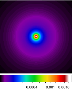
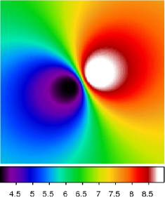
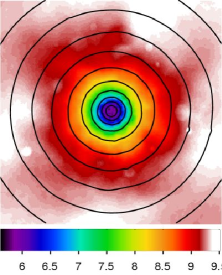
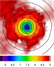
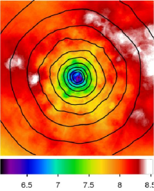
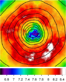
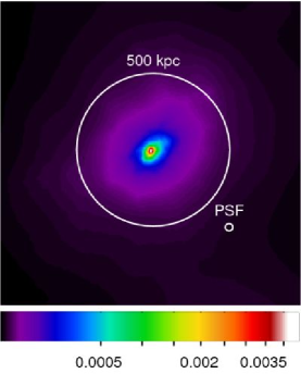
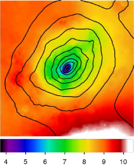
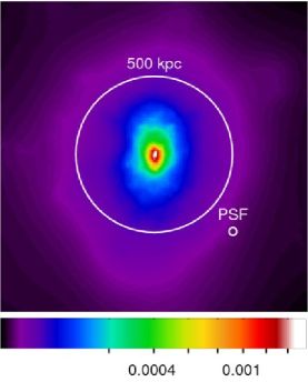
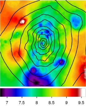
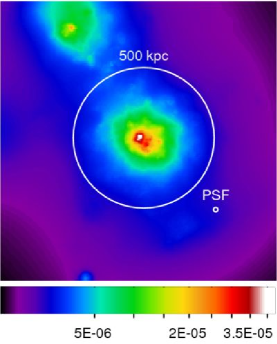
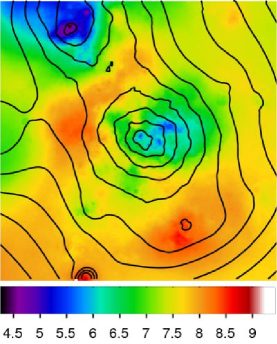
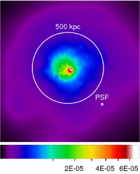
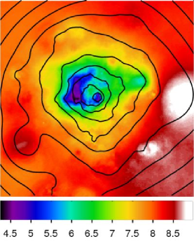
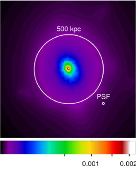
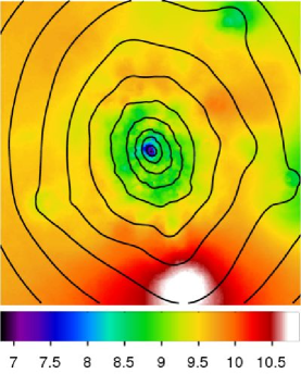
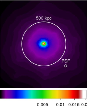
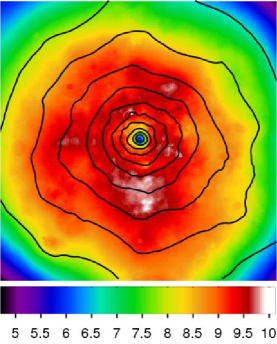
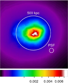
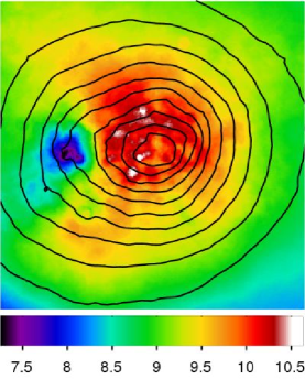
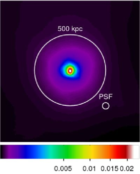
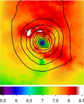
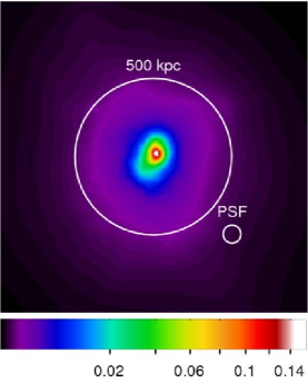
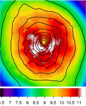
The apparent evolution with $z$ in the derived properties for these identical clusters will be used to categorize the clusters in the sample. Figure 2 shows the original cluster model before propagated through the instrument model visualized with a luminosity and temperature map within the 1 Mpc radius. Luminosity per unit solid angle in this Figure is given in units of $10^{44}~{}$erg s^-1 $(\arcsec)^{-2}$ and temperature in keV.

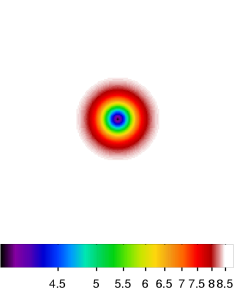
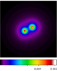
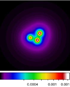
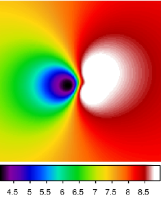
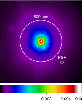
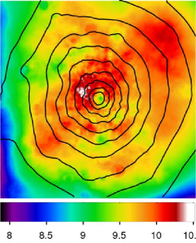
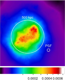
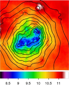
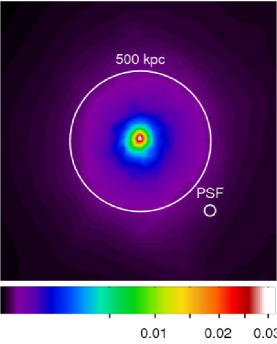
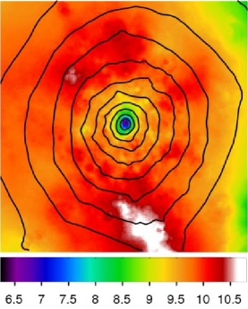
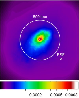
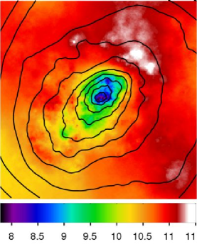
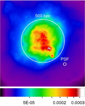
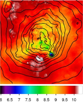
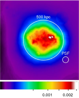
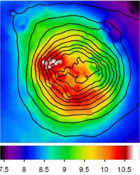
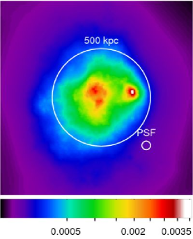
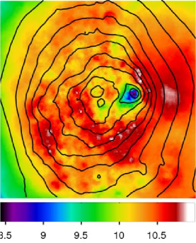
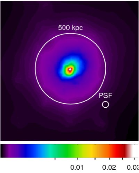
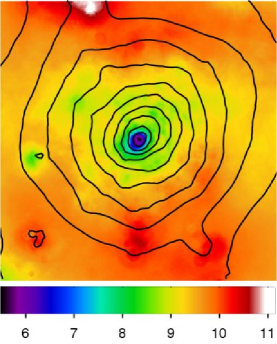
In order to follow the evolution of substructure in clusters we also simulate two sets of clusters with irregular morphology, one using a two “subcluster” model and the other, a three “subcluster” model. The two-subcluster model consists of two beta models, at 4 and 9 keV respectively, each with $r_{c}=74~{}$kpc and $\beta=0.7$ separated by $300~{}$kpc. The total luminosity of the clusters is the same as for the original cool core cluster, $L_{Bol}=1.7~{}10^{45}~{}$erg s^-1. The cluster model is shown in Figure 3. The three-subcluster model consists of three beta models, at 4, 9 and 9 keV respectively, with core radii of $r_{c}=74~{}$kpc and $\beta=0.7$. The clusters are separated by a triangle with sides of $300$, $200$ and $200~{}$kpc. The total luminosity of the three clusters is $L_{Bol}=1.7~{}10^{45}~{}$erg s^-1. This model is shown in Figure 4.

Figure 2.— $2\times 2$ Mpc images of the bolometric luminosity in units of $10^{44}~{}$erg s^-1 $(\arcsec)^{-2}$ (left panel) and temperature in keV (right panel) of the original simulated cool core cluster model.

Figure 3.— $2\times 2$ Mpc images of the bolometric luminosity in units of $10^{44}~{}$erg s^-1 $(\arcsec)^{-2}$ (left panel) and temperature in keV (right panel) of the simulated two-subcluster model.

Figure 4.— $2\times 2$ Mpc images of the bolometric luminosity in units of $10^{44}~{}$erg s^-1 $(\arcsec)^{-2}$ (left panel) and temperature in keV (right panel) of the simulated three-subcluster model.

4. Post-processing

Here, we describe the raw output of the SPI analysis - temperature and luminosity maps of the clusters considered here - and discuss the estimation of uncertainties. We also outline the methods that will be applied in the subsequent sections towards determination of the luminosity and temperature structure of clusters in our sample. First, we consider a luminosity and temperature contrast analysis with the primary goal to identify clusters containing cool cores. The luminosity contrast analysis is similar to that of Vikhlinin et al. (2006b). We also consider the “Power Ratios” method, suggested by Buote & Tsai (1995) to quantify the cluster substructuring. Finally, we propose a new method, the “Temperature two-point correlation” which is specifically designed to quantify the temperature structure, and is enabled by the SPI analysis.

4.1. Temperature and luminosity maps

We create $2\times 2~{}$Mpc cluster luminosity and emission weighted temperature maps centered on the peak of cluster emission with $10~{}$kpc bins. The method of creating median parameter maps is described in Andersson et al. (2007). Maps are created for each sample in the chain from iteration 750 to 2000 and are averaged by taking the median in each spatial point over the whole sample.

Point sources are removed by filtering out all cluster particles within a radius of $-16.1+\log_{10}(L_{2})~{}15~{}\arcsec$, from the point source as detected by emldetect, where $L_{2}$ is the likelihood of detection. We find that this method successfully removes any point source contamination without removing the cluster flux in the region of the point source. This method is effective because particles that represent the point source emission are generally smaller in size whereas the cluster particles are larger and fill the region where the point source was removed. 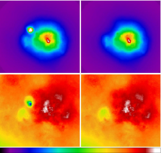An example of such point source removal is shown in Figure 5 which shows maps of luminosity (top) and temperature (bottom) for Abell 3888 before (left) and after (right) point source removal.

Figure 5.— $10\arcmin\times 10\arcmin$ field showing luminosity (top) and temperature (bottom) maps of Abell 3888 before (left) and after (right) point source removal. The color scale in the luminosity map is set so that white corresponds to the maximum cluster flux. The point source is 100 times brighter than this level. The scale in the temperature map ranges from 2 to 10 keV.

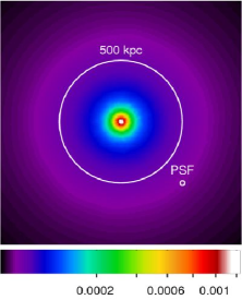
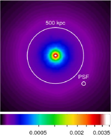
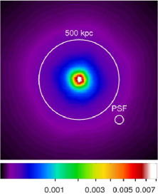
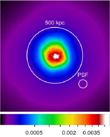
The reconstruction of the four simulated cool core clusters within $2~{}\times~{}2~{}$Mpc is shown in Figure 6 where luminosity per unit solid angle is given in units of $10^{44}~{}$erg s^-1 $(\arcsec)^{-2}$ and temperature in units of keV. Here, the effects of the XMM point spread function (PSF) as well as the loss of photons with redshift is clearly seen as a distortion and flattening of the profile at high $z$.

Figure 6.— Luminosity (top) and temperature (bottom) maps for the reconstructed simulated cool core clusters, with background, at redshift 0.1, 0.2, 0.4 and 0.8. Luminosity per unit solid angle is in units of $10^{44}~{}$erg s^-1 $(\arcsec)^{-2}$ and temperatures in keV.

The maps for a subsample of clusters are shown in Figures 16 through 32 including the named clusters in Figure 1. We comment briefly on these maps in Section 5.4 and compare them to previously published results. Note that the temperatures in Table 1 do not necessarily agree with the scale shown in the figures. This is because these values are derived using two different methods. The tabulated values are determined using standard analysis (Section 3.1) requiring a single value of gas temperature for the whole cluster, whereas the parameter maps are created using a range of temperatures derived from the SPI runs (Section 3.2). The source of the disagreement has to do with the fact that SPI bases the spectral modeling on superpositions of thermal spectra with many different temperatures. The fact that the similarities between these spectra increase with higher temperature implies that the average temperature value of these also increases. It also becomes dependent on the prior range of temperatures (here: 0.5 - 15 keV). Whenever referring to the cluster average temperature, the tabulated values are used. A bolometric correction is applied to the cluster particles individually, where the temperature, abundance and emission measure of the particle are used to calculate a bolometric luminosity in the 0.01 eV to 100 keV range using the MEKAL spectral model. This is the luminosity that is listed in Table 1.

4.2. Estimation of uncertainties

In all cases, except for the temperature and elemental abundance values used in Table 1, uncertainties are estimated by identifying 5 independent sets of samples in the Markov chain posterior. The samples are taken sequentially in ranges containing 250 iterations each, starting at iteration 750. The luminosity and temperature maps and the quantities derived from these are then evaluated separately and the uncertainty on these quantities is determined from the rms scatter within these 5 sets. This is a valid approximation of statistical uncertainty because each subset can be seen as an independent reconstruction of the cluster. The motions of particles in the parameter space are large and within a few iterations there is no memory about earlier states. This is largely due to the high dimensionality of the overall parameter space and the lack of local likelihood maxima. Of course, it would be more accurate to use more than 5 sets for this calculation but at least 250 iterations are needed in order to describe a cluster model and there is a limitation in CPU time to produce more iterations.

4.3. Luminosity and temperature contrast methods and identification of cooling clusters

A common definition of a “cooling flow” cluster regards the central cooling time, $t_{cool}=T/\mathrm{d}(ln(T))$, being much less than a “Hubble time”, $t_{cool}<<t_{H}$. The calculation of the cooling time requires high resolution spatially resolved spectroscopy which is not available for most of the clusters in our sample. Instead we use the information about the steepness of the luminosity profile as well as the gradient of temperature in the cluster core to empirically select the clusters with cool cores.

The luminosity contrast is calculated as

$$C_{L}=\frac{L\left(r\leq 0.02r_{500}\right)}{L\left(0.08r_{500}\leq r<0.12r_{500}\right)}$$ (1)

where $L$ is luminosity per solid angle. We use the luminosity based definition of $r_{500}$;

$$r_{500}=909~{}E(z)~{}\left(\frac{L_{bol}}{10^{44}\mathrm{erg~{}s}^{-1}}\right)^{0.172}\mathrm{kpc}.$$ (2)

where

$$E(z)=H(z)/H_{0}=$$

$$\sqrt{(1+z)^{2}~{}(1+\Omega_{M}~{}z)-z~{}(2+z)~{}\Omega_{\Lambda}}.$$ (3)

This value of $r_{500}$ is derived by combining the $M$-$T$ relation from Arnaud et al. (2005) and the $L$-$T$ relation from Arnaud & Evrard (1999). The fractions of $r_{500}$ are used to account for the difference in size for clusters of various luminosities.

Similarly we define the temperature contrast as

$$C_{T}=\frac{T\left(r\leq 0.02r_{500}\right)}{T\left(0.45r_{500}\leq r<0.55r_{500}\right)}$$ (4)

where we choose to estimate the gradient farther from the core ($0.5r_{500}$) than for the luminosity contrast above because it is less sensitive to smearing by redshift dependent effects. We find that the radius of $0.5r_{500}$ is where we could get the most distinguishing power. We discuss the use of $C_{L}$ and $C_{T}$ towards identifying cooling clusters in Section 5.1.

4.4. Power Ratios method

One of the successful approaches towards assessing the amount of substructure in clusters is the power ratios method (Buote & Tsai, 1995). It was used in Jeltema et al. (2005) for a sample of Chandra-observed clusters to establish that clusters are more dynamically active at high $z$. This method is based on the multipole expansion of the surface brightness $\Sigma(R,\phi)$ around the cluster centroid where the multipole moments $a_{m}$ and $b_{m}$ are

$$a_{m}(R)=\int_{R^{\prime}\leq R}\Sigma(R,\phi)(R^{\prime})^{m}\cos m\phi^{\prime}\mathrm{d}^{2}x^{\prime}$$ (5)

$$b_{m}(R)=\int_{R^{\prime}\leq R}\Sigma(R,\phi)(R^{\prime})^{m}\sin m\phi^{\prime}\mathrm{d}^{2}x^{\prime}$$ (6)

so that the powers in the multipole $m$ can be written

$$P_{0}=\left(a_{0}\mathrm{ln}(R)\right)^{2}$$ (7)

$$P_{m}=\frac{1}{2m^{2}R^{2m}}\left(a^{2}_{m}+b^{2}_{m}\right).$$ (8)

Here, we define the location of the cluster centroid by the requirement that $P_{1}$ should be zero at this location. The above method is applied to the luminosity maps described in the previous section and the ratios $P_{2}/P_{0}$ and $P_{3}/P_{0}$ are calculated within a radius of 500 kpc. We expect that $P_{2}/P_{0}$ will be larger for elongated clusters whereas $P_{3}/P_{0}$ will be large for clusters with much substructure in the luminosity map.

4.5. Temperature two-point correlation

We suggest that the variation of temperature inside the clusters can be estimated and characterized by taking a (non-standard) two point correlation of the temperature difference, weighted by products of luminosity so as to enhance temperature differences among the regions with the highest brightness. This is accomplished by taking the following sum over all 10 kpc $\times$ 10 kpc pixels in the generated maps:

$$A(r_{k})=\sqrt{\sum^{i,j}\sqrt{L_{i}~{}L_{j}}~{}(T_{i}-T_{j})^{2}/L_{T}}\\$$ (9)

where $L_{i}$ is the luminosity of pixel $i$, $T_{i}$ is the temperature and $L_{T}=\sum^{i,j}\sqrt{L_{i}~{}L_{j}}$. $i$ and $j$ are such that both $(x_{i},y_{i})$ and $(x_{j},y_{j})$ cover all points within 500 kpc of the centroid calculated in Section 4.4. $A$ is binned based on the distance between $i$ and $j$ as $10k~{}$kpc$<r_{k}\leq 10(k+1)~{}$kpc, $k=0\ldots 99$, where $r_{k}=\sqrt{(x_{i}-x_{j})^{2}+(y_{i}-y_{j})^{2}}$ is the pixel distance and $(x_{i},y_{i})$ is the spatial position of pixel $i$.

This statistic is designed to quantify the amount of distortion in the intra cluster medium, specifically regarding temperature features that can result from cluster mergers. Basically, it gives a “power spectrum” of strong temperature gradients over different scales, where the “strength” of the gradient is determined by $\sqrt{L_{i}~{}L_{j}}$. In integrating this quantity over small or large distances it should be possible to distinguish small scale features, such as cooling cores, from larger scale disturbances. We discuss the application of this method in Section 5.3.1.

5. Results

5.1. Identification of cooling core clusters

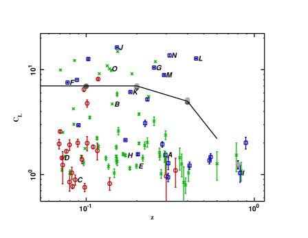
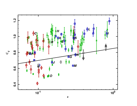
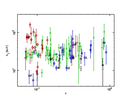
The first step is to identify clusters with cooling cores. We use the approach described in Section 4.3, and plot the luminosity contrast vs redshift in Figure 7 (left panel). Here, we also show the names for some well known clusters. Low $L_{X}$ clusters ($<4~{}10^{44}~{}$erg s^-1) are shown as red circles, intermediate $L_{X}$ clusters ($4~{}10^{44}~{}$erg s${}^{-1}\leq L_{X}<2~{}10^{45}~{}$erg s^-1) as green stars and high $L_{X}$ clusters ($\geq 2~{}10^{45}~{}$erg s^-1) as blue squares. Likewise, the temperature contrast vs redshift is shown in Figure 7 (right panel).

In Figure 7 we also show the calculated values for our simulated cool core cluster at redshift $z=0.1$, $0.2$, $0.4$ and $0.8$. It is easily seen that the effects of PSF smoothing and loss of photons due to increased distance severely affects both quantities. We show both the simulated clusters with (dark gray) and without (light gray) simulated background, totaling 8 simulated clusters.

$C_{L}$ is estimated at $0.1~{}r_{500}$ ($\sim 10^{\prime\prime}$ at $z=0.8$) and it becomes increasingly difficult to estimate at high redshifts. This can be seen in the sharp drop in $C_{L}$ in the trend of the simulated clusters above $z=0.4$. At $z=0.8$, the detection of cooling cores using $C_{L}$ is no longer sensitive and thus we decide to rely on the $C_{T}$ statistic alone for identification purposes above $z=0.6$. We identify those clusters with a $C_{L}$ above a line interpolated between the points set by the simulated clusters as cool core clusters. This cut corresponds to a linear interpolation of the points $C_{L}=(7,7,5,2.2)$ at $z=(0.1,0.2,0.4,0.6)$. This comfortably separates known cool core clusters (e.g. A2029) from disturbed and intermediate core clusters (e.g. A1689).

For $C_{T}$, the simulated clusters can be seen to have a trend that is more linear and not as dramatic as the trend in $C_{L}$. This is largely due to the larger radius ($0.5~{}r_{500}$) used when calculating $C_{T}$. Using $C_{T}$ to identify cool core clusters we make a cut corresponding to a straight line approximately following the trend of the simulated clusters so that clusters below the line, $C_{T}\leq 0.85+0.15~{}\log{z}$, are selected. These cuts select well known cooling clusters like A1068, A1835 and A2204 but fail to select clusters that are known not to have pronounced cool cores such as A1689 and A1413.

In subsequent plots we show the values for the reconstructions of the simulated clusters as filled circles and use this to measure how accurately a weak cooling core cluster at different redshifts can be resolved. The cuts are shown in Figure 7.

Figure 7.— Luminosity contrast (left) and temperature contrast (right) as a function of redshift. The different symbols represent luminosity (red circles $\geq 10^{43}~{}$erg s^-1, green stars $\geq 4~{}10^{44}~{}$erg s^-1, and blue squares $\geq 2~{}10^{45}~{}$erg s^-1). The cuts on $C_{L}$ and $C_{T}$ are shown as solid lines. The cooling clusters are above and below the line respectively. The simulated cool core clusters without (with) background are shown as light (dark) gray filled circles, occasionally overlapping. A few selected clusters are denoted using letters from A to O as follows: (A) RXJ0658-55, (B) A1413, (C) A1750, (D) A1775, (E) A520, (F) A2029, (G) A1835, (H) A2218, (I) MS1054.4-0321, (J) A2204, (K) A1689, (L) RXJ1347-1145, (M) ZW3146, (N) MS2137-23, (O) A1068.

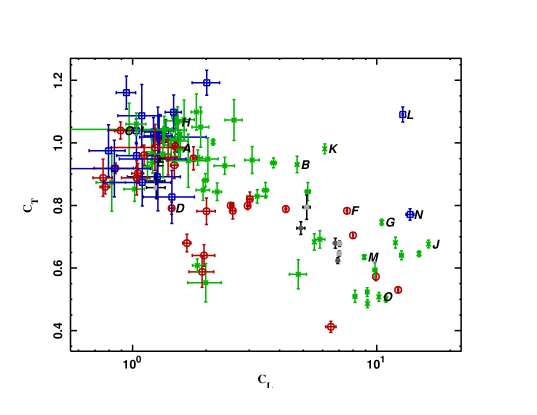
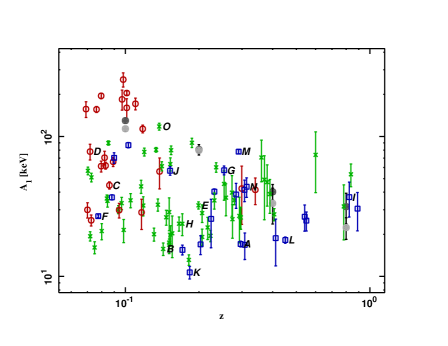
In Figure 8 we also show $C_{T}$ plotted against $C_{L}$, clearly showing the separation of cooling clusters like A1835 and A2204 (G, J - shown bottom right), nearly isothermal clusters such as A1413 and A1689 (B, K - shown center) and disturbed clusters like A2218 and A520 (H, E - shown top left).

Figure 8.— Temperature contrast plotted versus luminosity contrast. Here the different symbols represent redshift (red circles $0.069\leq z<0.1$, green stars $0.1\leq z<0.3$, and blue squares $z\geq 0.3$). Simulated cool core clusters are shown as filled gray circles. Letters from A to O denote a few selected clusters (see Figure 7).

Out of 101 clusters, 31 are identified as cooling clusters.

5.2. Dynamical activity

5.2.1 Power ratios

Table 4Power ratios

Name	$P_{2}/P_{0}(\times 10^{-7})$	$P_{3}/P_{0}(\times 10^{-7})$
CIZAJ1645.4-7334	$4.72\pm 0.95$	$0.41\pm 0.49$
A1837	$112\pm 7$	$2.37\pm 0.31$
A3112	$39.5\pm 1.6$	$0.085\pm 0.031$
A1775	$0.5\pm 0.33$	$3.86\pm 0.65$
A399	$62.0\pm 3.2$	$3.55\pm 0.31$
A1589	$298\pm 17$	$0.88\pm 0.51$
A2065	$208\pm 6$	$0.089\pm 0.032$
A401	$104\pm 3$	$0.92\pm 0.07$
A2670	$4.96\pm 0.91$	$4.07\pm 0.43$
A2029	$55.9\pm 2.1$	$0.051\pm 0.022$
RXCJ1236.7-3354	$21.6\pm 8.6$	$8.97\pm 2.72$
RXCJ2129.8-5048	$78.0\pm 7.8$	$27.1\pm 1.8$
A2255	$64.5\pm 5.0$	$0.58\pm 0.42$
RXCJ0821.8+0112	$106\pm 16$	$0.87\pm 0.58$
RXCJ1302.8-0230	$45.0\pm 11.7$	$0.59\pm 0.63$
A1650	$87.9\pm 2.3$	$0.24\pm 0.06$
A1651	$35.6\pm 3.1$	$0.12\pm 0.08$
A2597	$26.5\pm 0.6$	$0.058\pm 0.026$
A1750	$39.9\pm 5.7$	$1.84\pm 0.73$
A478	$46.4\pm 0.5$	$0.054\pm 0.004$
A278	$16.2\pm 2.1$	$1.23\pm 0.57$
A2142	$247\pm 9$	$0.15\pm 0.05$
A3921	$228\pm 10$	$2.2\pm 0.48$
A13	$88.2\pm 10.1$	$0.19\pm 0.12$
A3911	$344\pm 11$	$2.45\pm 0.51$
RXCJ2319.6-7313	$128\pm 18$	$0.22\pm 0.09$
CL0852+1618	$12.5\pm 9.6$	$22.9\pm 6.5$
A3827	$17.0\pm 1.7$	$0.96\pm 0.15$
RXCJ0211.4-4017	$18.3\pm 1.2$	$1.48\pm 0.55$
A2241	$7.01\pm 1.39$	$0.48\pm 0.36$
PKS0745-19	$36.0\pm 1.7$	$0.018\pm 0.01$
RXCJ0645.4-5413	$126\pm 6$	$2.11\pm 0.67$
RXCJ0049.4-2931	$13.3\pm 2.3$	$0.19\pm 0.14$
A1302	$28.9\pm 3.0$	$0.26\pm 0.23$
RXCJ0616.8-4748	$112\pm 18$	$3.0\pm 1.7$
RXCJ2149.1-3041	$29.3\pm 3.7$	$0.028\pm 0.015$
RXCJ1516.3+0005	$82.9\pm 4.0$	$0.63\pm 0.41$
RXCJ1141.4-1216	$19.4\pm 1.5$	$0.12\pm 0.11$
RXCJ0020.7-2542	$118\pm 6$	$1.36\pm 0.31$
RXCJ1044.5-0704	$47.0\pm 3.0$	$0.77\pm 0.09$
RXCJ0145.0-5300	$342\pm 29$	$2.63\pm 0.93$
A1068	$63.0\pm 4.4$	$1.21\pm 0.32$
RXJ1416.4+2315	$180\pm 20$	$3.37\pm 3.16$
RXCJ0605.8-3518	$47.0\pm 3.0$	$0.52\pm 0.17$
A1413	$192\pm 3$	$0.19\pm 0.1$
RXCJ2048.1-1750	$34.4\pm 4.4$	$3.92\pm 0.34$
A3888	$117\pm 7$	$6.33\pm 0.8$
RXCJ2234.5-3744	$119\pm 4$	$4.06\pm 0.49$
A2034	$84.5\pm 8.4$	$0.41\pm 0.21$
A2204	$3.81\pm 0.33$	$0.077\pm 0.045$
RXCJ0958.3-1103	$79.0\pm 9.1$	$0.14\pm 0.12$

Note. — Results of the Power Ratio analysis (Section 4.4) of the clusters.

Table 5Power ratios

Name	$P_{2}/P_{0}(\times 10^{-7})$	$P_{3}/P_{0}(\times 10^{-7})$
A868	$105\pm 6$	$0.92\pm 0.98$
RXCJ2014.8-2430	$15.8\pm 1.2$	$0.37\pm 0.13$
A2104	$68.0\pm 16.7$	$2.83\pm 2.54$
RXCJ0547.6-3152	$29.4\pm 3.1$	$0.33\pm 0.14$
A2218	$72.8\pm 5.6$	$1.14\pm 0.36$
A1914	$32.4\pm 1.0$	$2.45\pm 0.26$
A665	$44.8\pm 3.5$	$7.75\pm 0.77$
A1689	$27.6\pm 2.0$	$0.64\pm 0.12$
A383	$1.63\pm 0.26$	$0.62\pm 0.17$
A520	$65.3\pm 11.2$	$3.87\pm 0.46$
A2163	$45.6\pm 5.9$	$10.7\pm 1.7$
A209	$98.8\pm 5.5$	$1.18\pm 0.83$
A963	$8.14\pm 1.32$	$1.34\pm 0.67$
A773	$83.2\pm 11.2$	$0.82\pm 0.39$
A1763	$218\pm 8$	$1.36\pm 1.3$
A2261	$12.9\pm 11.4$	$2.79\pm 1.7$
A267	$95.8\pm 9.2$	$0.92\pm 0.64$
A2390	$149\pm 7$	$2.97\pm 0.86$
RXJ2129.6+0005	$66.1\pm 1.4$	$0.21\pm 0.03$
A1835	$10.2\pm 0.4$	$0.36\pm 0.09$
RXCJ0307.0-2840	$14.6\pm 3.8$	$2.23\pm 0.51$
E1455+2232	$16.1\pm 0.9$	$0.12\pm 0.08$
RXCJ2337.6+0016	$282\pm 29$	$1.16\pm 0.42$
RXCJ0303.8-7752	$37.4\pm 13.7$	$2.01\pm 0.87$
A1758	$502\pm 13$	$0.78\pm 0.32$
RXCJ0232.2-4420	$50.6\pm 4.8$	$2.5\pm 0.62$
ZW3146	$11.6\pm 1.3$	$0.37\pm 0.08$
RXCJ0043.4-2037	$58.5\pm 12.9$	$2.31\pm 2.39$
RXCJ0516.7-5430	$296\pm 54$	$8.28\pm 5.55$
RXJ0658-55	$116\pm 3$	$8.73\pm 0.95$
RXCJ2308.3-0211	$23.3\pm 4.2$	$1.44\pm 0.74$
RXJ2237.0-1516	$198\pm 41$	$8.29\pm 7.19$
RXCJ1131.9-1955	$142\pm 18$	$2.03\pm 1.29$
RXCJ0014.3-3022	$5.54\pm 4.01$	$7.16\pm 1.1$
MS2137-23	$1.47\pm 0.96$	$0.37\pm 0.49$
MS1208.7+3928	$322\pm 293$	$23.4\pm 26.9$
RXJ0256.5+0006	$6.12\pm 2.42$	$64.0\pm 15.3$
RXJ0318.2-0301	$39.7\pm 20.2$	$4.11\pm 3.27$
RXJ0426.1+1655	$35.9\pm 37.5$	$4.66\pm 5.68$
RXJ1241.5+3250	$27.4\pm 17.9$	$12.6\pm 9.9$
A851	$304\pm 30$	$6.49\pm 2.24$
RXCJ2228+2037	$144\pm 27$	$8.23\pm 3.18$
RXJ1347-1145	$32.6\pm 1.0$	$0.87\pm 0.24$
CL0016+16	$114\pm 17$	$5.54\pm 2.87$
MS0451.6-0305	$82.3\pm 5.1$	$7.01\pm 2.19$
RXJ1120.1+4318	$137\pm 49$	$9.82\pm 7.75$
MS1137.5+6625	$11.5\pm 11.9$	$10.5\pm 7.8$
MS1054.4-0321	$220\pm 73$	$17.3\pm 14.6$
WARPJ0152.7-1357	$2880\pm 260$	$27.6\pm 19.4$
CLJ1226.9+3332	$11.1\pm 3.2$	$0.87\pm 0.4$

Note. — Results of the Power Ratio analysis (Section 4.4) of the clusters.

In assessing the dynamical activity in the clusters in our sample we perform a multipole expansion of our luminosity maps as described in Section 4.4. The power ratios $P_{2}/P_{0}$ and $P_{3}/P_{0}$ are calculated to a radius of 500 kpc in order to quantify the amount of substructure in the sample. These are listed in Table 4.

Here we divide the sample in 3 redshift bins; a local $z$ bin ($z<0.1$), a low-$z$ bin ($0.1\leq z<0.3$) and a high-$z$ bin ($z>0.3$). The results of the multipole expansion are shown in Table 6 where we show the average values of $P_{2}/P_{0}$ and $P_{3}/P_{0}$ for the 3 samples. We also show the result obtained when using only the cooling core clusters identified in previous sections. These are not excluded from the other samples.

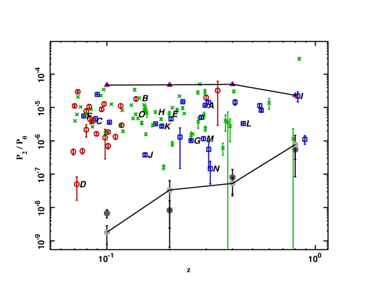
The values of $P_{2}/P_{0}$ and $P_{3}/P_{0}$ are plotted against $z$ in Figures 9 and 10 respectively where the simulated cool core clusters are shown as filled circles connected by black lines. In Figure 9 we also show the simulated two-component clusters as purple triangles connected by black lines and in Figure 10 we show the simulated three-component clusters as yellow triangles connected by black lines.

Figure 9.— Power ratios $P_{2}/P_{0}$ vs redshift for all clusters. Low luminosity clusters are shown as red circles, intermediate luminosity as green stars and high luminosity as blue squares, cf. Figure 7. Simulated cool core clusters are shown as filled gray circles connected by black lines. The simulated two-subcluster model is shown as purple triangles connected by black lines. Letters from A to O denote a few selected clusters (see Figure 7).

Figure 10.— Power ratios $P_{3}/P_{0}$ vs redshift for all clusters. Low luminosity clusters are shown as red circles, intermediate luminosity as green stars and high luminosity as blue squares, cf. Figure 7. Simulated cool core clusters are shown as filled gray circles connected by black lines. The simulated two-subcluster model is shown as yellow triangles connected by black lines. Letters from A to O denote a few selected clusters (see Figure 7).

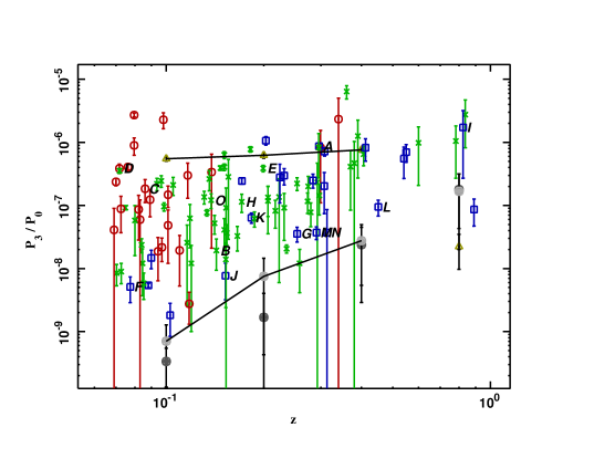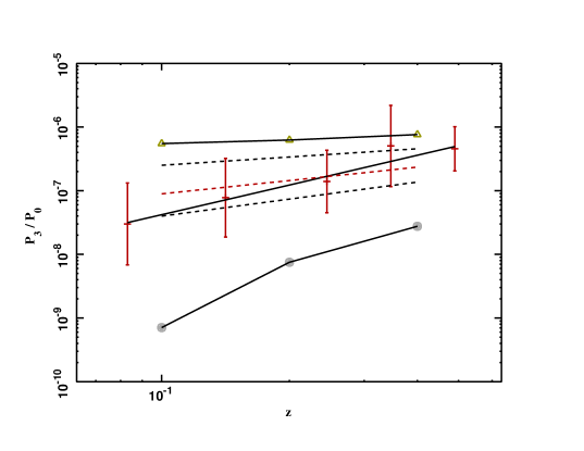
The simulated cool core clusters represent the minimum amount of substructure that can be measured as they are simulated with perfect circular symmetry. This is true for clusters of similar luminosity and exposure. However, the $P_{3}/P_{0}$ values in Table 6 are higher than those of the simulated cool core clusters and above $z=0.3$ most clusters have $P_{3}/P_{0}$ values similar to those of the simulated three-component clusters. This is most clearly seen around $z=0.4$ where the the datapoints cluster around the value of the three-component simulation. Towards $z=0.8$ the simulated irregular cluster shows a decreasing value with redshift due to the smoothing effect introduced by PSF blurring and lack of photons. The datapoints around $z=0.6$ and $z=0.8$ show large $P_{3}/P_{0}$ values around $10^{-6}$, larger than for the simulated clusters.

To investigate further the proposed evolution of $P_{3}/P_{0}$ we restrict the analysis to clusters below $z=0.6$ due to the apparent breakdown in the analysis as seen in the simulated clusters at $z=0.8$. We also exclude the low-luminosity clusters ($L_{bol}<4~{}10^{44}~{}$erg s^-1) from the sample since these are not present at all $z$. We bin the $P_{3}/P_{0}$ values for the remaining clusters in 5 bins of redshift ($z=0$,$0.1$,$0.2$,$0.3$,$0.4$,$0.6$) and fit these datapoints to a straight line in $\log{z}$-$\log{P_{3}/P_{0}}$ space. The binned data is shown along with the best fit line in Figure 11. In order to distinguish between real and apparent evolution we interpolate the slope linearly for values of $\log{P_{3}/P_{0}}$ from the simulated cool core clusters (gray circles) to the simulated clusters with irregular morphology (yellow stars). These interpolated lines are shown as dashed lines in Figure 11 where the red dashed line has the lowest $\chi^{2}$ when compared to the data. Compared to the best line-fit (solid line) the dashed line models have $\Delta\chi^{2}=2.6,1.1$ and $3.3$ respectively (from bottom to top). We conclude that the evolution in $P_{3}/P_{0}$ in addition to the redshift-dependent bias is only slightly more than $1$-$\sigma$ significant.

Table 6Power ratio results

Sample	N.o. objects	$P_{2}/P_{0}(\times 10^{-7})$	$P_{3}/P_{0}(\times 10^{-7})$
$0.069\leq z<0.1$	28	$71\pm 3$	$1.7\pm 0.3$
$0.1\leq z<0.3$	55	$89\pm 5$	$2.2\pm 0.5$
$z\geq 0.3$	18	$65\pm 7$	$7.0\pm 2.8$
cooling clusters	31	$39\pm 2$	$0.29\pm 0.07$

Note. — Average values of the Power Ratios derived in different redshift bins.

Figure 11.— $P_{3}/P_{0}$ values for $L_{bol}\geq 4~{}10^{44}~{}$erg s^-1 clusters up to $z=0.6$ averaged in 5 redshift bins. Best fit line (solid line) is shown along with interpolated trends from the simulated clusters (dashed lines, red dashed line has lowest $\chi^{2}$). Simulated cool core clusters are shown as filled gray circles and simulated irregular (3-core) clusters are shown as yellow stars.

To compare our results with previous work we list our results for the clusters also found in Jeltema et al. (2005) along with their results in Table 7. These values were derived using Chandra data only. We find our values to be consistently about a factor 2 higher with a few exceptions but that they follow the same trend of low to high. This discrepancy could be related to the limited number of photons in the Chandra data causing structures to appear smoother but could also be due to artifacts in our modeling described further in following sections.

Table 7Power ratio comparison

Name	$P_{2}/P_{0}(\times 10^{-7})$	$P_{2}/P_{0}(\times 10^{-7})$	$P_{3}/P_{0}(\times 10^{-7})$	$P_{3}/P_{0}(\times 10^{-7})$
A1413	$58.0$	$192\pm 3$	$0.0525$	$0.19\pm 0.1$
A2034	$14.1$	$84.5\pm 8.4$	$0.476$	$0.41\pm 0.21$
A2218	$27.4$	$72.8\pm 5.6$	$0.233$	$1.14\pm 0.36$
A1914	$15.7$	$32.4\pm 1.0$	$0.709$	$2.45\pm 0.26$
A665	$19.4$	$44.8\pm 3.5$	$2.43$	$7.75\pm 0.77$
A520	$40.7$	$65.3\pm 11.2$	$2.43$	$3.87\pm 0.46$
A963	$5.03$	$8.14\pm 1.32$	$0.342$	$1.34\pm 0.67$
A773	$46.9$	$83.2\pm 11.2$	$-0.125$	$0.82\pm 0.39$
A2261	$4.57$	$12.9\pm 11.4$	$0.201$	$2.79\pm 1.7$
A2390	$58.0$	$149\pm 7$	$0.291$	$2.97\pm 0.86$
A267	$61.4$	$95.8\pm 9.2$	$-0.306$	$0.92\pm 0.64$
RXJ2129.6+0005	$17.6$	$66.1\pm 1.4$	$-0.0814$	$0.21\pm 0.03$
A1758	$188.0$	$502\pm 13$	$1.06$	$0.78\pm 0.32$
ZW3146	$4.42$	$11.6\pm 1.3$	$0.078$	$0.37\pm 0.08$
MS2137-23	$1.81$	$1.47\pm 0.96$	$0.00772$	$0.37\pm 0.49$
CL0016+16	$46.4$	$114\pm 17$	$0.316$	$5.54\pm 2.87$
MS0451.6-0305	$66.1$	$82.3\pm 5.1$	$2.19$	$7.01\pm 2.19$
MS1137.5+6625	$5.24$	$11.5\pm 11.9$	$0.115$	$10.5\pm 7.8$
MS1054.4-0321	$150.0$	$220\pm 73$	$10.3$	$17.3\pm 14.6$
WARPJ0152.7-1357	$264.0$	$2880\pm 260$	$12.4$	$27.6\pm 19.4$
CLJ1226.9+3332	$-0.821$	$11.1\pm 3.2$	$0.77$	$0.87\pm 0.4$

Note. — Comparison of the Power Ratios in our analysis to the results using Chandra data by Jeltema et al. (2005)

5.3. Luminosity-Temperature relation

Using our definition of a cooling cluster, we treat these clusters separately in the subsequent analysis. The remaining clusters are divided into 2 redshift bins; $0.069\leq z<0.2$ and $z\geq 0.2$. This results in 38 low redshift clusters with $\bar{z}=0.11$ and 32 high redshift clusters with $\bar{z}=0.39$.

The X-ray luminosity-temperature relations for these 3 samples are shown in Figure 12. We have used the bolometric luminosity as calculated within a 1 Mpc radius along with the temperatures given in Table 1. The low redshift sample (red circles), the high redshift sample (green stars) and the cooling cluster sample (blue squares) are shown along with their best fit $L_{X}-T$ relations (solid lines). The best fit relations from the non-cooling and cooling samples of Allen & Fabian (1998), at $z=0$, are shown as dashed lines for comparison.

Figure 12.— Luminosity temperature relation for low redshift clusters ($z<0.2$, red circles), high redshift clusters ($z\geq 0.2$, green stars) and cooling core clusters (blue squares). Best fit $L_{X}$-$T$ relations are shown as solid lines and the non-cooling and cooling samples at $z=0$ of Allen & Fabian (1998) are shown as dashed lines.

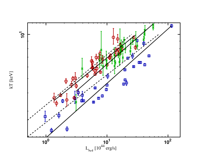Our best fit values of $L_{6}$ and $\alpha_{LT}$ are shown in Table 8, where the bolometric X-ray luminosity is $L_{X}=L_{6}(kT/6~{}$keV$)^{\alpha_{LT}}$. We have added a systematic scatter in $\mathrm{log}(T)$ in order to achieve $\chi^{2}/dof.=1$.

Table 8Luminosity-temperature relation

Sample	$L_{6}$	$\alpha_{LT}$	$\sigma_{syst}(\log(T))$
$0.069\leq z<0.2$	$6.5\pm 0.4$	$2.98\pm 0.19$	0.046
$z\geq 0.2$	$8.9\pm 0.7$	$2.62\pm 0.21$	0.050
cooling clusters	$20.3\pm 2.0$	$2.69\pm 0.18$	0.075

Note. — Best fit parameters for the $L_{X}$-$T$ relation. In addition to the measurement errors, a systematic scatter in $\log(T)$ has been added in order to achieve $\chi^{2}/dof.=1$. The scatter in temperature in the non-cooling sample corresponds to $\sim 0.7~{}$ keV at 6 keV.

It is obvious in this plot that it is of great importance to exclude cooling core clusters since these clusters have much higher $L_{X}$ for a given $T$ compared to non-cooling clusters. It is of particular importance to select these clusters using a method unbiased in redshift. A selection bias at high redshift leading to the failure to identify cooling clusters properly could easily be interpreted as evolution. We have based our selection of cooling clusters on simulated identical clusters at various redshifts, propagating their photons through our detector model to best account for any distance dependent systematic effect.

Fitting the data to a generalized $L_{X}$-$T$ relation with a $z$ dependence;

$$L_{X}=L_{6}~{}\left(\frac{T}{6~{}\mathrm{keV}}\right)^{\alpha_{LT}}~{}(1+z)^{\beta_{LT}},$$ (10)

weak evolution is found with the best fit values for the non-cooling clusters shown in Table 9 along with fits for high luminosity ($L_{bol}\geq 10^{45}$erg s^-1) non-cooling clusters, high $P_{3}/P_{0}$ clusters ($P_{3}/P_{0}\geq 10^{-7}$) and for the cooling clusters separately.

The results for the non-cooling clusters show weak evolution whereas the cooling cluster sample is consistent with no evolution. There is however large intrinsic scatter within the cooling sample. Interestingly, the sample containing the clusters with the highest luminosity substructure (high $P_{3}/P_{0}$, see Section 5.2.1) shows significant evolution with $z$. Slightly higher than that of the non-cooling sample.

It is possible that this has to do with the incompleteness of the sample. A cut on $P_{3}/P_{0}$ selects a larger fraction of high-$z$ clusters, since $P_{3}/P_{0}$ has a weak positive trend with $z$. High redshift clusters tend to be more luminous by selection and this could cause a small bias in the observed evolution. We find that our results for the clusters without cool cores are in good agreement with theoretical models of cluster evolution that are based on balancing gas cooling with feedback at the entropy set by the cooling threshold (Voit et al., 2002; Voit, 2005). This threshold $K_{c}(T,t)$ is the entropy at which constant- entropy gas at temperature $T$ radiates an energy equivalent to its thermal energy in time $t$. These models are also successful in explaining the observed $L_{X}\propto T^{3}$ behavior for clusters, contrary to early assumptions of pure gravitational self-similar collapse, where $L_{X}\propto T^{2}$ was originally expected.

Table 9Redshift dependent luminosity-temperature relation

Sample	$L_{6}$	$\alpha_{LT}$	$\beta_{LT}$	$\sigma_{syst}(\log(T))$
non-cooling	$6.8\pm 0.5$	$2.87\pm 0.14$	$0.50\pm 0.34$	0.037
cooling clusters	$18.8\pm 5.9$	$2.79\pm 0.26$	$0.62\pm 1.47$	0.067
high $L_{bol}$ NC	$7.6\pm 0.7$	$2.81\pm 0.26$	$0.48\pm 0.32$	0.029
high $P_{3}/P_{0}$ NC	$6.4\pm 0.6$	$3.02\pm 0.18$	$0.82\pm 0.42$	0.035

Note. — Best fit parameters for the $L_{X}$-$T$ relation in Eq. 10. In addition to the measurement errors, a systematic scatter in $\log(T)$ has been added in order to achieve $\chi^{2}/dof.=1$. The scatter in temperature in the non-cooling sample corresponds to $\sim 0.5~{}$ keV at 6 keV.

5.3.1 Temperature correlation

Since the temperature two-point correlation function is new, we illustrate its power for four representative clusters that clearly show specific characteristics. $A(r_{k})$ is calculated for all spatial points, with 10 kpc resolution, within radius of 500 kpc of the cluster centroid.

First, we consider a well-known cooling core cluster, Abell 1835 (see Fig. 13, first panel). Here, $A(r_{k})$ is shown as a function of distance scale, $r$. As expected, there is considerable power at small spatial scales, implying a compact structure with temperature clearly different from the rest of the cluster. There is a sharp drop after 500 kpc where the core is no longer visible. Another extreme example is MS1054.4-0321 (Fig. 13, second panel), a highly substructured cluster consisting of multiple components. Here, the amplitude is high, distributed more uniformly over a large range of spatial scales, suggesting multiple high-luminosity components with different temperatures. As a third example, we also show the correlation function for a nearly isothermal cluster, A1689 (Fig. 13, third panel), where small temperature fluctuations lead to lower values across the range of spatial scales. Finally we show the correlation function for A2142 (Fig. 13, fourth panel), where an offset of the cluster core causes the sharp drop seen in A1835 to be absent. The drop is gradual, implying an overall asymmetry in the temperature structure of the cluster.

Figure 13.— The temperature correlation function, $A(r_{k})$ plotted for clusters A1835 (top left), MS1054.4-0321 (top right), A1689 (bottom left) and A2142 (bottom right).

The temperature correlation function $A(r_{k})$ is integrated over $250$-$500~{}$kpc ($A_{1}$) and over $750$-$1000~{}$kpc ($A_{2}$) and this is displayed in Figure 14, plotted against redshift. This shows the magnitude of temperature gradients over small and large scales respectively. These distance ranges are chosen since for the small scales, $250$-$500~{}$kpc, the cooling cores dominate the statistic. To distinguish these fluctuations from larger scale, merger related disturbances we compare it to the $750$-$1000~{}$kpc range where the core cannot be included (since we use a 500 kpc aperture).

Strong cooling clusters such as A1835 and A2204 show large values of $A_{1}$ since the cool cores dominate the small scales. The same objects show low values of $A_{2}$ since these clusters are largely isothermal when the core is excluded. The same is true for our simulated cool core clusters, while the small scales cannot quite be resolved at high $z$. In contrast, disturbed clusters such as RXJ0658-55 or MS1054.4-0321 show generally lower values of $A_{1}$ and larger values of $A_{2}$ whereas nearly isothermal clusters such as A1689 or A1413 show low values for both. With the exception of a few low luminosity clusters at low redshift, large scale temperature structure ($A_{2}$) can be seen to increase slightly with redshift above $z=0.2$ when compared to the simulated clusters. There is also an apparent drop in the temperature structure for smaller scales ($A_{1}$).

We note that the decrease in $A_{1}$ with redshift can be partly due to smoothing of the core caused by the PSF and loss of photons as seen in the evolution in the simulated clusters in Figure 14. However, it is unlikely that this effect is the cause of the increase in $A_{2}$ since temperature features are likely to be washed out by this effect. This is seen in the trend of $A_{2}$ for the simulated clusters.

Figure 14.— Temperature correlations for scales $250-500~{}$kpc ($A_{1}$) vs redshift (left panel) and $750-1000~{}$kpc ($A_{2}$) vs $z$ (right panel). The different symbols represent luminosity (red circles $\geq 10^{43}~{}$erg s^-1, green stars $\geq 4~{}10^{44}~{}$erg s^-1, and blue squares $\geq 2~{}10^{45}~{}$erg s^-1). Simulated cool core clusters are shown as filled gray circles. Letters from A to O denote a few selected clusters (see Figure 7).

Figure 15.— Temperature correlations for scales $750-1000~{}$kpc ($A_{2}$) plotted against $250-500~{}$kpc ($A_{1}$) scales. Here the different symbols represent redshift (red circles $0.069\leq z<0.1$, green stars $0.1\leq z<0.3$, and blue squares $z\geq 0.3$). Simulated cool core clusters are shown as filled gray circles. Letters from A to O denote a few selected clusters (see Figure 7).

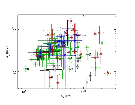In Figure 15 we plot $A_{2}$ against $A_{1}$ to show the separation of “relaxed” cool core clusters (lower right) from disturbed clusters (upper left).

5.4. Notes on individual clusters

In this section we describe breifly a few selected clusters in our sample, comparing our findings with previous results. The luminosity and temperature maps of these clusters are presented in Figures 16 to 32.

5.4.1 Abell 1068

A high resolution temperature map of Abell 1068, using Chandra data, was previously presented in Wise et al. (2004) who find an large degree of substructuring within the central $80~{}\arcsec\times 80~{}\arcsec$ with temperatures varying between 2.5 and 6 keV. We find that this agrees well with our map in Figure 16, although the spatial resolution is not as high as in the Chandra map. The size of the $80~{}\arcsec\times 80~{}\arcsec$ region can be estimated using 4 times the PSF width in Figure 16. In a radial temperature profile derived from the XMM-Newton data, Snowden et al. (2008) find a central temperature of $3.1~{}$keV increasing to $5.3~{}$keV around $0.4~{}r_{500}$ and dropping to $2.2~{}$keV around $0.8~{}r_{500}$ ($\sim 800~{}$kpc). In our map we find no indication of such a drop in $T$. We note, however, that due to the low cluster flux at these radii, the error on the temperature in the map is large ($\sim 3~{}$keV). There may also be some associated systematic effects (see Section 6). The average temperature of the cluster that we find from a simple spectral analysis is $3.81^{+0.08}_{-0.07}~{}$keV.

5.4.2 Abell 1413

Early studies of the temperature profile of Abell 1413 using XMM-Newton data find a central temperature of approximately $7~{}$keV declining to $6~{}$keV out to 1 Mpc radius (Pratt & Arnaud, 2002). Snowden et al. (2008) find a similar trend with a central temperature of $7.7~{}$keV declining to $5.7~{}$keV out to $\sim 1~{}$Mpc. Our temperature map (Figure 17) exhibits a large degree of small scale substructure in this otherwise smooth surface brightness distribution with temperatures varying between $7$ and $9~{}$keV. We do not see a clear temperature drop with increasing radius but rather a large degree of asymmetry. We find an average spectral temperature of $7.30^{+0.19}_{-0.19}~{}$keV.

5.4.3 Abell 1689

The temperature map of Abell 1689 (Figure 18) is in good agreement with our earlier analysis of the XMM-Newton data (Andersson & Madejski, 2004; Andersson et al., 2007). Snowden et al. (2008) find a slightly higher temperature of 11.6 keV around $0.1~{}r_{500}$ ($\sim 200~{}$kpc) whereas at other radii the results are consistent with ours with fluctuations from $8$ to $10~{}$keV. The average spectral temperature is $9.07^{+0.17}_{-0.12}~{}$keV.

5.4.4 Abell 1750

The XMM-Newton data for Abell 1750, consisting of two subclusters, was analyzed by Belsole et al. (2004) who find temperatures varying between $3$ and $6~{}$keV within the double-cluster. The temperature structure overall is in good agreement with our temperature map while we find temperatures varying from $4.5$ to $8.5~{}$keV. This is likely related to the bias described in Section 6.4. We find that the larger subcluster (pictured center in Fig. 19) is slightly hotter ($5.5~{}$keV) compared to the northern subcluster ($4.5~{}$keV) with the gas in between having a temperature of $8~{}$keV. Belsole et al. (2004) find these temperatures to be $2.8$, $3.9$ and $5.1~{}$ keV respectively. In a simple spectral fit we find the average temperature of A1750 to be $4.45^{+0.13}_{-0.13}~{}$keV.

5.4.5 Abell 1758

Abell 1758 is a complicated system consisting of a northern and a southern component, separated by 2 Mpc in the plane of the sky, each of which, in turn, consists of two separate subclusters. We have limited our analysis to the northern component A1758N (See Fig. 20). The Chandra and XMM-Newton data of A1758 have been analyzed earlier by David & Kempner (2004) who conclude that A1758N is in the late stages of a large impact parameter merger of two 7 keV clusters. The hardness ratio map presented in David & Kempner (2004) is qualitatively in good agreement with our temperature map. For their spectral fits in four separate regions they find temperatures of $7.2$, $6.6$, $7.2$ and $9.8~{}$ keV for the “northwest wake”, “southeast wake”, “core” and “halo” using the XMM-Newton data. The values for the same regions in our temperature map are systematically approximately 1 keV higher. In our overall spectral fit we find a temperature of $9.16^{+0.39}_{-0.43}~{}$keV.

5.4.6 Abell 1775

Abell 1775 is a nearby ($z=0.072$), low mass cluster with high velocity dispersion, containing a pair of massive galaxies at the center (Figure 21). Studying the velocity distribution of the galaxies in this cluster, Oegerle et al. (1995) conclude that it, in fact, consists of two smaller subclusters that are in the process of merging. In our temperature map, we can see an arc of the coldest gas extending to the east of the cluster center, possibly a remnant of a subcluster core. In this low mass cluster, the surface brightness becomes low outside 500 kpc and the temperature map outside of this radius is not reliable. Within 500 kpc we find the gas temperature varying in the 4 to 7 keV range, biased upward by effects described in Section 6.4. Adapting the prior range of the temperature distribution in this case to better accommodate for low temperature gas would give a more accurate result. Snowden et al. (2008) find a central temperature of $4.3~{}$keV decreasing to $3.5~{}$keV around $0.4~{}r_{500}$ ($\sim 600~{}$kpc). In our overall spectral fit we find a temperature of $3.70^{+0.10}_{-0.06}~{}$keV.

5.4.7 Abell 1835

Abell 1835 is a massive cluster with a pronounced cool core and a relaxed morphology. Majerowicz et al. (2002) find a central temperature of $4.1~{}$keV increasing to $8.5~{}$keV near 1 Mpc using XMM-Newton data. Snowden et al. (2008) find a central temperature of $6.1~{}$keV, increasing to $10.5~{}$keV just outside the cluster core and decreasing to $7.7~{}$keV out to 1 Mpc using the same data. This is in good agreement with our temperature map shown in Figure 22. In a simple spectral fit we find the average temperature of A1835 to be $7.14^{+0.10}_{-0.11}~{}$keV.

5.4.8 Abell 2029

Using an early Chandra observation of A2029, Lewis et al. (2002) find a central temperature as low as $4~{}$keV within 10 kpc increasing to approximately 9 keV out to 300 kpc. Using the same data, Clarke et al. (2004) find a disturbed core within a 20 kpc radius with some spatial correlation to the central radio emission. In our temperature map in Figure 23 we find no significant central substructuring on the scales we are probing with the XMM-Newton data. Bourdin & Mazzotta (2008) find a central temperature of $5.7~{}$keV and a large degree of temperature substructure with fluctuations between $7$ and $9.5~{}$keV in their temperature map out to $600~{}$ kpc, generated using the XMM-Newton data. While in good quantitative agreement with the radial trend in our temperature map, we find no sign of the hot or cold substructures in our map. In our overall spectral fit we find a temperature of $6.88^{+0.11}_{-0.08}~{}$keV.

5.4.9 Abell 2142

Markevitch et al. (2000) first argued that A2142 contains a “cold front”, a steep nonaxisymmetric X-ray flux gradient and a steep temperature gradient originally believed to be due to a low-entropy remnant of a recently merged subcluster. Tittley & Henriksen (2005) argue that this “cold front” is due to oscillatory motions of the core after a merger event. Our temperature map (Figure 24) shows a central temperature around $7.5~{}$keV with a plume-like structure of $8.5~{}$keV gas extending north and a steep temperature gradient, aligned with the sharp trend in surface brightness to the north-west, increasing to $11.5~{}$keV. This agree well with the results of Markevitch et al. (2000), with the exception of the central $5~{}$keV gas which we do not detect. We find an overall spectral temperature of A2142 to be $8.15^{+0.24}_{-0.28}~{}$keV.

5.4.10 Abell 2204

Abell 2204 is a massive cool core cluster with a regular morphology. Sanders et al. (2005) find the temperature of the core region to be $3.26\pm 0.20~{}$keV. The temperature map of Sanders et al. (2005) shows a gradually increasing temperature to $\sim 10~{}$keV at 100 kpc, continuing up to $16~{}$keV around 400 kpc after which it drops again to around 7 keV. The trend is continuous, with the exception of an arc-shaped region of hot gas extending around the northern part of the cluster at 50 kpc where the temperature suddenly jumps to 14 keV. Our map in Figure 25 shows a similar trend with a central temperature of $4.5~{}$keV gradually increasing to $10~{}$keV around 300 kpc where after it drops again to $7~{}$keV at 1 Mpc. We find no signs of the hotter gas around 50 kpc. Reiprich et al. (2008) also find a similar radial profile using data from Chandra, XMM-Newton and Suzaku telescopes with a sharp increase in temperature outside of the core and a gradual decline out to the virial radius where a temperature of 4 keV is measured. In our overall spectral fit we find a temperature of $6.44^{+0.08}_{-0.09}~{}$keV, dominated by the emission from the core.

5.4.11 Abell 520

A detailed temperature map of A520, using a short Chandra observation, was first presented in Markevitch et al. (2003). The map shows the southwestern cluster core having a temperature of approximately $5~{}$keV while the main body of the cluster exhibits an irregular morphology with temperatures varying from 6 to 14 keV. Using a longer observation, Markevitch et al. (2005) detect a temperature drop in the southwest quadrant, from $11.5^{+6.7}_{-3.1}~{}$keV at $400-600~{}$kpc distance from the center to $4.8^{+1.2}_{-0.8}~{}$keV at $600-1000~{}$kpc. We do not find any evidence for such a temperature drop. This is most likely due to the fact that the surface brightness is low in this quadrant at this large radius. Directly south of the main cluster, we see a region of possibly shocked gas at $11~{}$keV and this appears to be the source of the hottest emission in this cluster (see Figure 26). In the overall spectral fit we find this cluster has an average temperature of $8.45^{+0.33}_{-0.26}~{}$keV.

5.4.12 MS0451.6-0305

The temperature map in Figure 27 reveals a low-temperature (7 keV) structure east of the main cluster (10 keV). It is possible that this component represents a subcluster in the process of merging with the main cluster, or perhaps a less massive cluster in projection. This feature can be seen in the maps of surface brightness presented in Donahue et al. (2003), where the soft-band image is seen to extend further east than the hard-band map. Donahue et al. (2003) further find a central temperature ($r<31\arcsec$) of $10.3^{+2.2}_{-1.5}~{}$keV and an outer temperature ($31\arcsec<r<85\arcsec$) of $9.8^{+2.5}_{-1.7}~{}$keV. In our overall spectral fit we find a temperature of $10.02^{+0.80}_{-0.60}~{}$keV in good agreement with their results.

5.4.13 MS1054.4-0321

MS1054.4-0321 has been studied previously with Chandra and XMM-Newton. Gioia et al. (2004) find an overall temperature of $7.2^{+0.6}_{-0.7}~{}$keV using the XMM data while Jee et al. (2005) find an overall temperature of $8.9^{+1.0}_{-0.8}~{}$keV using the Chandra data. Jee et al. (2005) also find the temperature of the western peak to be $7.5^{+1.4}_{-1.2}~{}$keV, the central peak to be $10.7^{+2.1}_{-1.7}~{}$keV and an overall positive gradient in their temperature map from west to east. We confirm the presence of a temperature gradient, seen rising from 9 to 11 keV in Figure 28. In our overall spectral fit we find a temperature of $9.20^{+1.26}_{-1.03}~{}$keV in good agreement with the Chandra results.

5.4.14 MS2137-23

MS2137-23 is a strong gravitational lensing cluster with a well defined central cool core. In the temperature map in Figure 29 we see the temperature increase from 5 to 8 keV within 500 kpc radius. The map exhibits a low degree of asymmetry which appears to increase with radius. In a deprojected temperature profile using a Chandra observation, Arabadjis et al. (2004) find a central ($\sim<50~{}$kpc) temperature of 4 keV rising to around 7 keV at 150 kpc radius and decreasing again at larger radii. An offset datapoint at 250 kpc radius shows a temperature of $12.5\pm 4.5~{}$keV. Our overall spectral fit shows a temperature of $4.67^{+0.17}_{-0.19}~{}$keV, clearly showing the dominance of the cool core emission.

5.4.15 RXJ0658-55

For a detailed discussion on the temperature structure of RXJ0658-55, see Andersson et al. (2007). Our maps of luminosity and temperature are shown in Figure 30.

5.4.16 RXJ1347-1145

The temperature map in Figure 31 shows a central temperature of $9~{}$keV increasing to $11.5~{}$keV within 500 kpc and decreasing again towards 1000 kpc radius. The temperature map further shows a lack of the hottest emission in the north quadrant of the cluster. We compare our results with the radial temperature profile and map of Gitti & Schindler (2004), derived from the XMM-Newton data. The temperature profile shows an overall good agreement with our results, however, the temperature map of Gitti & Schindler (2004) identifies a region of hot ($\sim 17~{}$keV) emission approximately 150 kpc south-east if the core. This region appears in our map as a region of $11.5~{}$keV emission aligned with the elongation of the surface brightness to the SE. Our map also shows less substructure overall. We find this massive cluster has an overall spectral temperature of $11.44^{+0.26}_{-0.29}~{}$keV.

5.4.17 ZW3146

The temperature map of the cool core cluster ZW3146 (Figure 32) reveals a central temperature of $5.5~{}$keV increasing to approximately $9~{}$keV at 500 kpc. At larger radii the temperature appears to increase further, however, here the measurement is uncertain. Using XMM-Newton data, Kausch et al. (2007) find a temperature gradient from 4.7 to 7 keV up to $1~{}$Mpc with most of the colder emission being localized within $100~{}$kpc. Their temperature map shows fluctuations between $4.5$ and $9$ keV in within 200 kpc. We do not see these fluctuations and conclude that the cluster has a relatively relaxed morphology with a smooth temperature gradient. The surface brightness contours have tighter spacing to the south-east which may indicate recent core motion relative to the cluster as a whole. Our overall spectral fit shows a temperature of $6.21^{+0.14}_{-0.10}~{}$keV.

6. Systematic effects

6.1. Selection bias

Since the cluster sample was selected using all the public XMM data available at the time, it does not consist of a representative subset of clusters in general in the universe. However, many studies, and observation proposals, are based on either the most regular known clusters or the most complex. Hence, the sample should contain both these extremes of the cluster population which is what is compared in this work.

6.2. Background modeling

The X-ray background is modeled as opposed to subtracted which is the usual procedure in standard spectral modeling of extended X-ray sources. This introduces an uncertainty different from the unsubtracted background flux which is common when dealing with combinations of several sources of background with different spatial and spectral distributions. Here, the distortions of different backgrounds are modeled correctly, but instead, there is the possibility of cluster particles mimicking the background flux. This effect is small since the backgrounds are present across the entire field which is not the case for the majority of the cluster emission since all clusters are modeled out to at least 1 Mpc where the cluster emission tends to be faint. The low cluster flux at this radius does, however, impact on the precision of the temperature measurements at large radii. The nature of this uncertainty is seen in some temperature maps of median temperature as it reverts to the mean of the prior, which in this case is 7.75 keV.

The spectral shape of the instrumental background also means that it is not easily modeled by cluster particles. The particle background has a nearly flat spectral shape across the entire energy range whereas the X-ray photons are modulated by the energy dependent effective area of the X-ray mirrors. This makes it statistically favorable to model these events using the background model which is not affected by mirrors as opposed to using the SPI particles.

In order to estimate the effect of the background modeling on the temperature at large radii we compare the temperature correlation results, $A_{1}$ and $A_{2}$, for the simulated regular clusters with and without background. These are shown as filled circles in dark and light gray respectively in Figures 14 and 15. The inclusion of background leads to an overestimation of approximately 25% in $A_{1}$ and 35% in $A_{2}$. This is comparable to the 1-$\sigma$ statistical errors and since the effect appears to be relatively independent of redshift we conclude that it does not affect the evolution of the temperature correlation.

6.3. Point-sources

Point sources can significantly alter maps of cluster luminosity and temperature. In the cases where we can identify the point sources from the original event file we remove the flux from these sources using the technique described above (Section 4.1, Figure 5). When a point source cannot be resolved it can have a large impact on the temperature maps even if the effect on the luminosity map is not visible. Ideally, Chandra data of the same cluster should be used in combination to identify the positions of point sources and to verify the accuracy of temperature features. Chandra data is however not available for all clusters in the sample and this type of analysis is beyond the scope of this work.

6.4. Temperature bias

As mentioned earlier, the average temperature from the SPI modeling becomes slightly higher than when standard analysis routines are applied. This effect stems from the fact that we are using multiple particles in our modeling. Since the particles are extended and hundreds of particles are required to model a single cluster there will be multiple overlapping cluster particles at any given position. Each particle has a separate temperature and set of elemental abundances and this means that the model is inherently multi-phase. There are many combinations of thermal spectra that can be constructed to agree with the observed data and the final model consists of a wide range of phases at each spatial position. This range is very much dependent on the prior range for the parameter in question. Here, these ranges are visualized by making use of the median of the range at each spatial coordinate and this value again depends on the prior range. Since the measured differences of thermal spectra in XMM become smaller with increasing temperature the median is naturally biased towards the higher part of the prior. This may lead to a potential luminosity bias in the bolometric correction since the luminosities are calculated separately for each smoothed particle which will cause a higher luminosity if the temperature is higher. We estimate this offset to be less than $\sim 20$ % based on a comparison when using the temperature from the “standard” analysis in the bolometric correction.

6.5. Modeling artifacts

Since the modeling itself is based on particles, even if between 100 and 1000 particles are required, there is a possibility for particle artifacts appearing in the luminosity and temperature maps. The cluster particles are constantly moving within the parameter space and interchanging positions with each other, and averaging over many Markov chain samples reduces this effect. However, since we are limited by CPU resources (see also Section 4.2) and only 250 samples are used in the error calculation these artifacts may still show up in the maps as lumpy structures and this may have a small effect increasing the power ratios. In comparing power ratios calculated from maps using 1500 samples with ones generated using 250 samples we establish that this effect corresponds to about a 20 % increase for ratios ($P_{2}/P_{0}$ or $P_{3}/P_{0}$) between $10^{-8}$ and $10^{-7}$ and less for larger values. However, this is not sufficient to explain the discrepancy in the comparison with the values from Jeltema et al. (2005).

6.6. Trends of the simulated clusters

In many of the plots, the trends in the relevant parameters with $z$ for the simulated cool core clusters appear similar to the evolution for the sample as a whole. In most cases, the trend for the simulations only represents the minimum disturbance that can be measured and the similarity does not necessarily mean that the evolution is not real. In fact, we see from our simulations of irregular clusters that the trend for a cluster with high $P_{2}/P_{0}$ or $P_{3}/P_{0}$ is much more stable than that of the circularly symmetric clusters. Ideally, to make a more rigorous claim of evolution, clusters of many different morphologies should be simulated and the apparent evolution analyzed separately. This will be the subject of future work and we are limited here, again, by CPU constraints. Markov chains should also be run for several more iterations to limit model noise.

7. Discussion and conclusions

We have applied a novel technique for X-ray galaxy cluster modeling to a large sample of XMM observed galaxy clusters in order to identify clusters with cooling cores and to study the redshift dependence of cluster substructure and the luminosity-temperature relation. We also developed a new statistic to quantify thermal substructure and to identify and distinguish cooling core clusters from isothermal and thermally disturbed clusters. We note here that while this technique is important in identifying clusters for which mass measurement can be used for cosmological applications, in its present form it is not capable of estimating cluster masses. However, a straightforward extension of it, with additional assumptions, should allow the determination of three-dimensional density and temperature of the cluster, and thus the mass of both gas and dark matter content.

The number of cooling core clusters appears to be lower at high $z$ with 32 % identified as cooling clusters at $z<0.1$, 36 % at $0.1\leq z<0.3$ and 11 % at $z\geq 0.3$. This suggests that the formation of cooling cores in clusters is a recent phenomenon. However, due to the low number of clusters and various selection effects these percentages are uncertain.

7.1. L-T relation

The derived luminosity-temperature relation for clusters clearly shows a large offset for cooling core clusters, as expected. This highlights the importance of applying a redshift dependent criterion when excluding these sources. In contrast to previous work we do not attempt to correct for cooling cores by applying some standardized central profile. Instead we fit the relation for cooling clusters separately (cf. Allen & Fabian, 1998) and find a similar slope of $\sim 3$ but with a normalization $\sim 3$ times higher than for the non-cooling sample. The normalization of our $L_{X}$-$T$ relation for cool core clusters is $\sim 50\%$ higher for our sample compared to the findings of Allen & Fabian (1998). This is likely due to the use of ROSAT and Asca data to determine temperatures and luminosities, where cool core clusters would hard to model with the low spatial resolution and the limited energy band.

We also note that the scatter in the $L_{X}$-$T$ relation is greater for cooling core clusters. We detect weak evolution in the non-cooling $L_{X}-T$ relation $\propto(1+z)^{0.50\pm 0.34}$ in good agreement with self similar predictions and with an average slope of $\alpha_{LT}=2.87\pm 0.14$. This is in contrast to the findings of Vikhlinin et al. (2002) who detect strong evolution $\propto(1+z)^{1.5\pm 0.3}$. Due to the limited observable volume available at low $z$, high luminosity clusters are observed at mostly high redshifts. This could create a $\alpha_{LT}$-$\beta_{LT}$ bias. We note also that when studying $\beta_{LT}$ for the cluster sample with $P_{3}/P_{0}>10^{-7}$, the sample shows significant evolution. This may be an important effect to account for in large surveys relying on the $L_{X}$-$T$ relation to measure the mass function of clusters over a range in $z$. Clearly, the $L_{X}$-$T$ relation has to be measured in greater detail with larger samples of well exposed clusters in order to reach a consensus of its evolution. To measure the mass function of clusters to constrain cosmological parameters the knowledge of this evolution is crucial.

7.2. Structure quantification

The power ratio analysis was applied uniformly for the 101 clusters within a 500 kpc radius. We find no significant increase in $P_{2}/P_{0}$ with $z$ but detect an increase in $P_{3}/P_{0}$ implying a higher level of substructure at high redshift. Our sample of cooling core clusters shows significantly lower values of $P_{2}/P_{0}$ and $P_{3}/P_{0}$ than the non-cooling sample, which is not surprising since cooling clusters generally are the most dynamically relaxed clusters.

Comparing this quantification of cluster structure with simulations of spherical clusters we show that all clusters in our sample are far from spherical, as determined by the value of $P_{2}/P_{0}$ and should not be modeled as such. This is easily realized when viewing the luminosity maps in Figures 16-32 which exhibit a large degree of ellipticity. The large amount of features visible in the temperature maps confirm that a large number of processes govern the properties of the intra-cluster medium, that cluster merging can give rise to highly complex thermal structure and that temperature seldom is a simple function of radius.

The SPI method inherently lends itself to a study of temperature structure of clusters, and to take advantage of it, we design a statistic, the “temperature two-point correlation”, capable of distinguishing between cooling clusters, isothermal clusters and clusters with significant temperature differences over large distances, such as merging clusters. The analysis using this function hints at an increase in the large scale thermal structure of clusters with redshift, indicating more frequent merging in a denser universe. This indication could be confirmed using a joint approach utilizing both XMM-Newton and Chandra datasets.

8. Acknowledgments

K.A. acknowledges financial support from the Göran Gustavsson Foundation for Research in Natural Sciences and Medicine. This research was supported by NASA XMM-Newton observing grants NNX06AE39G and NNX07AE93G, and by the Department of Energy contract to SLAC no. DE-AC3-76SF00515.

Figure 16.— $2\times 2$ Mpc images of the bolometric luminosity, in units of $10^{44}~{}$erg s^-1 $(\arcsec)^{-2}$ (left panel), and temperature, in keV (right panel), for Abell 1068. The size of the 500 kpc region used for power ratio analysis and two-point temperature correlation analysis is shown along with the size of the PSF (10$\arcsec$ radius) .

Figure 17.— $2$ Mpc $\times 2$ Mpc field showing luminosity (left) and temperature (right) maps of Abell 1413.

Figure 18.— $2$ Mpc $\times 2$ Mpc field showing luminosity (left) and temperature (right) maps of Abell 1689.

Figure 19.— $2$ Mpc $\times 2$ Mpc field showing luminosity (left) and temperature (right) maps of Abell 1750.

Figure 20.— $2$ Mpc $\times 2$ Mpc field showing luminosity (left) and temperature (right) maps of Abell 1758.

Figure 21.— $2$ Mpc $\times 2$ Mpc field showing luminosity (left) and temperature (right) maps of Abell 1775.

Figure 22.— $2$ Mpc $\times 2$ Mpc field showing luminosity (left) and temperature (right) maps of Abell 1835.

Figure 23.— $2$ Mpc $\times 2$ Mpc field showing luminosity (left) and temperature (right) maps of Abell 2029.

Figure 24.— $2$ Mpc $\times 2$ Mpc field showing luminosity (left) and temperature (right) maps of Abell 2142.

Figure 25.— $2$ Mpc $\times 2$ Mpc field showing luminosity (left) and temperature (right) maps of Abell 2204.

Figure 26.— $2$ Mpc $\times 2$ Mpc field showing luminosity (left) and temperature (right) maps of Abell 520.

Figure 27.— $2$ Mpc $\times 2$ Mpc field showing luminosity (left) and temperature (right) maps of MS0451.6-0305.

Figure 28.— $2$ Mpc $\times 2$ Mpc field showing luminosity (left) and temperature (right) maps of MS1054.4-0321.

Figure 29.— $2$ Mpc $\times 2$ Mpc field showing luminosity (left) and temperature (right) maps of MS2137-23.

Figure 30.— $2$ Mpc $\times 2$ Mpc field showing luminosity (left) and temperature (right) maps of RXJ0658-55.

Figure 31.— $2$ Mpc $\times 2$ Mpc field showing luminosity (left) and temperature (right) maps of RXJ1347-1145.

Figure 32.— $2$ Mpc $\times 2$ Mpc field showing luminosity (left) and temperature (right) maps of ZW3146.

References

- Allen & Fabian (1998) Allen, S. W., & Fabian, A. C. 1998, MNRAS 297, L57
- Allen et al. (2008) Allen, S. W., Rapetti, D. A., Schmidt, R. W., Ebeling, H., Morris, R. G., & Fabian, A. C. 2008, MNRAS, 383, 879
- Anders & Grevesse (1989) Anders, E., & Grevesse, N. 1989, Geochim. Cosmochim. Acta, 53, 197
- Andersson & Madejski (2004) Andersson, K. & Madejski, G. 2004, ApJ 607, 190.
- Andersson et al. (2007) Andersson, K., Peterson, J. R., & Madejski, G. 2007, ApJ, 670, 1010
- Arabadjis et al. (2004) Arabadjis, J. S., Bautz, M. W., & Arabadjis, G. 2004, ApJ, 617, 303
- Arnaud (1996) Arnaud, K. A. 1996, Astronomical Data Analysis Software and Systems V, 101, 17
- Arnaud & Evrard (1999) Arnaud, M. & Evrard, A. E. 1999, MNRAS, 305, 631
- Arnaud et al. (2005) Arnaud, M., Pointecouteau, E., & Pratt, G. 2005, astro-ph/0502210
- Belsole et al. (2004) Belsole, E., Pratt, G. W., Sauvageot, J.-L., & Bourdin, H. 2004, A&A, 415, 821
- Bourdin & Mazzotta (2008) Bourdin, H., & Mazzotta, P. 2008, A&A, 479, 307
- Buote & Tsai (1995) Buote, D. A., & Tsai, J. C. 1995, ApJ, 452, 522
- Clarke et al. (2004) Clarke, T. E., Blanton, E. L., & Sarazin, C. L. 2004, ApJ, 616, 178
- Chen et al. (2007) Chen, Y., Reiprich, T. H., Böhringer, H., Ikebe, Y., & Zhang, Y.-Y. 2007, A&A, 466, 805
- David & Kempner (2004) David, L. P., & Kempner, J. 2004, ApJ, 613, 831
- Dickey & Lockman (1990) Dickey, J. M., & Lockman, F. J. 1990, ARA&A 28, 215.
- Donahue et al. (2003) Donahue, M., Gaskin, J. A., Patel, S. K., Joy, M., Clowe, D., & Hughes, J. P. 2003, ApJ, 598, 190
- Finoguenov et al. (2005) Finoguenov, A., Böhringer, H., & Zhang, Y.-Y. 2005, A & A, 442, 827
- Gioia et al. (2004) Gioia, I. M., Braito, V., Branchesi, M., Della Ceca, R., Maccacaro, T., & Tran, K.-V. 2004, A&A, 419, 517
- Gitti & Schindler (2004) Gitti, M., & Schindler, S. 2004, A&A, 427, L9
- Jee et al. (2005) Jee, M. J., White, R. L., Ford, H. C., Blakeslee, J. P., Illingworth, G. D., Coe, D. A., & Tran, K.-V. H. 2005, ApJ, 634, 813
- Jeltema et al. (2005) Jeltema, T. E., Canizares, C. R., Bautz, M. W., & Buote, D. A. 2005, ApJ, 624, 606
- Kaastra (1992) Kaastra, J. S. 1992, An X-Ray Spectral Code for Optically Thin Plasmas (Internal SRON-Leiden Report, ver. 2.0)
- Kausch et al. (2007) Kausch, W., Gitti, M., Erben, T., & Schindler, S. 2007, A&A, 471, 31
- Kravtsov et al. (2006) Kravtsov, A. V., Vikhlinin, A., & Nagai, D. 2006, ApJ, 650, 128
- Kuntz & Snowden (2000) Kuntz, K. D., & Snowden, S. L. 2000, ApJ, 543, 195
- Liedahl et al. (1995) Liedahl, D. A., Osterheld, A. L., & Goldstein, W. H. 1995, ApJ, 438, L115
- Lewis et al. (2002) Lewis, A. D., Stocke, J. T., & Buote, D. A. 2002, ApJ, 573, L13
- Majerowicz et al. (2002) Majerowicz, S., Neumann, D. M., & Reiprich, T. H. 2002, A&A, 394, 77
- Markevitch et al. (2000) Markevitch, M., et al. 2000, ApJ, 541, 542
- Markevitch et al. (2003) Markevitch, M., Vikhlinin, A., & Forman, W. R. 2003, Astronomical Society of the Pacific Conference Series, 301, 37
- Markevitch et al. (2005) Markevitch, M., Govoni, F., Brunetti, G., & Jerius, D. 2005, ApJ, 627, 733
- Markevitch & Vikhlinin (2007) Markevitch, M., & Vikhlinin, A. 2007, Phys. Rep., 443, 1
- Maughan et al. (2008) Maughan, B. J., Jones, C., Forman, W., & Van Speybroeck, L. 2008, ApJS, 174, 117
- McNamara et al. (2004) McNamara, B. R., Wise, M. W., & Murray, S. S. 2004, ApJ, 601, 173
- Mewe et al. (1985) Mewe, R., Gronenschild, E. H. B. M., & van den Oord, G. H. J. 1985, A&AS, 62, 197
- Mewe et al. (1986) Mewe, R., Lemen, J. R., & van den Oord, G. H. J. 1986, A&AS, 65, 511
- Morrison & McCammon (1983) Morrison, R. & McCammon, D. 1983, ApJ, 270, 119
- Oegerle et al. (1995) Oegerle, W. R., Hill, J. M., & Fitchett, M. J. 1995, AJ, 110, 32
- Peterson & Fabian (2006) Peterson, J. R., & Fabian, A. C. 2006, Phys. Rep., 427, 1
- Peterson, Marshall, & Andersson (2007) Peterson, J. R., Marshall, P. J., & Andersson, K. E. 2007, ApJ 655, 109.
- Pratt & Arnaud (2002) Pratt, G. W., & Arnaud, M. 2002, A&A, 394, 375
- Reiprich et al. (2008) Reiprich, T. H., et al. 2008, arXiv:0806.2920
- Sanders et al. (2005) Sanders, J. S., Fabian, A. C., & Taylor, G. B. 2005, MNRAS, 356, 1022
- Schuecker et al. (2001) Schuecker, P., Böhringer, H., Reiprich, T., & Feretti, L. 2001, A & A, 378, 408
- Snowden et al. (2008) Snowden, S. L., Mushotzky, R. F., Kuntz, K. D., & Davis, D. S. 2008, A&A, 478, 615
- Tittley & Henriksen (2005) Tittley, E. R., & Henriksen, M. 2005, ApJ, 618, 227
- Vikhlinin et al. (2002) Vikhlinin, A., VanSpeybroeck, L., Markevitch, M., Forman, W. R., &, Grego L. 2002, ApJL, 578, L107
- Vikhlinin et al. (2006a) Vikhlinin, A., Kravtsov, A., & Forman, W. 2006a, ApJ, 640, 691
- Vikhlinin et al. (2006b) Vikhlinin, A., Burenin, R., Forman, W. R., Jones, C., Hornstrup, A., Murray, S. S., & Quintana, H. 2006b, ArXiv Astrophysics e-prints, arXiv:astro-ph/0611438
- Voit et al. (2002) Voit, G. M., Bryan, G. L., Balogh, M. L., & Bower, R. G. 2002, ApJ, 576, 601
- Voit (2005) Voit, G. M. 2005, Reviews of Modern Physics, 77, 207
- Wise et al. (2004) Wise, M. W., McNamara, B. R., & Murray, S. S. 2004, ApJ, 601, 184