Entanglement enhanced bit rate over multiple uses of a lossy bosonic channel with memory

Abstract

We present a study of the achievable rates for classical information transmission via a lossy bosonic channel with memory, using homodyne detection. A comparison with the memoryless case shows that the presence of memory enhances the bit rate if information is encoded in collective states, i.e. states which are entangled over different uses of the channel.

I Introduction

One of the tasks of quantum information theory is to evaluate the capacity of quantum channels for the transmission of classical information. Recently, much attention has been devoted to the study of quantum channels with memory (see e.g. werner and the references therein). There are evidences that memory effects can enhance the classical capacity in both the cases of discrete discr and continuous cont variables. Bosonic Gaussian channels provide a fertile benchmark for the study of quantum channels with continuous alphabet holevo1 ; holevo2 . Here we consider a model of lossy bosonic memory channel introduced in oleg , based on the general scheme proposed in mancini (see also Ruggeri ). In this kind of model, memory effects come from the interaction with a common environment containing correlations. In spite of the fact that each channel belonging to this family is unitary equivalent to a memoryless one, the presence of energy constraints can break the unitary symmetry, leaving the problem of evaluating capacities open (see mancini ). A specific instance of a channel belonging to that family is obtained by specifying the state of the environment. Here we consider a multimode squeezed vacuum with one free parameter expressing the degree of squeezing, this parameter in turn determines the amount of memory contained in the channel.

The aim of this paper is to evaluate the maximum achievable transmission rate using homodyne detection. A similar analysis was already presented in oleg , where the maximization was performed over a specific set of encoding/decoding schemes; here we optimize the rate over a much larger set. That allows to compare explicitly the performance of suitably defined collective schemes, i.e. using entangled states, over local schemes involving only separable ones.

The paper proceeds as follows. In section II we introduce the model. In section III we describe the procedure for encoding and decoding of classical information. The main results are presented in section IV, where we compare local and collective encoding/decoding schemes. Section V contains conclusions and comments.

II Lossy bosonic channel with memory

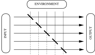
To define our model we need to introduce, for a given integer $n$, a set of $n$ input bosonic oscillators, with canonical variables $\{q_{k},p_{k}\}_{k=1,\dots n}$, and a collection of $n$ ancillary modes, which play the role of the environment, with canonical variables $\{Q_{k},P_{k}\}_{k=1,\dots n}$. In the following we refer to this set of oscillators as the local modes. All the frequencies are assumed to be degenerate and normalized to one. The integer $k$ labels the sequential uses of the channel. At the $k$th use, the $k$th input mode is linearly mixed with the $k$th environment mode at a beam splitter with given transmissivity $\eta$ (see figure 1). In the Heisenberg picture, the channel transforms the input field variables as

$$\begin{array}[]{ccc}q^{\prime}_{k}&=&\sqrt{\eta}\,q_{k}+\sqrt{1-\eta}\,Q_{k}\,,\\ p^{\prime}_{k}&=&\sqrt{\eta}\,p_{k}+\sqrt{1-\eta}\,P_{k}\,.\end{array}$$ (3)

Figure 1: A schematic picture of the model of lossy bosonic channel. Each input mode (left-right line), representing one use of the channel, interacts with the corresponding environment mode (top-bottom line) through a beam-splitter. To introduce memory effects, environment modes are considered in a correlated state.

Memory effects among different uses of the channel are present if the corresponding local modes of the environment are correlated. Here we assume the environment to be in a Gaussian state with zero mean, described by the Wigner function

$$W=\frac{1}{\sqrt{\det(V)}}\exp{\left(-\frac{1}{2}X^{\mathsf{T}}V^{-1}X\right)},$$ (4)

where $X^{\mathsf{T}}:=(Q_{1},Q_{2},\dots Q_{n},P_{1},P_{2},\dots P_{n})$ indicates the vector of coordinates in the environment phase space. The choice of a Gaussian state for the environment makes the channel itself Gaussian. We chose a covariance matrix with the following block-diagonal form

$$V=\frac{1}{2}\left(\begin{array}[]{cc}e^{s\Omega}&\mathbb{O}\\ \mathbb{O}&e^{-s\Omega}\end{array}\right).$$ (7)

This is a bona fide covariance matrix as long as the matrix $\Omega$ is symmetric and the parameter $s$ is real. It represents a multimode squeezed vacuum (see e.g. squeez ). The squeezing parameter $s$ (or $|s|$), determining how strong environment correlations are, can be also interpreted as a measure of memory between different uses of the bosonic channel. As to the form of $\Omega$, we chose the following $n\times n$ matrix:

$$\Omega=\left(\begin{array}[]{cccccc}0&1&0&\dots&0&0\\ 1&0&1&\ddots&0&0\\ 0&1&0&\ddots&0&0\\ \vdots&\vdots&\ddots&\ddots&\vdots&\vdots\\ 0&0&0&\ddots&0&1\\ 0&0&0&\dots&1&0\end{array}\right).$$ (14)

The spectrum of this matrix was already presented in e.g. oleg , its eigenvalues are

$$\lambda_{j}=2\cos{\left(\frac{\pi j}{n+1}\right)}\ \ \mbox{for}\ \ j=1,\dots n,$$ (15)

the components of the corresponding eigenvectors being

$$v_{j,k}=\sqrt{\frac{2}{n+1}}\sin{\left(\frac{jk\pi}{n+1}\right)}\ \ \mbox{for}\ \ k=1,\dots n.$$ (16)

According to Williamson theorem (see e.g. paris ) one can always find a set of collective modes, with canonical variables $\{\tilde{Q}_{j},\tilde{P_{j}}\}_{j=1,\dots n}$, which diagonalize the covariance matrix. In this basis, the Wigner function has the form

$$\tilde{W}=\frac{1}{\sqrt{\det(\tilde{V})}}\exp{\left(-\frac{1}{2}\tilde{X}^{\mathsf{T}}\tilde{V}^{-1}\tilde{X}\right)},$$ (17)

where $\tilde{X}^{\mathsf{T}}:=(\tilde{Q}_{1},\tilde{P}_{1},\dots\tilde{Q}_{n},\tilde{P}_{n})$. An explicit expression for these variables can be obtained from the eigenvectors of the matrix $\Omega$, yielding to define the following variables:

$$\begin{array}[]{ccc}\tilde{Q}_{j}&:=&v_{j,k}Q_{k}\,,\\ \tilde{P}_{j}&:=&v_{j,k}P_{k}\,.\end{array}$$ (20)

Analogously, we introduce the following collective variables at the input field:

$$\begin{array}[]{ccc}\tilde{q}_{j}&:=&v_{j,k}q_{k}\,,\\ \tilde{p}_{j}&:=&v_{j,k}p_{k}\,.\end{array}$$ (23)

We refer to the set of oscillators with field variables $\{\tilde{Q}_{j},\tilde{P}_{j}\}_{j=1,\dots n}$ and $\{\tilde{q}_{j},\tilde{p}_{j}\}_{j=1,\dots n}$ as the collective modes. Let us remark that the action of the channel in the Heisenberg picture on the collective modes is formally unchanged:

$$\begin{array}[]{ccc}\tilde{q}^{\prime}_{j}&=&\sqrt{\eta}\,\tilde{q}_{j}+\sqrt{1-\eta}\,\tilde{Q}_{j}\,,\\ \tilde{p}^{\prime}_{j}&=&\sqrt{\eta}\,\tilde{p}_{j}+\sqrt{1-\eta}\,\tilde{P}_{j}\,.\end{array}$$ (26)

It is worth noticing that the diagonal covariance matrix $\tilde{V}$ is the direct sum of one-mode covariance matrices:

$$\tilde{V}=\bigoplus_{j=1}^{n}\tilde{V}_{j}\,.$$ (27)

That implies that the state of the environment is simply separable in the basis of collective modes. It follows from the transformation (20) that the entries of $\tilde{V}$ are the eigenvalues of $V$. Using the eigenvalues of the matrix $\Omega$, we obtain the following expression for the covariance matrix of the $j$th collective mode:

$$\tilde{V}_{j}=\frac{1}{2}\left(\begin{array}[]{cc}e^{s_{j}}&0\\ 0&e^{-s_{j}}\end{array}\right),$$ (30)

where $s_{j}:=s\lambda_{j}$. We observe that each collective oscillator of the environment is in a squeezed state with $j$ dependent squeezing parameter.

To conclude this section, let us come back to the basis of the local modes. For a given integer $k_{0}\in[1,n]$, by integrating the Wigner function in (4) over the local variables $\{q_{k},p_{k}\}$ for $k\neq k_{0}$ we obtain the Wigner function describing the state of the $k_{0}$th local mode of the environment. The corresponding local state is thermal-like, with average number of excitations:

$$T_{\mathrm{eff}}(s,k_{0})=\frac{1}{2}\left[\sum_{j=1}^{n}v_{j,k_{0}}^{2}e^{s_{j}}\right]-\frac{1}{2}\,.$$ (31)

By the symmetries of $v_{j,k}$ and $s_{j}$, this can be rewritten as follows:

$$T_{\mathrm{eff}}(s,k_{0})=\left\{\begin{array}[]{lr}\left[\sum_{j=1}^{n/2}v_{j,k_{0}}^{2}\cosh{s_{j}}\right]-\frac{1}{2}\,,&\mbox{if $n$ is even.}\\ \left[\sum_{j=1}^{(n-1)/2}v_{j,k_{0}}^{2}\cosh{s_{j}}\right]+\frac{1}{2}v_{(n+1)/2,k_{0}}^{2}-\frac{1}{2}\,,&\mbox{if $n$ is odd}.\end{array}\right.$$ (34)

Notice that the local temperature $T_{\mathrm{eff}}(s,k_{0})$ is a monotonically increasing function of $|s|$.

III Continuous variables encoding/decoding

Classical information is sent via the bosonic channel by choosing a suitable scheme for encoding (by state preparation of the input field) and decoding (by observing the output field) a classical alphabet.

As to the encoding, we introduce a reference pure state of the input field, described by the Gaussian Wigner function

$$w=\frac{1}{\sqrt{\det(\sigma)}}\exp{\left(-\frac{1}{2}x^{\mathsf{T}}\sigma^{-1}x\right)},$$ (35)

expressed in terms of the local variable $x:=(q_{1},\dots q_{n},p_{1},\dots p_{n})^{\mathsf{T}}$. A multivariate Gaussian variable $y:=(y_{q,1},\dots y_{q,n},y_{p,1},\dots y_{p,n})^{\mathsf{T}}$, with probability distribution $P(y)$, zero mean and covariance matrix $Y$, is encoded in the displaced state of the input field described by the Wigner function

$$w_{y}=\frac{1}{\sqrt{\det(\sigma)}}\exp{\left[-\frac{1}{2}(x-y)^{\mathsf{T}}\sigma^{-1}(x-y)\right]}.$$ (36)

Eventually, the state describing the statistical ensemble has the following Wigner function:

$$\bar{w}_{y}=\int w_{y}P(y)\,dy=\frac{1}{\sqrt{\det(\sigma+Y)}}\exp{\left[-\frac{1}{2}x^{\mathsf{T}}(\sigma+Y)^{-1}x\right]}.$$ (37)

To avoid infinite energy we introduce a constraint in the maximum number of excitations at the input field per channel use (i.e. per mode) in average. Allowing no more than $N$ excitations per mode in average, the constraint can be written in terms of the covariance matrices, in natural units:

$$\frac{1}{2n}\mathrm{tr}\left(\sigma+Y\right)\leq N+\frac{1}{2}\,.$$ (38)

We can summarize the action of the channel on Gaussian states as follows. For a given value of the displacement amplitudes (hence for a given letter of the alphabet) the Wigner function at the output field has covariance matrix

$$\sigma^{\prime}_{y}=\eta\sigma+(1-\eta)V.$$ (39)

On the other hand, the output state averaged over the letters of the continuous alphabet has covariance matrix

$$\sigma^{\prime}=\eta(\sigma+Y)+(1-\eta)V.$$ (40)

We can equivalently work in the basis of collective modes, in which the covariance matrix of the reference input state is denoted as $\tilde{\sigma}$. Analogously, the zero mean Gaussian variable $\tilde{y}:=(\tilde{y}_{q,1},\dots\tilde{y}_{p,n})^{\mathsf{T}}$, defined by the relations

$$\begin{array}[]{ccc}\tilde{y}_{q,j}&:=&v_{j,k}y_{q,k}\,,\\ \tilde{y}_{p,j}&:=&v_{j,k}y_{p,k}\,,\end{array}$$ (43)

has covariance matrix $\tilde{Y}$. In the collective basis, the output field is described by the covariance matrices

$$\tilde{\sigma}^{\prime}_{y}=\eta\tilde{\sigma}+(1-\eta)\tilde{V}$$ (44)

and

$$\tilde{\sigma}^{\prime}=\eta(\tilde{\sigma}+\tilde{Y})+(1-\eta)\tilde{V}.$$ (45)

It is worth noticing that the form of the energy constraint is preserved, namely

$$\frac{1}{2n}\mathrm{tr}\left(\tilde{\sigma}+\tilde{Y}\right)\leq N+\frac{1}{2}\,.$$ (46)

Homodyne detection requires the choice of a compatible set of $n$ quadratures to be measured at the output field. A generic set of quadratures is

$$\{z_{h}\ \ |\ \ z_{h}=\mathbb{R}_{hk}q_{k}+\mathbb{S}_{hk}p_{k}\}$$ (47)

for any pair of $n\times n$ matrices $\mathbb{R}$, $\mathbb{S}$ satisfying the relations $\mathbb{R}\mathbb{R}^{\mathsf{T}}+\mathbb{S}\mathbb{S}^{\mathsf{T}}=\mathbb{I}$ and $\mathbb{R}\mathbb{S}^{\mathsf{T}}-\mathbb{S}\mathbb{R}^{\mathsf{T}}=\mathbb{O}$ (see e.g. paris ). Assuming ideal homodyne, the distribution of the stochastic variable $z:=(z_{1},\dots z_{n})^{\mathsf{T}}$ is Gaussian with zero mean. Its covariance matrix, which we denote as $Z$, can be computed from the output field covariance matrix using the relations in (47).

For given covariance matrices $V$, $\sigma$, and for a given set of quadratures to be measured, a classical channel is defined from the quantum one. The capacity of the classical channel can be computed as the maximum of the mutual information between the output and the input variables:

$$I(z;y)=H(z)-H(z|y),$$ (48)

where $H$ denotes the Shannon entropy. The maximization has to be taken over all possible expressions of the covariance matrix $Y$ compatible with the energy constraint.

IV Achievable bit rates with homodyne detection

Let us now consider the form of the Wigner function for the reference input state, determined by the covariance matrix $\sigma$, and the form of the distribution of the classical variable $y$, determined by the covariance matrix $Y$. Here we distinguish and compare two cases: the first one corresponds to a local encoding in which $\sigma$ and $Y$ are diagonal; the second one is a collective encoding in which $\tilde{\sigma}$ and $\tilde{Y}$ are diagonal. From the view point of the local modes, in the local encoding scheme information is always carried by simply separable (unentangled) states, while the collective encoding deals with states which are in general entangled.

Let us first describe the case of local encoding. In the basis of the local modes, the diagonal $\sigma$ can be parameterized as follows

$$\sigma=\bigoplus_{k=1}^{n}\sigma_{k}.$$ (49)

We introduce the real parameters $\{r_{k}\}$, such that

$$\sigma_{k}=\left(\begin{array}[]{cc}\langle q_{k}^{2}\rangle&\frac{1}{2}\langle q_{k}p_{k}+p_{k}q_{k}\rangle\\ \frac{1}{2}\langle q_{k}p_{k}+p_{k}q_{k}\rangle&\langle p_{k}^{2}\rangle\end{array}\right)=\frac{1}{2}\left(\begin{array}[]{cc}e^{r_{k}}&0\\ 0&e^{-r_{k}}\end{array}\right).$$ (54)

Analogously, the covariance matrix $Y$ reads

$$Y=\bigoplus_{k=1}^{n}Y_{k}$$ (55)

and is parameterized by the positive parameters $\{c_{q,k},c_{p,k}\}$:

$$Y_{k}=\frac{1}{2}\left(\begin{array}[]{cc}c_{q,k}&0\\ 0&c_{p,k}\end{array}\right).$$ (58)

As to the decoding part, the natural choice is to measure the local quadratures

$$z_{k}:=\cos{\theta_{k}}q_{k}+\sin{\theta_{k}}p_{k}\,.$$ (59)

The covariance matrix of the output variable $z:=(z_{1},\dots z_{n})^{\mathsf{T}}$ can be easily computed. It is diagonal as well, with the variances:

$$\langle z_{k}^{2}\rangle=\cos^{2}{\theta_{k}}\left[\eta\left(\frac{e^{r_{k}}}{2}+c_{q,k}\right)+(1-\eta)\left(T_{\mathrm{eff}}(s,k)+\frac{1}{2}\right)\right]+\sin^{2}{\theta_{k}}\left[\eta\left(\frac{e^{-r_{k}}}{2}+c_{p,k}\right)+(1-\eta)\left(T_{\mathrm{eff}}(s,k)+\frac{1}{2}\right)\right].$$ (60)

The output variable has conditioned covariance matrix, denoted $Z_{y}$, which is diagonal with entries

$$\langle z_{k}^{2}\rangle_{y}=\cos^{2}{\theta_{k}}\left[\eta\frac{e^{r_{k}}}{2}+(1-\eta)\left(T_{\mathrm{eff}}(s,k)+\frac{1}{2}\right)\right]+\sin^{2}{\theta_{k}}\left[\eta\frac{e^{-r_{k}}}{2}+(1-\eta)\left(T_{\mathrm{eff}}(s,k)+\frac{1}{2}\right)\right].$$ (61)

Since all the probability distributions are Gaussian, the mutual information can be easily written in terms of the covariance matrices:

$$I(z;y)=\frac{1}{2}\log_{2}{\left[\det(Z)\right]}-\frac{1}{2}\log_{2}{\left[\det(Z_{y})\right]}=\frac{1}{2}\sum_{k=1}^{n}\log_{2}{\left(\frac{\langle z_{k}^{2}\rangle}{\langle z_{k}^{2}\rangle_{y}}\right)}.$$ (62)

The maximization of the mutual information is over the $3n$ parameters $r_{k},c_{q,k},c_{p,k}$ satisfying the constraints

$$\frac{1}{2n}\sum_{k=1}^{n}\left(\cosh{r_{k}}+c_{q,k}+c_{p,k}\right) = N_{k}+\frac{1}{2}\,,$$ (63)

$$\frac{1}{n}\sum_{k=1}^{n}N_{k}\leq N,$$ (64)

and over the $n$ angles $\theta_{k}$, which determine the chosen quadratures. Concerning the choice of the optimal quadratures, it is immediate to recognize that the maximum is reached for $\sin{\theta_{k}}=0$ if $r_{k}>0$, and for $\cos{\theta_{k}}=0$ if $r_{k}<0$, while the value of $\theta_{k}$ is irrelevant if $r_{k}=0$. Maximizing over the remaining variables and applying the additivity of mutual information, we obtain the following expression for the maximum mutual information with local encoding/decoding scheme:

$$F_{\mathrm{loc}}=\max_{\{N_{k}\}}\left\{\frac{1}{2}\sum_{k=1}^{n}\log_{2}{\left[1+2\frac{2N_{k}+1-\cosh{r_{k}^{\mathrm{opt}}}}{e^{-r_{k}^{\mathrm{opt}}}+\nu(2T_{\mathrm{eff}}(s,k)+1)}\right]}\ \ |\ \ \frac{1}{n}\sum_{k=1}^{n}N_{k}\leq N\right\},$$ (65)

where

$$e^{r_{k}^{\mathrm{opt}}}=\frac{1}{\nu(2T_{\mathrm{eff}}(s,k)+1)}\left[\sqrt{1+\nu(2T_{\mathrm{eff}}(s,k)+1)\left(\nu(2T_{\mathrm{eff}}(s,k)+1)+4N_{k}+2\right)}-1\right],$$ (66)

and we have defined $\nu:=(1-\eta)/\eta$.

Let us now consider the case of collective encoding. In the basis of the collective modes, the diagonal $\tilde{\sigma}$ can be parameterized as follows

$$\tilde{\sigma}=\bigoplus_{j=1}^{n}\tilde{\sigma}_{j}$$ (67)

with

$$\tilde{\sigma}_{j}=\frac{1}{2}\left(\begin{array}[]{cc}e^{\tilde{r}_{j}}&0\\ 0&e^{-\tilde{r}_{j}}\end{array}\right).$$ (70)

Analogously, the covariance matrix $\tilde{Y}$ is

$$\tilde{Y}=\bigoplus_{j=1}^{n}\tilde{Y}_{j}$$ (71)

with

$$\tilde{Y}_{j}=\frac{1}{2}\left(\begin{array}[]{cc}\tilde{c}_{q,j}&0\\ 0&\tilde{c}_{p,j}\end{array}\right).$$ (74)

As to the decoding part, the natural choice is to measure the collective quadratures defined as

$$\tilde{z}_{j}=\cos{\theta_{j}}\tilde{q}_{j}+\sin{\theta_{j}}\tilde{p}_{j}\,.$$ (75)

The output variable $\tilde{z}:=(\tilde{z}_{1},\dots\tilde{z}_{n})^{\mathsf{T}}$ has diagonal covariance matrix $\tilde{Z}$ and conditional covariance matrix $\tilde{Z}_{y}$. The corresponding variances read

$$\langle\tilde{z}_{j}^{2}\rangle=\cos^{2}{\theta_{j}}\left[\eta\left(\frac{e^{\tilde{r}_{j}}}{2}+\tilde{c}_{q,j}\right)+(1-\eta)\frac{e^{s_{j}}}{2}\right]+\sin^{2}{\theta_{j}}\left[\eta\left(\frac{e^{-\tilde{r}_{j}}}{2}+\tilde{c}_{p,j}\right)+(1-\eta)\frac{e^{-s_{j}}}{2}\right]$$ (76)

and

$$\langle\tilde{z}_{j}^{2}\rangle_{y}=\cos^{2}{\theta_{j}}\left[\eta\frac{e^{\tilde{r}_{j}}}{2}+(1-\eta)\frac{e^{s_{j}}}{2}\right]+\sin^{2}{\theta_{j}}\left[\eta\frac{e^{-\tilde{r}_{j}}}{2}+(1-\eta)\frac{e^{-s_{j}}}{2}\right].$$ (77)

It is easy to recognize that the maximum of the mutual information is reached for $\sin{\theta_{j}}=0$ if $s_{j}>0$, and for $\cos{\theta_{j}}=0$ if $s_{j}<0$, finally if $s_{j}=0$ we can argue as in the case of local encoding. By maximizing over the remaining $3n$ variables $\{\tilde{r}_{j}$, $\tilde{c}_{q,j}$, $\tilde{c}_{p,j}\}$ under the constraints

$$\frac{1}{2n}\sum_{j=1}^{n}\left(\cosh{\tilde{r}_{j}}+\tilde{c}_{q,j}+\tilde{c}_{p,j}\right) = N_{j}+\frac{1}{2}\,,$$ (78)

$$\frac{1}{n}\sum_{j=1}^{n}N_{j}\leq N$$ (79)

and applying the additivity of the mutual information, we obtain the following expression for the maximum rate of transmission with encoding/decoding in collective variables:

$$F_{\mathrm{coll}}=\max_{\{N_{j}\}}\left\{\frac{1}{2}\sum_{j=1}^{n}\log_{2}{\left[1+2\frac{2N_{j}+1-\cosh{\tilde{r}_{j}^{\mathrm{opt}}}}{e^{-\tilde{r}_{j}^{\mathrm{opt}}}+\nu e^{-|s_{j}|}}\right]}\ \ |\ \ \frac{1}{n}\sum_{j=1}^{n}N_{j}\leq N\right\}.$$ (80)

The optimal value $\tilde{r}_{j}^{\mathrm{opt}}$ is determined by the equation

$$e^{\tilde{r}_{j}^{\mathrm{opt}}}=\frac{e^{|s_{j}|}}{\nu}\left[\sqrt{1+\nu e^{-|s_{j}|}\left(\nu e^{-|s_{j}|}+4N_{j}+2\right)}-1\right].$$ (81)

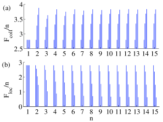
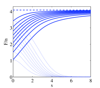
The maximum mutual informations per channel use, respectively defined as $F_{\mathrm{loc}}/n$ and $F_{\mathrm{coll}}/n$, are plotted in figure 2 as function of number of uses of the channel, for several values of the memory parameter. The case $n=1$ or $s=0$ correspond to the memoryless channel. Notice the different behavior of the rates as the number of uses (or the value of the memory parameter) increases. The same quantities are plotted together in figure 3, for $n=10$ uses of the channel, as function of the memory parameter, for several values of the beam splitter transmissivity. Notice the different behavior of the rates corresponding to local (dotted line) and collective (solid line) encoding/decoding scheme.

Figure 2: The histograms show the maximum achievable rates per channel use with collective (a) and local (b) encoding/decoding scheme, as function of the number of channel uses. For each value of $n$, the histograms correspond to different values of the memory parameter, from the left to the right $s=0$, $s=1$, $s=2$, $s=3$. The maximum average excitations per mode is $N=8$, the transmissivity $\eta=0.7$.

Figure 3: The plot shows the achievable rates per channel use with collective (solid line) and local (dotted line) encoding/decoding scheme, as function of the memory parameter, for $n=10$ uses of the channel. The curves correspond to different values of the transmissivity, from the bottom to the top $\eta$ varies from $\eta=0.1$ to $\eta=0.9$ by steps of $0.1$. The maximum average excitations per mode is $N=8$, which corresponds to the asymptotic value (plotted in dashed line) of the rate with collective scheme (see equation (83)): $\lim_{s\rightarrow\infty}F_{\mathrm{coll}}/n=\log_{2}(2N+1)\simeq 4.0875$.

The expression of the maximal mutual information allows to make comparison with the memoryless case (see also the plot in figure 3). First of all, let us recall that the memoryless channel is recovered for $s=0$; our results show that the maximum mutual information is a monotonically increasing function of $|s|$ in the case of collective encoding/decoding scheme, while it is monotonically decreasing in the case of the local one. This is enough to conclude that, in the presence of memory, collective encoding/decoding is the optimal choice. Secondly, let us notice that the two schemes are equivalent in the memoryless case, i.e. $s=0$ or $n=1$; that leads to conclude that the presence of memory enhances the bit rate as long as collective encoding/decoding is allowed.

V Conclusion

We have discussed the model of lossy bosonic Gaussian channel with memory presented in oleg , an instance of a general class of bosonic memory channel introduced in mancini . Our model is characterized by a single parameter which determines the amount of memory contained in the channel. By considering the case of homodyne detection, we have compared two different encoding/decoding schemes: a local one in which classical information is encoded and carried by unentangled (simply separable) states; and a collective scheme based on states which are in general entangled among different uses of the channel. We have computed the maximum achievable bit rate using both the schemes, assuming energy constrains at the input field, for an arbitrary number of channel uses. Our results lead to conclude that, as the memory parameter increases, the collective scheme becomes more and more efficient than the local one. It is hence interesting to analyze the asymptotic limit of the rates for $|s|\rightarrow\infty$, corresponding to infinite memory. From the expressions in (65) and (80) we obtain

$$\lim_{s\rightarrow\infty}\frac{F_{\mathrm{loc}}}{n}=0$$ (82)

and

$$\lim_{s\rightarrow\infty}\frac{F_{\mathrm{coll}}}{n}=\log_{2}{(2N+1)}.$$ (83)

Notice that the latter expression holds independently of $n$ and for any value of $\eta\neq 0,1$. Interestingly enough, the asymptotic value in (83) equals the maximum achievable rate of the (memoryless) noiseless channel ($\eta=1$) with homodyne detection (see holevo1 ). In this sense, by using local encoding/decoding one sees infinite noise in the channel with high degree of memory, while by using a collective encoding/decoding one can completely avoid it.

References

• (1) D. Kretschmann and R. F. Werner, Phys. Rev. A 72, 062323 (2005).
• (2) C. Macchiavello, and G. M. Palma, Phys. Rev. A 65, 050301(R) (2002);
C. Macchiavello, G. M. Palma, and S. Virmani, Phys. Rev. A 69, 010303(R) (2004);
D. Daems, Phys. Rev. A 76, 012310 (2007).
• (3) N. J. Cerf, J. Clavareau, C. Macchiavello, and J. Roland, Phys. Rev. A 72, 042330 (2005);
N. Cerf, J. Clavareau, J. Roland, and C. Macchiavello, e-print arXiv:quant-ph/0508197.
• (4) A. S. Holevo, M. Soma and O. Hirota, Phys. Rev. A 59, 1820 (1999).
• (5) A. S. Holevo and R. F. Werner, Phys. Rev. A 63, 032312 (2001).
• (6) O. V. Pilyavets, V. G. Zborovskii and S. Mancini, Phys. Rev. A 77, 052324 (2008).
• (7) V. Giovannetti and S. Mancini, Phys. Rev. A 71, 062304 (2005).
• (8) G. Ruggeri, G. Soliani, V. Giovannetti, and S. Mancini, Europhys. Lett. 70, 719 (2005);
G. Ruggeri and S. Mancini, Phys. Lett. A 362, 340 (2007).
• (9) C. F. Lo and R. Sollie, Phys. Rev. A 47, 733 (1993).
• (10) A. Ferraro, S. Olivares and M. G. A. Paris, Gaussian states in quantum information (Bibliopolis, Napoli, 2005), e-print arXiv:quant-ph/0503237.