PSI-PR-09-01

Chiral expansions of the $\pi^{0}$ lifetime

K. Kampf ^1,2 and B. Moussallam³

¹ Paul Scherrer Institut, Ch-5232 Villigen PSI, Switzerland

² IPNP, Charles University, Faculty of Mathematics and Physics
V Holešovičkách 2, CZ-180 00 Prague 8, Czech Republic

³ Groupe de Physique Théorique, Institut de Physique Nucléaire
Université Paris-Sud 11, F-91406 Orsay, France

Abstract

The corrections induced by light quark masses to the current algebra result for the $\pi^{0}$ lifetime are reexamined. We consider next-to-next-to-leading order corrections and we compute all the one-loop and the two-loop diagrams which contribute to the decay amplitude at this order in the two-flavour chiral expansion. We show that the result is renormalizable, as Weinberg consistency conditions are satisfied. We find that chiral logarithms are present at this order unlike the case at next-to-leading order. The result could be used in conjunction with lattice QCD simulations, the feasibility of which was recently demonstrated. We discuss the matching between the two-flavour and the three-flavour chiral expansions in the anomalous sector at order one-loop and derive the relations between the coupling constants. A modified chiral counting is proposed, in which $m_{s}$ counts as $O(p)$. We have updated the various inputs needed and used this to make a phenomenological prediction.

1 Introduction

The close agreement between the current algebra prediction for the lifetime of the neutral pion and experiment is one of the two compelling experimental signatures, together with the Nambu-Goldberger-Treiman relation, for the spontaneous breaking of chiral symmetry in QCD. There is an ongoing effort by the PrimEx collaboration [1] to improve significantly the accuracy of the lifetime measurement, which is now around 8%, down to the 1%-2% level. This motivates us to study the corrections to the current algebra prediction.

Starting with the detailed study by Kitazawa [2], this problem has been addressed several times in the literature [3, 4, 5, 6, 7, 8, 9, 10, 11]. The approach used in ref. [2] was to extrapolate from the soft pion limit to the physical pion mass result using the Pagels-Zepeda [12] sum rule method. This was reconsidered in ref. [10] who implemented a more elaborate treatment of $\pi^{0}-\eta-\eta^{\prime}$ mixing and also recently in ref. [11]. The latter work shows some disagreement concerning the size of the $\eta^{\prime}$ meson contribution in the sum rule as compared to earlier results.

In this paper, we reconsider the issue of the corrections to the current algebra result to the $\pi^{0}\to 2\gamma$ amplitude from the point of view of a strict expansion as a function of the light quark masses. This is most easily implemented by using chiral Lagrangian methods (see e.g. [13] for a review). The same framework also allows one to compute radiative corrections [14]. We believe that it is somewhat easier to control the size of the errors in this kind of approach, which is important for exploiting the forthcoming high experimental accuracy. Another interest in deriving a quark mass expansion is the ability to perform comparisons with lattice QCD results where quark masses can be varied. The feasibility of computing the $\pi^{0}$ to two photon amplitude in lattice QCD has been studied very recently [15].

A priory, it is expected that one can make use of $SU(2)$ ChPT, i.e. expand as a function of $m_{u}$, $m_{d}$ without making any assumption concerning $m_{s}$ (except that it is heavier than $m_{u}$, $m_{d}$). In $SU(2)$ ChPT it is often the case that chiral logarithms provide a reasonable order of magnitude for the size of the chiral corrections. This is the case, for instance, for the $\pi\pi$ scattering amplitude [16, 17]. It was observed in refs. [3, 4] that there was no chiral logarithm in the next-to-leading order (NLO) correction to the $\pi^{0}$ lifetime once the amplitude is expressed in terms of the physical value of $F_{\pi}$. We have asked ourselves whether chiral logarithms are present in the NNLO corrections. At this order, the coefficient of the double chiral logarithm depends only on $F_{\pi}$. Depending on its numerical coefficient, such a term could modify the NLO results. In order to obtain this coefficient it is, in principle, sufficient to compute a set of one-loop graphs containing one divergent NLO vertex [18]. For completeness, we will perform a complete calculation of the two-loop graphs as well. This is described in sec. 3.

In the framework of two-flavour ChPT, however, one faces the practical problem that the polynomial terms in $m_{u},\ m_{d}$ at NLO involve a number of low-energy couplings (LEC’s) which are not known. We will show that it is possible to make estimates for the relevant combinations, and then make quantitative predictions for the $\pi^{0}$ decay, under the minimal additional assumption that the mass of the strange quark is sufficiently small, justifying a chiral expansion in $m_{s}$. We will obtain the first two terms in the $m_{s}$ expansion of the NLO $SU(2)$ LEC’s. The result can be implemented in association with a modified chiral counting scheme, in which $m_{s}$ is counted as $O(p)$, which respects the hierarchy $m_{u},\ m_{d}\ll m_{s}$. This leads to simpler formulas than previously obtained. Finally, we will update all the inputs needed to compute the lifetime.

2 Leading and next-to-leading orders in the $SU(2)$ expansion

In the odd-intrinsic-parity sector, the Lagrangian of lowest chiral order has order $p^{4}$, it is the Wess-Zumino [19] Lagrangian, ${\cal L}^{WZ}$, which form is dictated by the ABJ anomaly [20]. Writing the $\pi^{0}\to\gamma(k_{1})\gamma(k_{2})$ decay amplitude in the form

$${\cal T}=e^{2}\epsilon(e_{1}^{*},k_{1},e_{2}^{*},k_{2})T\ ,$$ (1)

a tree level computation of the pion decay amplitude gives the well known result

$$T_{LO}={1\over 4\pi^{2}F}\ ,$$ (2)

where $F$ is the pion decay constant in the two-flavour chiral limit $m_{u}=m_{d}=0$. At leading order one can set $F=F_{\pi}$ in eq. (2). According to the Weinberg rules[18] for ChPT, the NLO corrections are generated from:

• One-loop diagrams with one vertex taken from ${\cal L}^{WZ}$ and other vertices from the $O(p^{2})$ chiral Lagrangian. These diagrams were first computed in refs. [3, 4].

• Tree diagrams having one vertex from ${\cal L}^{WZ}$ and one vertex from the $O(p^{4})$ chiral Lagrangian.

• Tree diagrams from the $O(p^{6})$ Lagrangian in the anomalous-parity sector, ${\cal L}^{W}_{(6)}$.

The classification of a minimal set of independent terms in this Lagrangian was initiated in refs. [21, 22]. We will use here the result of ref. [23] who further reduced the set to 23 terms in the case of three flavours and to 13 independent terms in the case of two flavours (this result was also obtained in ref. [24]). The list, in the case of two flavours, is recalled below:

$${\cal L}^{W}_{6,N_{f}=2}=\epsilon^{\alpha\beta\mu\nu}\Big{\{}\; c^{W}_{1}{\langle\chi_{+}{[f_{-\mu\nu},u_{\alpha}u_{\beta}]}\rangle} + c^{W}_{2}{\langle\chi_{-}{\{f_{+\mu\nu},u_{\alpha}u_{\beta}\}}\rangle} + c^{W}_{3}i{\langle\chi_{-}f_{+\mu\nu}f_{+\alpha\beta}\rangle}$$

$$+ c^{W}_{4}i{\langle\chi_{-}f_{-\mu\nu}f_{-\alpha\beta}\rangle} + c^{W}_{5}i{\langle\chi_{+}{[f_{+\mu\nu},f_{-\alpha\beta}]}\rangle} + c^{W}_{6}{\langle f_{+\mu\nu}\rangle}{\langle\chi_{-}u_{\alpha}u_{\beta}\rangle}$$

$$+ c^{W}_{7}i{\langle f_{+\mu\nu}\rangle}{\langle f_{+\alpha\beta}\chi_{-}\rangle} + c^{W}_{8}i{\langle f_{+\mu\nu}\rangle}{\langle f_{+\alpha\beta}\rangle}{\langle\chi_{-}\rangle} + c^{W}_{9}i{\langle f_{+\gamma\mu}\rangle}{\langle h^{\gamma}_{\>\nu}u_{\alpha}u_{\beta}\rangle}$$

$$+ c^{W}_{10}i{\langle f^{\,\gamma}_{+\ \mu}\rangle}{\langle f_{-\gamma\nu}u_{\alpha}u_{\beta}\rangle} + c^{W}_{11}{\langle f_{+\mu\nu}\rangle}{\langle f_{+\gamma\alpha}h^{\gamma}_{\>\beta}\rangle} + c^{W}_{12}{\langle f_{+\mu\nu}\rangle}{\langle f^{\,\gamma}_{+\ \alpha}f_{-\gamma\beta}\rangle}$$

$$+ c^{W}_{13}{\langle\nabla^{\gamma}f_{+\gamma\mu}\rangle}{\langle f_{+\nu\alpha}u_{\beta}\rangle} \Big{\}}\ .$$ (3)

The relations between the bare and the renormalized couplings may be written as [23]

$$c^{W}_{i}=c_{i}^{Wr}(\mu)+\eta_{i}^{W}{(c\mu)^{d-4}\over 16\pi^{2}(d-4)}$$ (4)

with $\log(c)=-(\log(4\pi)-\gamma+1)/2$ as usual in ChPT (note that the couplings $c^{Wr}_{i}$ have dimension $(mass)^{-2}$). The coefficients $\eta_{i}^{W}$ vanish for $i=1...5$ and the remaining ones read [23]

$$\begin{array}[]{llll}\eta_{6}^{W}=3\alpha,&\eta_{7}^{W}=3\alpha,&\eta_{8}^{W}=-{3\over 2}\alpha,&\eta_{9}^{W}=6\alpha\\[5.69046pt] \eta_{10}^{W}=-18\alpha,&\eta_{11}^{W}=12\alpha,&\eta_{12}^{W}=0,&\eta_{13}^{W}=-12\alpha\ ,\end{array}$$ (5)

with

$$\alpha=1/(384\pi^{2}F^{2})\ .$$ (6)

The above results for $\eta_{i}^{W}$ were obtained by using, in the ordinary sector at $p^{4}$, the chiral Lagrangian term proportional to $l_{4}$ which differs from the form originally used in ref. [25]

$${\cal L}_{l_{4}}^{({\rm orig})}={il_{4}\over 4}{\langle u^{\mu}\chi_{\mu-}\rangle}$$ (7)

by a term proportional to the equation of motion

$${\cal L}_{l_{4}}={\cal L}_{l_{4}}^{({\rm orig})}+{il_{4}\over 4}{\langle\hat{\chi}_{-}(\nabla_{\mu}u^{\mu}-{i\over 2}\hat{\chi}_{-})\rangle}\ .$$ (8)

If one uses ${\cal L}_{l_{4}}^{({\rm orig})}$ then, in the odd-intrinsic-parity sector, the coefficients with labels 6,7 and 8 are modified to $\tilde{c}_{i}^{W}$ [26, 7]. The relations between $\tilde{c}_{i}^{W}$ and $c^{W}_{i}$ are easily worked out by performing a field redefinition,

$$\tilde{c}_{6}^{W}=c_{6}^{W}-{N_{c}\over 128\pi^{2}}{l_{4}\over F^{2}}$$

$$\tilde{c}_{7}^{W}=c_{7}^{W}+{N_{c}\over 256\pi^{2}}{l_{4}\over F^{2}}$$

$$\tilde{c}_{8}^{W}=c_{8}^{W}-{N_{c}\over 512\pi^{2}}{l_{4}\over F^{2}}\ .$$ (9)

In the present work, we use the original ${\cal L}_{l_{4}}^{({\rm orig})}$ in our calculations but we will express the final result in terms of $c^{Wr}_{i}$ rather than $\tilde{c}_{i}^{Wr}$, making use of the relations (2) (which will prove slightly more convenient below when we perform a matching with the $SU(3)$ expansion).

Returning to the $\pi^{0}$ decay amplitude, the contributions from the one-loop Feynman diagrams can be shown to be absorbed into the re-expression of $F$ into $F_{\pi}$ [4, 3], the physical pion decay constant at order $p^{4}$, such that the decay amplitude including the NLO corrections reads

$$T_{LO+NLO}={1\over F_{\pi}}\Bigg{\{}{1\over 4\pi^{2}}+{16\over 3}{m_{\pi}^{2}}\left(-4c^{Wr}_{3}-4c^{Wr}_{7}+c^{Wr}_{11}\right)$$

$$\phantom{T_{NLO}=e^{2}\Big{\{}4\pi}+{64\over 9}{B(m_{d}-m_{u})}(5c^{Wr}_{3}+c^{Wr}_{7}+2c^{Wr}_{8})\Bigg{\}}\ ,$$ (10)

where $B=-\lim_{m_{u}=m_{d}=0}{\langle\bar{u}u\rangle}/F^{2}$ and $m_{\pi}^{2}$ denotes the mass squared of the neutral pion which, at this order, is equal to $M^{2}=B(m_{d}+m_{u})$ . Eq. (2) shows that the decay amplitude at NLO receives a contribution proportional to the isospin breaking mass difference $m_{d}-m_{u}$. As can be seen from eqs. (5) the two combinations of chiral couplings which enter into the expression of $T_{NLO}$ are finite. The expression of $T_{LO+NLO}$ therefore involves no chiral logarithm. The chiral corrections to the current algebra result are purely polynomial in $m_{u},\ m_{d}$ and are controlled by four coupling constants from eq. (3). In order to estimate quantitatively the effects of the NLO corrections, we will show below that it is useful to express these couplings as an expansion in powers of the strange quark mass. Before doing so, let us now investigate the presence of chiral logarithms, which could possibly be numerically important, in the NNLO corrections.

3 $\pi^{0}$ decay to NNLO in the two-flavour expansion

We must calculate now a) the one-loop Feynman diagrams with one vertex involving an NLO chiral coupling, either $l_{i}$ or $c_{i}^{W}$ and b) the two-loop Feynman diagrams with one vertex taken from the LO Wess-Zumino Lagrangian and the other one taken from the $O(p^{2})$ chiral Lagrangian. It is convenient the use the following representation for the chiral field

$$U=\sigma+i{\vec{\tau}\cdot\vec{\pi}\over F},\quad\sigma=\sqrt{1-{\vec{\pi}^{2}\over F^{2}}}$$ (11)

(since, in this representation, there is no $\gamma 4\pi$ vertex at LO). At the order considered, all the reducible diagrams are generated from wave-function renormalization. The expression for the WF renormalization constant $Z$ (corresponding to (11)) was first given by Bürgi [27],

$$Z^{1\over 2}=1-{T_{M}\over 2F^{2}}+{1\over F^{4}}\Bigg{[}-{1\over 8}T_{M}^{2}+{M^{4}\over 2}\left(r_{Z}+\dot{T}_{M}^{2}Q^{Z}-\dot{T}_{M}\sum_{i=1}^{3}l_{i}Q_{i}^{Z}\right)$$

$$\phantom{Z^{1\over 2}=1-{T_{M}\over 2F^{2}}}+{B^{2}(m_{d}-m_{u})^{2}}\left(-8F^{2}(c_{7}+c_{9})+\dot{T}_{M}l_{7}\right)\Bigg{]}$$ (12)

with

$$T_{M}={(M^{2})^{{d\over 2}-1}\Gamma(1-{d\over 2})\over(4\pi)^{d\over 2}},\ \dot{T}_{M}={dT_{M}\over dM^{2}},\ d=4+2w\ .$$ (13)

We have indicated explicitly here the contributions proportional to $(m_{d}-m_{u})^{2}$ for completeness because isospin breaking contributions play an important role for the $\pi^{0}$ decay amplitude. We will also need the expression for the chiral expansion of $F_{\pi}$ at order $p^{6}$ (from [28])

$${F_{\pi}\over F}=1+{1\over F^{2}}[M^{2}l_{4}-T_{M}]+{M^{4}\over F^{4}}\left[r_{F}+\dot{T}_{M}^{2}Q^{F}-\dot{T}_{M}\sum_{i=1}^{4}l_{i}Q_{i}^{F}\right]+{8B^{2}(m_{d}-m_{u})^{2}\over F^{2}}(c_{7}+c_{9})\ .$$ (14)

The numerical parameters $Q^{Z}$ and $Q^{F}$ which appear above read

$$Q^{Z}={1\over 96}(96-464w+1185w^{2}),\quad Q^{F}=-{1\over 192}(240-656w+1125w^{2})$$ (15)

and will need the following relations obeyed by the numerical parameters $Q_{i}^{Z}$ and $Q_{i}^{F}$

$$Q_{1}^{F}={-1\over 2}Q_{1}^{Z}\quad Q_{2}^{F}={-1\over 2}Q_{2}^{Z},\quad Q_{3}^{F}=Q_{3}^{Z}=2,\quad Q_{4}^{F}={1\over 2(1+w)}\ .$$ (16)

Finally, the entries $r_{Z}$ and $r_{F}$ in eqs. (3), (14) represent combinations of coupling constants from the $O(p^{6})$ chiral Lagrangian. The $\pi^{0}$ amplitude involves the combination $r_{Z}+2r_{F}$ which is expressed in terms of a single $p^{6}$ coupling, called $c_{6}$ in the classification of ref. [29]

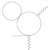
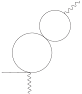
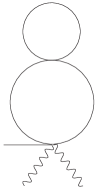
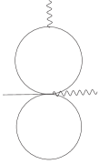
(a)	(b)	(c)	(d)
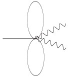
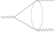
(e)	(f)	(g)

Figure 1: Two-loop Feynman graphs (one-particule irreducible) contributions to the $\pi^{0}\to 2\gamma$ amplitude.

$$r_{Z}+2r_{F}=-64F^{2}\,c_{6}\ .$$ (17)

The two-loop one-particle irreducible diagrams which one must compute (using the representation (11)) are shown in fig. 1. It turns out to be possible to express all of them analytically in terms of known special functions by combining the methods exposed in ref. [30] with integration by parts methods. We give the results corresponding to the two diagrams (f) and (g), which are the most difficult ones, in appendix 1.

Collecting all the pieces together, we find that the expression for the NNLO contribution to the $\pi^{0}$ decay amplitude into two photons has the following expression,

$$F_{\pi}\,T_{NNLO}=-{M^{4}\over 24\pi^{2}F^{4}}\,\left({1\over 16\pi^{2}}L_{\pi}\right)^{2}$$

$$+{M^{4}\over 16\pi^{2}F^{4}}\,L_{\pi}\left[{3\over 256\pi^{4}}+{32F^{2}\over 3}\left(2c^{Wr}_{2}+4c^{Wr}_{3}+2c^{Wr}_{6}+4c^{Wr}_{7}-c^{Wr}_{11}\right)\right]$$

$$+{32M^{2}B(m_{d}-m_{u})\over 48\pi^{2}F^{4}}\,L_{\pi}\,\left[-6c^{Wr}_{2}-11c^{Wr}_{3}+6c^{Wr}_{4}-12c^{Wr}_{5}-c^{Wr}_{7}-2c^{Wr}_{8}\right]$$

$$+{M^{4}\over F^{4}}\lambda_{+}+{M^{2}B(m_{d}-m_{u})\over F^{4}}\lambda_{-}+{B^{2}(m_{d}-m_{u})^{2}\over F^{4}}\lambda_{--}\ ,$$ (18)

where $L_{\pi}$ represents the chiral logarithm

$$L_{\pi}=\log{m_{\pi}^{2}\over\mu^{2}}$$ (19)

and $\lambda_{+}$, $\lambda_{-}$, $\lambda_{--}$ can be expressed as follows in terms of renormalized chiral coupling constants,

$$\lambda_{+}={1\over\pi^{2}}\left[-{2\over 3}d_{+}^{Wr}(\mu)-8c_{6}^{r}-{1\over 4}(l_{4}^{r})^{2}+{1\over 512\pi^{4}}\left(-{983\over 288}-{4\over 3}\zeta(3)+3\sqrt{3}\,{\rm Cl}_{2}(\pi/3)\right)\right]$$

$$\phantom{\lambda_{+}=}+{16\over 3}F^{2}\left[\,8l_{3}^{r}(c^{Wr}_{3}+c^{Wr}_{7})+l_{4}^{r}(-4c^{Wr}_{3}-4c^{Wr}_{7}+c^{Wr}_{11})\right]$$

$$\lambda_{-}={64\over 9}\left[d_{-}^{Wr}(\mu)+F^{2}l_{4}^{r}\,(5c^{Wr}_{3}+c^{Wr}_{7}+2c^{Wr}_{8})\right]$$

$$\lambda_{--}=d_{--}^{Wr}(\mu)-128F^{2}l_{7}(c^{Wr}_{3}+c^{Wr}_{7})\ .$$ (20)

Here, the notation $d^{Wr}$ refer to combinations of couplings from the NNLO Lagrangian (i.e. of order $p^{8}$) in the anomalous sector.

A few remarks are in order concerning this calculation. First, concerning non-local divergences, i.e. terms of the form $M^{4}\log(M^{2})/(d-4)$, we have verified that those which are generated from the two-loop diagrams are cancelled exactly by those generated from the one-loop diagrams proportional to $l_{i}$, $c_{i}^{W}$ as expected from the Weinberg consistency conditions. The divergences that are left are proportional to $M^{4}$, $M^{2}(m_{d}-m_{u})$ and $(m_{d}-m_{u})^{2}$. They are cancelled by the contributions, at tree level, from the chiral Lagrangian of order $p^{8}$ in the anomalous sector. We have denoted the three independent combinations of $O(p^{8})$ chiral couplings by $d_{+}^{W}$, $d_{-}^{W}$ and $d_{--}^{W}$. Our calculation shows that the relation between these and the corresponding renormalized combinations must be as follows,

$$d_{+}^{W}={(c\mu)^{2(d-4)}\over F^{2}}\Bigg{[}d_{+}^{Wr}(\mu)-\Lambda^{2}\left(-{17\over 3}\right)-\Lambda\bigg{(}-11l_{1}^{r}-7l_{2}^{r}-{1\over 2}l_{3}^{r}-{3\over 2}l_{4}^{r}-{53\over 4608\pi^{2}}$$

$$\phantom{d_{+}^{Wr}-\Lambda^{2}\left(-{17\over 3}\right)}+16\pi^{2}F^{2}\left(-4c^{Wr}_{2}-2c^{Wr}_{3}-4c^{Wr}_{6}-2c^{Wr}_{7}+c^{Wr}_{11}\right)\bigg{)}\Bigg{]}$$

$$d_{-}^{W}={(c\mu)^{2(d-4)}\over F^{2}}\left[d_{-}^{Wr}(\mu)-\Lambda F^{2}\left(-18c^{Wr}_{2}-23c^{Wr}_{3}+18c^{Wr}_{4}-36c^{Wr}_{5}-c^{Wr}_{7}-2c^{Wr}_{8}\right)\right]$$ (21)

$$d_{--}^{W}={(c\mu)^{2(d-4)}\over F^{2}}\left(d_{--}^{Wr}(\mu)+{\Lambda l_{7}\over\pi^{2}}\right)\ .$$

Eq. (3) shows that chiral logarithms are indeed present at NNLO. The coefficient of the dominant one, as can be shown quite generally, depends only on $F$. The coefficient of the subdominant chiral logarithm has one part depending only on $F$ and another one depending on the NLO chiral couplings $c^{Wr}_{i}$. From a numerical point of view, the contribution from the dominant chiral logarithm turns out to be very small, of the order of a few per mille. This lack of enhancement could indicate a fast convergence of the chiral perturbation series. In this respect, the detailed formula (3) could be used in association with results from lattice QCD simulations, in which the quark masses $m_{u}$, $m_{d}$ are larger than the physical ones and can be varied. This would allow one to determine the relevant combinations of chiral couplings. In the following section we discuss an alternative, more approximate method, to estimate these combinations.

4 Chiral expansion in $m_{s}$

From now on, we assume that the mass of the strange quark is sufficiently small, such that the chiral expansion in $m_{s}$ is meaningful. One can then calculate the $\pi^{0}$ lifetime using the three-flavour chiral expansion. Instead of doing so directly, as it remains true that $m_{u},\ m_{d}<<m_{s}$, it is instructive to start from the $SU(2)$ expression, eq. (3) and perform a chiral expansion of the couplings $c_{i}^{W}$ as a function of $m_{s}$. A priory, one expects expressions of the following form to arise

$$c^{Wr}_{i}={\alpha_{i}\over m_{s}}+\left(\beta_{i}+\sum_{a}\gamma_{ia}C^{Wr}_{a}+\delta_{i}\log{B_{0}m_{s}\over\mu^{2}}\right)+O(m_{s})\ ,$$ (22)

where $C^{Wr}_{a}$, $a=1\dots 24$ are the coupling constants of the NLO Lagrangian in the anomalous sector in the $SU(3)$ expansion [23] and $B_{0}=\lim_{m_{s}=0}B$. Analogous expansions were established in ref. [31] for the $SU(2)$ couplings $B$, $F$ and $l_{i}^{r}$. This problem was reconsidered recently in ref. [32] in which the NNLO terms in that expansion have been derived. Also in ref. [33] the $m_{s}$ expansions of the $SU(2)$ LEC’s in the electromagnetic sector were studied. In order to generate such expansions one can work in the $SU(2)$ chiral limit $m_{u}=m_{d}=0$, compute sets of correlations functions having $SU(2)$ flavour structure in both the $SU(2)$ and the $SU(3)$ chiral expansions and equate the expressions. The authors of ref. [32] have shown how to perform this matching at the level of the generating functionals. In the $SU(3)$ generating functional, one must use external sources $s$, $p$, $v_{\mu}$, $a_{\mu}$ which correspond to those used in the $SU(2)$ functional embedded into $3\times 3$ matrices. Since there is no source for strangeness, the classical $SU(3)$ chiral field involves the three pions $\pi_{a}$ and the $\eta$ field but no kaons

$$U_{cl}=\exp{i\lambda_{a}\pi_{a}\over F_{0}}\exp{i\eta\lambda_{8}\over F_{0}}$$ (23)

($F_{0}$ being the pion decay constant in the three-flavour chiral limit). Using the equation of motion one can express the field $\eta_{cl}$ in terms of an $SU(2)$ chiral building-block [32, 33]

$${\eta_{cl}\over\sqrt{3}F_{0}}=i{\langle\chi_{-}\rangle}\left(-{1\over 16m_{s}B}\right)+O(p^{4})\ .$$ (24)

The terms proportional to $\eta_{cl}$ thus generate contributions proportional to $1/(m_{s}B)$. These can be also seen as resulting from $\eta$ meson propagators in tree diagrams. Besides, eq. (24) shows that $\eta_{cl}$ counts as $O(p^{2})$ in the $SU(2)$ counting. Inserting $U_{cl}$ from eq. (23) in the $SU(3)$ Wess-Zumino action and expanding to first order in $\eta_{cl}$ we obtain,

$${\cal L}_{\eta}=-{iN_{c}\over 48\pi^{2}}{\eta_{cl}\over\sqrt{3}F_{0}}\epsilon^{\mu\nu\alpha\beta}\,\bigg{\{}{1\over 2}{\langle f_{+\alpha\beta}u_{\mu}u_{\nu}\rangle}-{3\over 8}i{\langle f_{+\alpha\beta}f_{+\mu\nu}\rangle}$$

$$\phantom{{\cal L}_{\eta}=-{iN_{c}\over 48\pi^{2}}}+{3\over 4}i{\langle f_{+\alpha\beta}\rangle}{\langle f_{+\mu\nu}\rangle}-{1\over 8}i{\langle f_{-\alpha\beta}f_{-\mu\nu}\rangle}\bigg{\}}\ .$$ (25)

This allows one to deduce the leading terms, which behave as $1/m_{s}$, in the expansion of the couplings $c^{Wr}_{i}$. Next, the terms proportional to $(m_{s})^{0}$ are generated from three sources.

• From the $SU(3)$ Lagrangian ${\cal L}_{6}^{W}$, by inserting $U_{cl}$ (with $\eta_{cl}$ set to zero), which gives contributions proportional to LEC’s $C^{Wr}_{i}$.

• From one-loop irreducible graphs with one vertex taken from the Wess-Zumino action and having one kaon or one eta running in the loop.

• From corrections to the $\eta$ pole contributions stemming from tadpoles or from vertices proportional to the $O(p^{4})$ couplings $L_{i}$.

The results are presented in eqs. (4) below and  (Appendix II) in the appendix.

Let us now examine the applications of this exercise to the problem of the $\pi^{0}$ lifetime. As seen in sec. 2 the NLO corrections involve two independent pieces, one proportional to $m_{\pi}^{2}$ and one to $B(m_{d}-m_{u})$, and they are controlled by two combinations of the four couplings $c^{Wr}_{3}$, $c^{Wr}_{7}$, $c^{Wr}_{8}$ and $c^{Wr}_{11}$. For these, we take into account the first two terms in the $m_{s}$ expansion which read

$$c^{Wr}_{3}=-{3\over 2}c_{0}+C^{Wr}_{7}+3C^{Wr}_{8}+O(m_{s})$$

$$c^{Wr}_{7}=\phantom{-}{3\over 2}c_{0}-3C^{Wr}_{8}+{1\over 4}C^{Wr}_{22}+O(m_{s})$$

$$c^{Wr}_{8}=\phantom{-}{3\over 4}c_{0}+{1\over 2}C^{Wr}_{7}+3C^{Wr}_{8}-{1\over 8}C^{Wr}_{22}+O(m_{s})$$

$$c^{Wr}_{11}=\phantom{-2c_{0}+}C^{Wr}_{22}+O(m_{s})\ ,$$ (26)

where

$$c_{0}={1\over 32\pi^{2}}\left[-{1\over 16Bm_{s}}+{2\over F_{0}^{2}}\left(3L^{r}_{7}+L^{r}_{8}-{1\over 512\pi^{2}}(L_{K}+{2\over 3}L_{\eta})\right)\right]$$ (27)

and

$$L_{K}=\log{m_{s}B_{0}\over\mu^{2}},\quad L_{\eta}=L_{K}+\log{4\over 3}\ .$$ (28)

At this point, one observes that by using the $m_{s}$ expansion, we have expressed four $SU(2)$ couplings in terms of three $SU(3)$ ones. This might look as a modest improvement. Fortunately, the combinations relevant for the $\pi^{0}$ lifetime at NLO actually involve only two couplings $C^{Wr}_{7}$, $C^{Wr}_{8}$ while $C^{Wr}_{22}$ drops out.

Let us now consider the terms proportional to $m_{\pi}^{4}$ and $m_{\pi}^{2}(m_{d}-m_{u})$. One can see from eq. (3) that they involve four more LEC’s, $c^{Wr}_{2}$, $c^{Wr}_{4}$, $c^{Wr}_{5}$, $c^{Wr}_{6}$. It makes sense here to retain only the part of these LEC’s which are dominant in the $m_{s}$ expansion, i.e. the $1/m_{s}$ part,

$$c^{Wr}_{2}\simeq\tilde{c}_{0},\quad c^{Wr}_{4}\simeq-{1\over 2}\tilde{c}_{0},\quad c^{Wr}_{5}\simeq 0,\quad c^{Wr}_{6}\simeq-\tilde{c}_{0},\quad\tilde{c}_{0}=-{1\over 512\pi^{2}Bm_{s}}$$ (29)

and we perform a similar approximation in eq. (4). We will also retain the part involving the LEC $C^{W}_{8}$ as it will appear that the size of this coupling is comparable to that of the $1/m_{s}$ terms. Inserting the $m_{s}$ expansions  (4) and  (29), in the $SU(2)$ chiral expansion of the $\pi^{0}$ decay amplitude (3) we obtain the following expression

$$T_{(LO+NLO)_{+}}={1\over F_{\pi}}\Bigg{\{}{1\over 4\pi^{2}}-{64\over 3}m_{\pi}^{2}C^{Wr}_{7}+{1\over 16\pi^{2}}{m_{d}-m_{u}\over m_{s}}\Big{[}1-{3\over 2}{m_{\pi}^{2}\over 16\pi^{2}F_{\pi}^{2}}L_{\pi}\Big{]}$$

$$\phantom{T_{NLO+}}+32B(m_{d}-m_{u})\Bigg{[}{4\over 3}C^{Wr}_{7}+4C^{Wr}_{8}\Big{(}1-3{m_{\pi}^{2}\over 16\pi^{2}F_{\pi}^{2}}L_{\pi}\Big{)}$$ (30)

$$\phantom{T_{NLO+}}-{1\over 16\pi^{2}F_{\pi}^{2}}\Big{(}3L_{7}^{r}+L_{8}^{r}-{1\over 512\pi^{2}}(L_{K}+{2\over 3}L_{\eta})\Big{)}\Bigg{]}-{1\over 24\pi^{2}}\left({m_{\pi}^{2}\over 16\pi^{2}F_{\pi}^{2}}L_{\pi}\right)^{2}\Bigg{\}}\ .$$

4.1 A modified $SU(3)$ chiral counting

Some comments are in order concerning eq. (4). In particular, one expects it to be related to the formula that one can compute starting from $SU(3)$ ChPT. Such a computation was performed, e.g. in ref. [7]. In $SU(3)$ ChPT $m_{u},\ m_{d}$ and $m_{s}$ are counted on the same footing,

$$m_{u},\ m_{d}\sim m_{s}\sim O(p^{2})\qquad[\,{\rm standard}\ SU(3)]\ .$$ (31)

In the physical situation, however, $m_{u},\ m_{d}<<m_{s}$. For processes which involve only pions this can be accounted for by adopting the following modified counting,

$$m_{u},\ m_{d}\sim O(p^{2}),\quad m_{s}\sim O(p)\qquad[\,{\rm modified}\ SU(3)]\ .$$ (32)

The formula (4) for the $\pi^{0}$ lifetime can be argued to be a consistent expansion in this modified counting. One notes first that all the corrections must be proportional to $m_{u},m_{d}$ since the starting point is exact in the SU(2) chiral limit. The formula (4) includes the leading corrections of order $p$ (which must be proportional to $m_{u}/m_{s}$, $m_{d}/m_{s}$) as well as the subleading corrections of order $p^{2}$ (which must be proportional to $m_{u}$, $m_{d}$). It also includes the corrections of order $p^{3}$ which are logarithmically enhanced (which must be proportional to $m_{u}m_{s}$, $m_{d}m_{s}$ multiplied by $\log(m_{u}+m_{d})$ as well as the corrections of order $p^{4}$ which are double logarithmically enhanced. Obviously, by retaining logarithmically enhanced terms at a given order instead of the full set of terms, one introduces a chiral scale dependence into the amplitude. Clearly, one should use a value of the scale of the order of the kaon or the eta mass for this approximation to make sense. Finally, we have verified that, starting from the expression for the amplitude in standard $SU(3)$ at NLO obtained in ref. [7], and expanding in powers of $m_{u}/m_{s}$, $m_{d}/m_{s}$ one recovers exactly the terms of order $p$, $p^{2}$ and $p^{3}\log(p^{2})$ in the modified $SU(3)$ expansion (32). In practice, the expression (4) is somewhat simpler than the standard $SU(3)$ NLO expression and contains the double logarithm term. The latter turns out to be numerically small so that the two expressions are essentially equivalent in practice. In order to derive a numerical prediction from eq. (4) one needs inputs for: $F_{\pi}$, $(m_{d}-m_{u})/m_{s}$, $B(m_{d}-m_{u})$ and $C^{W}_{7}$, $C^{W}_{8}$. We will give an update on the determination of these quantities in sec. 5

In addition to the chiral corrections induced by the quark masses, one should also take electromagnetic corrections into account. These have been considered in ref. [7], where the correction terms of order $e^{2}$ and of order $e^{2}(m_{u}+m_{d})/m_{s}$ have been computed. Here, it is consistent to retain only the term of order $e^{2}$, its expression in terms of Urech’s chiral couplings [14] is recalled,

$$T_{e^{2}}={e^{2}\over 4\pi^{2}F_{\pi}}\left\{-{4\over 3}(K_{1}^{r}+K_{2}^{r})+2K_{3}^{r}-K_{4}^{r}-{10\over 9}(K_{5}^{r}+K_{6}^{r})+{C\over 32\pi^{2}F_{\pi}^{4}}(5+4L_{\pi}+L_{K})\right\}\ .$$ (33)

This term is defined such that the $\pi^{0}\to 2\gamma$ amplitude is expressed in terms of $F_{\pi^{0}}$ which is the neutral pion decay constant in pure QCD and $m_{\pi}^{2}$ which is the physical neutral pion mass (i.e. including EM corrections).

5 Phenomenological updates

Let us now update the various inputs needed to calculate the numerical prediction for the $\pi^{0}$ lifetime in ChPT.

• $F_{\pi}$:
  An obviously essential input here is $F_{\pi}$, the value of the pion decay constant. Marciano and Sirlin [34] have evaluated the radiative corrections in the process $\pi^{+}\to\mu^{+}\nu(\gamma)$ decay rate such that it is expressed in terms of $F_{\pi^{+}}$ the charged pion decay constant in pure QCD. In pure QCD the difference between $F_{\pi^{0}}$ and $F_{\pi^{+}}$ is quadratic in the quark mass difference $m_{d}-m_{u}$ and can be expressed as follows in ChPT,

  $$\left.{F_{\pi^{+}}\over F_{\pi^{0}}}\right|_{QCD}-1={B^{2}(m_{d}-m_{u})^{2}\over F_{\pi}^{4}}\left[-16\,c_{9}^{r}(\mu)-{l_{7}\over 16\pi^{2}}\left(1+\log{m_{\pi}^{2}\over\mu^{2}}\right)\right]\simeq 0.7\,10^{-4}\ .$$ (34)

  A rough numerical evaluation has been made by using leading order $1/m_{s}$ estimates

  $$l_{7}\simeq{F_{\pi}^{2}\over 8Bm_{s}},\quad c_{9}^{r}\simeq-{3\over 2}\left({F_{\pi}^{2}\over Bm_{s}}\right)^{2}\ .$$ (35)

  Eq. (34) shows that the difference between $F_{\pi^{+}}$ and $F_{\pi^{0}}$ is negligibly small for our purposes, and we will ignore it. In the expression of ref. [34] for the radiative corrections, one constant term, called $C_{1}$, was left undetermined. Matching with the ChPT expansion of the $\pi^{+}$ decay rate at $O(p^{4})$ one can express $C_{1}$ in terms of chiral logarithms and a set of chiral couplings [35]. The latter can then be estimated using chiral sum rules and resonance saturation [36]. Using these results and the updated value of $V_{ud}$ from ref. [37]

  $$V_{ud}=0.97418(26)\ ,$$ (36)

  we find

  $$F_{\pi}=92.22\pm 0.07\ {\rm MeV}\ .$$ (37)

• $B(m_{d}-m_{u})$, $(m_{d}-m_{u})/m_{s}$, $3L_{7}+L_{8}^{r}$:
  Because of the Kaplan-Manohar invariance [38] it is not possible to determine independently the quark mass ratios and the couplings $L_{7}$, $L_{8}$ in ChPT using low-energy data. One may use an input from lattice QCD, e.g. on the quark mass ratio $r=2m_{s}/(m_{u}+m_{d})$. Using the results obtained in ref. [39] as well as those from other recent QCD simulations which are collected in table XVI of that reference and averaging, one can deduce

  $$r\equiv{2m_{s}\over m_{u}+m_{d}}=28.0\pm 1.5\ .$$ (38)

  Using this input for $r$, we may treat terms linear in the quark masses in NLO ChPT expressions as follows,

  $$(m_{u}+m_{d})B_{0}\simeq m_{\pi}^{2},\quad m_{s}B_{0}={r\over 2}m_{\pi}^{2}\ .$$ (39)

  The value of the LEC combination $3L_{7}+L_{8}^{r}$, can be deduced using $r$ and standard $O(p^{4})$ ChPT formulas for the pseudo-scalar meson masses [31]

  $$3L_{7}+L_{8}^{r}(\mu)=(0.10\pm 0.06)\,10^{-3}\quad(\mu=M_{\eta})\ .$$ (40)

  Concerning the quark mass difference $m_{d}-m_{u}$, we will use the recent determination made in ref. [40]. It is based on the $\eta\to 3\pi$ decay amplitude which is an isospin breaking observable with very small sensitivity to electromagnetic effects [41, 42]. The amplitude has been computed at order $p^{6}$ in ChPT by the authors of ref. [40] and they deduce the following result ,

  $$R\equiv{m_{s}-\hat{m}\over m_{d}-m_{u}}=42.2\$$ (41)

  (with $\hat{m}=(m_{u}+m_{d})/2$). No figure for the uncertainty is given. We have estimated it by noting that the main source of uncertainty in this result comes from the unknown values of the coupling constants $C_{i}^{r}$ from the $O(p^{6})$ Lagrangian. For these couplings, it was shown that simple resonance models are sometimes misleading [44] because of their strong scale dependence. We have estimated the order of magnitude of the uncertainty by taking the difference between the value of $R$ obtained from a $p^{6}$ calculation and the value obtained from a $p^{4}$ calculation and dividing by two, which gives

  $$\Delta R\simeq 5\ .$$ (42)

  Using (38), (41) and (42), we obtain

  $${m_{d}-m_{u}\over m_{s}}=(2.29\pm 0.23)\,10^{-2},\qquad B(m_{d}-m_{u})=(0.32\pm 0.03)\,M^{2}_{\pi^{0}}\ .$$ (43)

• $C^{W}_{7}$:
  This constant obeys a sum rule in terms of the form factor associated with the photon-photon matrix element of the pseudoscalar current [2]. A simple resonance saturation approximation in this sum rule gives a relation between $C^{W}_{7}$ and the $\pi(1300)$ mass and its couplings to the pseudoscalar current ($d_{m}$) and to two photons ($g_{\pi^{\prime}}$) [7]

  $$C^{W}_{7}\simeq{g_{\pi^{\prime}}d_{m}\over M^{2}_{\pi^{\prime}}}\ .$$ (44)

  Recent experimental data by the Belle collaboration has confirmed the extreme smallness of the coupling of the $\pi(1300)$ meson to two photons [46]

  $$\Gamma_{\pi^{\prime}\to 2\gamma}<72\ {\rm eV}\ .$$ (45)

  The validity of the resonance saturation approximation in this case might be questioned since, in the sum rule, $C^{W}_{7}$, could pick up more important contributions from energies higher than the mass of the $\pi(1300)$ resonance. There has been several attempts at estimating this high energy contribution to $C^{W}_{7}$ in the literature: Using a quark-hadron duality picture, Kitazawa [2] argue that this contribution arises from a triangle diagram and should thus be proportional to the constituent quark mass (this result was applied to $\eta$ decay in ref. [47]). In QCD, one expects the constituent quark mass to be momentum dependent (see e.g. [48]) and to decrease at high momenta, which is not taken into account in this evaluation. A calculation of the triangle diagram in the NJL model was performed in ref. [49]. As this model implements a momentum cutoff, however, it rather concerns the low-energy rather than the high-energy contribution to $C^{W}_{7}$. An alternative idea was proposed in ref. [50] based on a minimal resonance saturation modelling of the three-point function VVP and enforcing a correct asymptotic matching to the OPE expansion of this three-point function. The result, unfortunately, cannot be shown to remain stable under inclusion of more resonances. None of the estimates, finally, appear to be quantitatively very compelling. It seems however quite safe to assume that the coupling $C^{W}_{7}$ should be suppressed, say by one order of magnitude, as compared to the coupling $C^{W}_{8}$. Indeed, in an analogous sum rule representation, $C^{W}_{8}$ picks up a strong contribution from the $\eta^{\prime}$ resonance. We will therefore take

  $$|C^{W}_{7}|<0.1\,|C^{W}_{8}|\ .$$ (46)

• $C^{W}_{8}$:
  Having assumed the validity of $SU(3)$ ChPT, together with the result  (46) of the above discussion on $C^{W}_{7}$, one can determine $C^{W}_{8}$ from the experimental information on the $\eta\to 2\gamma$ decay width. According to the PDG  [53]

  $$\Gamma_{\eta\to 2\gamma}=0.510\pm 0.026\ {\rm keV}\ ,$$ (47)

  while the corresponding amplitude computed in ChPT, including LO and NLO contributions, reads

  $$T_{\eta}={e^{2}\over\sqrt{3}F_{\pi}}\bigg{[}{F_{\pi}\over 4\pi^{2}F_{\eta}}(1+x_{\eta})-{64\over 3}\,m_{\pi}^{2}C^{W}_{7}$$

  $$\phantom{T_{\eta}={e^{2}\over\sqrt{3}F_{\pi}}\bigg{[}}+{256\over 3}(r-1)m_{\pi}^{2}\Big{(}{1\over 6}C^{W}_{7}+C^{W}_{8}\Big{)}+O(m_{s}^{2})\bigg{]}\ ,$$ (48)

  where $x_{\eta}$ encodes isospin breaking effects

  $$x_{\eta}=\sqrt{3}(-\epsilon_{1}+e^{2}(\delta_{\eta}-\delta_{1}))\simeq-0.023\ ,$$ (49)

  using notations and results from refs. [31] and [7]. We need an input for $F_{\eta}$ in eq. (4)). Up to corrections quadratic in $m_{s}$, $F_{\eta}$ is linearly related to $F_{\pi}$ and $F_{K}$ [31],

  $$F_{\eta}={4F_{K}-F_{\pi}\over 3}+{m_{\pi}^{2}\over 96\pi^{2}F_{\pi}}\left[2(r+1)\log{2(2r+1)\over 3(r+1)}-\log{2r+1\over 3}\right]+O(m_{s}^{2})\ .$$ (50)

  The review in ref. [54] quotes the following result for $F_{K}$ from averaging over recent experiments on $\pi_{l2}$ and $K_{l2}$ decays

  $${F_{K}\,V_{us}\over F_{\pi}\,V_{ud}}=0.27599(59)\ .$$ (51)

  Assuming exact CKM unitarity we can deduce $F_{K}$ and then $F_{\eta}$

  $$F_{K}=109.84\pm 0.63,\quad F_{\eta}=118.4\pm 8.0\qquad({\rm MeV})\ .$$ (52)

  The error on $F_{\eta}$ is dominated by the $O(m_{s}^{2})$ contributions in eq. (50). We have estimated that it should be smaller than the $O(m_{s})$ contribution by a factor of three. Finally, using these results in conjunction with eqs. (47) (4)) we determine the coupling $C^{W}_{8}$

  $$C^{W}_{8}=(0.58\pm 0.20)\,10^{-3}\ ({\rm GeV^{-2}})\ .$$ (53)

  We have estimated that the uncertainty stemming from unknown $O(m_{s}^{2})$ chiral corrections in the $\eta$ decay amplitude to be of order 30% compared to the $O(m_{s})$ corrections.

CA	$O(p)$	$O(p^{2})$	$O(e^{2})$	$O(p^{3}\log\,p)$	$O(p^{4}\log^{2}p)$
7.76	0.09	0.29	-0.05	0.005	-0.004

Table 1: Current algebra contribution to the $\pi^{0}\to 2\gamma$ decay width (in eV) and corrections of various chiral orders using the modified $SU(3)$ counting.

The numerical results for the current algebra amplitude and the corrections according to the modified chiral $SU(3)$ counting, using the updated inputs presented above, are collected in table 1. One remarks that the $O(p^{2})$ contribution is larger than the $O(p)$ one. This is induced by the size of the LEC $C^{W}_{8}$. Expressed as a sum rule, $C^{W}_{8}$ is dominated by the $\eta^{\prime}$ contribution, which can be written [7]

$$C^{W}_{8}\simeq{g_{\eta^{\prime}}\tilde{d}_{m}\over\mathrel{\hbox{$M^{2}_{\eta^{\prime}}$}\kern-12.94995pt\raise 6.97pt\hbox{$\scriptstyle\circ$}}}\ ,$$ (54)

where $\mathrel{\hbox{$M$}\kern-6.47505pt\raise 6.97pt\hbox{$\scriptstyle\circ$}}_{\,\eta^{\prime}}$ is the mass of the $\eta^{\prime}$ in the chiral limit. In the large $N_{c}$ limit one has,

$$g_{\eta^{\prime}}={\sqrt{6}\over 128\pi^{2}F_{0}},\ \tilde{d}_{m}={F_{0}\over 2\sqrt{6}},\quad C^{W}_{8}\simeq{1\over 256\pi^{2}\mathrel{\hbox{$M^{2}_{\eta^{\prime}}$}\kern-12.94995pt\raise 6.97pt\hbox{$\scriptstyle\circ$}}\;\;}\ .$$ (55)

The enhancement of $C^{W}_{8}$ can then be understood, qualitatively, as a large $N_{c}$ effect. In practice, the value of $C^{W}_{8}$ that one can estimate using the resonance saturation formula (54) agrees reasonably well with the one deduced from a ChPT expansion of the $\eta\to 2\gamma$ amplitude (eq. (53)). The enhancement of the $O(p^{2})$ contribution is therefore a well understood effect and does not signal a breakdown of the expansion. Table 1 shows that the logarithmically enhanced contributions of order $p^{3}\log(p)$ and $p^{4}\log^{2}(p)$ are quite small in practice and tend to cancel each other. Finally, the prediction for the $\pi^{0}$ decay width reads,

$$\Gamma_{\pi^{0}\to 2\gamma}=(8.09\pm 0.11)\ {\rm eV}\ .$$ (56)

The two main sources for the uncertainty are: $m_{d}-m_{u}$ ($\pm 0.05$) and $C^{W}_{8}$ ($\pm 0.098$). We have added the errors in quadrature. Compared to ref. [7] the main modification in the input is the value of the $\eta\to 2\gamma$ width in the PDG. The branching fraction for the $2\gamma$ decay mode is $(98.798\pm 0.032)\%$ [53] (the most sizable other decay being the Dalitz mode $\pi^{0}\to\gamma e^{+}e^{-}$, for review see e.g. [55]). Our result, eq. (56), then corresponds to the following value for the $\pi^{0}$ lifetime

$$\tau_{\pi^{0}}=(8.04\pm 0.11)\,10^{-17}\ {\rm s}\ .$$ (57)

6 Summary

In this paper, we have reconsidered the chiral expansion of the $\pi^{0}\to 2\gamma$ amplitude. At first, we have focused on the two-flavour expansion. We have considered the expansion beyond the known NLO (which we have expressed in terms of the coupling constants introduced in ref. [23]). We have computed all the loop graphs which contribute at NNLO. As expected, we found that the divergences are renormalizable by Lagrangian terms of chiral order $p^{8}$ in the anomalous sector. We found that chiral logarithms are present at this order. For physical values of the quark masses $m_{u}$, $m_{d}$ these NNLO corrections turn out to be negligible. Even the terms enhanced by logarithms are numerically very small in practice. Our final expression (eq. (3)) could be useful in association with lattice QCD simulations in which unphysical quark masses can be used. This would provide a direct evaluation of the $SU(2)$ couplings. As an interesting application, one could deduce (using also experimental data such as from PrimEx) a precision determination of $F_{\pi}$ uncorrelated with the value of $V_{ud}$. Such simulations have not yet been performed for correlation functions in the anomalous sector, but this would be of obvious interest.

In order to perform a more detailed phenomenological analysis at present, it is possible to enlarge the chiral expansion from $SU(2)$ to $SU(3)$. This allows one to derive some information on the $SU(2)$ coupling constants. We have derived the expansion of the $SU(2)$ couplings $c^{Wr}_{i}$ as a function of $m_{s}$ up to $O(m_{s})$ and inserted this result into the $SU(2)$ expansion formula. The leading, $1/m_{s}$ terms in this expansion, reflect the influence of $\pi^{0}-\eta$ mixing. We then implemented a modified chiral counting in which $m_{s}$ is counted as $O(p)$ rather than $O(p^{2})$. This counting accommodates the fact that $m_{u}$, $m_{d}$ are significantly smaller than $m_{s}$. The formulas obtained in this way are somewhat simpler and easier to interpret than those obtained in the usual chiral counting but the numerical results are essentially identical.

We have updated the inputs to be used in the chiral formula. A key input is the value of $F_{\pi}$, the pion decay constant in pure QCD. Another important input is the value of the $\eta\to 2\gamma$ decay width, which we use to determine the value of the $SU(3)$ LEC $C^{W}_{8}$. In the chiral approach, this LEC encodes the effect of $\eta-\eta^{\prime}$ mixing. Our result agrees well with that of approaches which account for $\eta-\eta^{\prime}$ mixing explicitly, using large $N_{c}$ arguments in addition to chiral counting [2, 9, 10]. The overall uncertainty is dominated by the unknown terms of order $p^{3}$, i.e. proportional to $m_{u}m_{s}$, $m_{d}m_{s}$ in the chiral expansion. As a final remark, we note that $F_{\pi}$ is determined from the weak decay of the $\pi^{+}$ assuming the validity of the standard model. Some recently proposed Higgsless variants can accommodate deviations from the standard $V-A$ coupling of quarks to the $W$ as large as a few percent [56]. Precision measurements of the $\pi^{0}$ lifetime can provide constraints on such models.

Acknowledgments
We want to acknowledge useful comments and discussions with J. Bijnens, G. Ecker, B. Jantzen, H. Neufeld, R. Rosenfelder and P. Talavera. This work is supported in part by the European commission MRTN FLAVIAnet [MRTN-CT-2006035482], Center for Particle Physics [LC 527] and GACR [202/07/P249]. K.K. gratefully acknowledges the hospitality of the Institut de Physique Nucléaire at Orsay during his visits.

Appendix I

We give here the result of our computation of diagrams $(f)$ and $(g)$ in fig. 1:

$$F_{\pi}\,T_{(f)}={M^{4}\over\pi^{2}F^{4}}\Bigg{\{}-{11\over 4}\left[\Lambda^{2}+\Lambda\left(L_{\pi}-{31\over 1056\pi^{2}}\right)+{1\over 2}L_{\pi}^{2}-{31\over 1056\pi^{2}}L_{\pi}+{1\over 6144\pi^{2}}\right]$$

$$-{467\over 98304\pi^{4}}\Bigg{\}}\ ,$$ (A-1)

$$F_{\pi}\,T_{(g)}={M^{4}\over\pi^{2}F^{4}}\Bigg{\{}{7\over 3}\left[\Lambda^{2}+\Lambda\left(L_{\pi}-{59\over 1792\pi^{2}}\right)+{1\over 2}L_{\pi}^{2}-{59\over 1792\pi^{2}}L_{\pi}+{1\over 6144\pi^{2}}\right]$$

$$+{1\over 512\pi^{4}}\left[3\sqrt{3}{\rm Cl_{2}}({\pi\over 3})-{4\over 3}\zeta(3)-{1135\over 576}\right]\Bigg{\}}\ ,$$ (A-2)

with

$$\Lambda={1\over 16\pi^{2}(d-4)}\ .$$ (A-3)

Appendix II

We collect below the expansions of the $SU(2)$ couplings $c^{Wr}_{i}$ as a function of $m_{s}$ up to $O(m_{s})$. The notations $L_{K}$, $L_{\eta}$ and $c_{0}$ having been introduced in eqs. (27) and (28) these expansions read

$$c^{Wr}_{1}=\phantom{-2c_{0}}C^{Wr}_{2}-{1\over 2}C^{Wr}_{3}+{1\over 4}{1\over(32\pi^{2})^{2}F_{0}^{2}}(L_{K}+1+{1\over 3}L_{\eta})$$

$$c^{Wr}_{2}=\phantom{-2}c_{0}+C^{Wr}_{4}-{1\over 2}C^{Wr}_{5}+{3\over 2}C^{Wr}_{6}$$

$$c^{Wr}_{3}=-{3\over 2}c_{0}+C^{Wr}_{7}+3C^{Wr}_{8}$$

$$c^{Wr}_{4}=-{1\over 2}c_{0}+C^{Wr}_{9}+3C^{Wr}_{10}$$

$$c^{Wr}_{5}=\phantom{-2c_{0}}C^{Wr}_{11}+{1\over 8}{1\over(32\pi^{2})^{2}F_{0}^{2}}(L_{K}+1+{2\over 3}L_{\eta})$$

$$c^{Wr}_{6}=\phantom{2}-c_{0}+C^{Wr}_{5}-{3\over 2}C^{Wr}_{6}-{1\over 2}C^{Wr}_{14}-{1\over 2}C^{Wr}_{15}$$

$$c^{Wr}_{7}=\phantom{-}{3\over 2}c_{0}-3C^{Wr}_{8}+{1\over 4}C^{Wr}_{22}$$

$$c^{Wr}_{8}=\phantom{-}{3\over 4}c_{0}+{1\over 2}C^{Wr}_{7}+3C^{Wr}_{8}-{1\over 8}C^{Wr}_{22}$$

$$c^{Wr}_{9}=\phantom{-2c_{0}}-C^{Wr}_{13}+C^{Wr}_{14}+C^{Wr}_{15}-{3\over 2}{1\over(32\pi^{2})^{2}F_{0}^{2}}(L_{K}+1)$$

$$c^{Wr}_{10}=\phantom{-2c_{0}}C^{Wr}_{19}-C^{Wr}_{20}-C^{Wr}_{21}-C^{Wr}_{22}+{3\over 2}{1\over(32\pi^{2})^{2}F_{0}^{2}}(L_{K}+1)$$

$$c^{Wr}_{11}=\phantom{-2c_{0}}C^{Wr}_{22}$$

$$c^{Wr}_{12}=0$$

$$c^{Wr}_{13}=\phantom{-2c_{0}}-2C^{Wr}_{22}+{1\over(32\pi^{2})^{2}F_{0}^{2}}(L_{K}+1)\ .$$ (A-4)

References

- [1] M. Kubantsev, I. Larin and A. Gasparyan [PrimEx Collaboration], AIP Conf. Proc. 867 (2006) 51 [arXiv:physics/0609201].
- [2] Y. Kitazawa, Phys. Lett. B 151 (1985) 165.
- [3] J. F. Donoghue, B. R. Holstein and Y. C. R. Lin, Phys. Rev. Lett. 55 (1985) 2766.
- [4] J. Bijnens, A. Bramon and F. Cornet, Phys. Rev. Lett. 61 (1988) 1453.
- [5] Riazuddin and Fayyazuddin, Phys. Rev. D 37 (1988) 149.
- [6] B. Moussallam, Phys. Rev. D 51 (1995) 4939 [arXiv:hep-ph/9407402].
- [7] B. Ananthanarayan and B. Moussallam, JHEP 0205 (2002) 052 [arXiv:hep-ph/0205232].
- [8] N. F. Nasrallah, Phys. Rev. D 66 (2002) 076012.
- [9] R. Kaiser, Proceedings of the Institute for Nuclear Theory- vol.12: Phenomenology of large QCD, ed. R.F. Lebed, World Scientific, Singapore (2002) [http://www.slac.stanford.edu/spires/find/hep/www?irn=5533686]
- [10] J. L. Goity, A. M. Bernstein and B. R. Holstein, Phys. Rev. D 66 (2002) 076014 [arXiv:hep-ph/0206007].
- [11] B. L. Ioffe and A. G. Oganesian, Phys. Lett. B 647 (2007) 389 [arXiv:hep-ph/0701077].
- [12] H. Pagels and A. Zepeda, Phys. Rev. D 5 (1972) 3262.
- [13] S. Scherer, Adv. Nucl. Phys. 27 (2003) 277 [arXiv:hep-ph/0210398].
- [14] R. Urech, Nucl. Phys. B 433 (1995) 234 [arXiv:hep-ph/9405341].
- [15] S. D. Cohen, H. W. Lin, J. Dudek and R. G. Edwards, arXiv:0810.5550 [hep-lat].
- [16] G. Colangelo, Phys. Lett. B 350 (1995) 85 [Erratum-ibid. B 361 (1995) 234] [arXiv:hep-ph/9502285].
- [17] J. Bijnens, G. Colangelo and G. Ecker, Phys. Lett. B 441 (1998) 437 [arXiv:hep-ph/9808421].
- [18] S. Weinberg, Physica A 96 (1979) 327.
- [19] J. Wess and B. Zumino, Phys. Lett. B 37 (1971) 95, E. Witten, Nucl. Phys. B 223 (1983) 422, R. Kaiser, Phys. Rev. D 63 (2001) 076010 [arXiv:hep-ph/0011377].
- [20] S. L. Adler, Phys. Rev. 177 (1969) 2426, J. S. Bell and R. Jackiw, Nuovo Cim. A 60 (1969) 47, W. A. Bardeen, Phys. Rev. 184 (1969) 1848.
- [21] H. W. Fearing and S. Scherer, Phys. Rev. D 53 (1996) 315 [arXiv:hep-ph/9408346].
- [22] R. Akhoury and A. Alfakih, Annals Phys. 210 (1991) 81.
- [23] J. Bijnens, L. Girlanda and P. Talavera, Eur. Phys. J. C 23 (2002) 539 [arXiv:hep-ph/0110400].
- [24] T. Ebertshauser, H. W. Fearing and S. Scherer, Phys. Rev. D 65, 054033 (2002) [arXiv:hep-ph/0110261].
- [25] J. Gasser and H. Leutwyler, Annals Phys. 158 (1984) 142.
- [26] K. Kampf and J. Novotny, Acta Phys. Slov. 52 (2002) 265 [arXiv:hep-ph/0210074].
- [27] U. Bürgi, Nucl. Phys. B 479 (1996) 392 [arXiv:hep-ph/9602429].
- [28] J. Bijnens, G. Colangelo, G. Ecker, J. Gasser and M. E. Sainio, Nucl. Phys. B 508 (1997) 263 [Erratum-ibid. B 517 (1998) 639] [arXiv:hep-ph/9707291].
- [29] J. Bijnens, G. Colangelo and G. Ecker, JHEP 9902 (1999) 020 [arXiv:hep-ph/9902437].
- [30] J. Gasser and M. E. Sainio, Eur. Phys. J. C 6 (1999) 297 [arXiv:hep-ph/9803251].
- [31] J. Gasser and H. Leutwyler, Nucl. Phys. B 250 (1985) 465.
- [32] J. Gasser, C. Haefeli, M. A. Ivanov and M. Schmid, Phys. Lett. B 652 (2007) 21 [arXiv:0706.0955 [hep-ph]].
- [33] C. Haefeli, M. A. Ivanov and M. Schmid, Eur. Phys. J. C 53 (2008) 549 [arXiv:0710.5432 [hep-ph]].
- [34] W. J. Marciano and A. Sirlin, Phys. Rev. Lett. 71 (1993) 3629.
- [35] M. Knecht, H. Neufeld, H. Rupertsberger and P. Talavera, Eur. Phys. J. C 12 (2000) 469 [arXiv:hep-ph/9909284].
- [36] S. Descotes-Genon and B. Moussallam, Eur. Phys. J. C 42 (2005) 403 [arXiv:hep-ph/0505077].
- [37] I. S. Towner and J. C. Hardy, Phys. Rev. C 77 (2008) 025501 [arXiv:0710.3181 [nucl-th]].
- [38] D. B. Kaplan and A. V. Manohar, Phys. Rev. Lett. 56 (1986) 2004.
- [39] C. Allton et al. [RBC-UKQCD Collaboration], arXiv:0804.0473 [hep-lat].
- [40] J. Bijnens and K. Ghorbani, JHEP 0711 (2007) 030 [arXiv:0709.0230 [hep-ph]].
- [41] R. Baur, J. Kambor and D. Wyler, Nucl. Phys. B 460 (1996) 127 [arXiv:hep-ph/9510396].
- [42] C. Ditsche, B. Kubis and U. G. Meissner, arXiv:0812.0344 [hep-ph].
- [43] A. Kastner and H. Neufeld, arXiv:0805.2222 [hep-ph].
- [44] K. Kampf and B. Moussallam, Eur. Phys. J. C 47 (2006) 723 [arXiv:hep-ph/0604125].
- [45] A. Deandrea, A. Nehme and P. Talavera, Phys. Rev. D 78 (2008) 034032
- [46] K. Abe et al. [Belle Collaboration], arXiv:hep-ex/0610022.
- [47] T. N. Pham, Phys. Lett. B 246 (1990) 175.
- [48] B. Holdom, J. Terning and K. Verbeek, Phys. Lett. B 245 (1990) 612.
- [49] J. Bijnens and J. Prades, Z. Phys. C 64 (1994) 475 [arXiv:hep-ph/9403233].
- [50] B. Moussallam, Phys. Rev. D 51 (1995) 4939 [arXiv:hep-ph/9407402].
- [51] A. Browman, J. DeWire, B. Gittelman, K. M. Hanson, E. Loh and R. Lewis, Phys. Rev. Lett. 32 (1974) 1067.
- [52] T. E. Rodrigues et al., Phys. Rev. Lett. 101 (2008) 012301.
- [53] C. Amsler et al. [Particle Data Group], Phys. Lett. B 667 (2008) 1.
- [54] M. Antonelli, arXiv:0712.0734 [hep-ex].
- [55] K. Kampf, M. Knecht and J. Novotny, Eur. Phys. J. C 46 (2006) 191 [arXiv:hep-ph/0510021].
- [56] V. Bernard, M. Oertel, E. Passemar and J. Stern, JHEP 0801 (2008) 015 [arXiv:0707.4194 [hep-ph]].