Multi-scale cluster lens mass mapping
I. Strong Lensing modelling

Abstract

We propose a novel technique to refine the modelling of galaxy clusters mass distribution using gravitational lensing. The idea is to combine the strengths of both “parametric” and “non-parametric” methods to improve the quality of the fit. We develop a multi-scale model that allows sharper contrast in regions of higher density where the number of constraints is generally higher. Our model consists of (i) a multi-scale grid of radial basis functions with physically motivated profiles and (ii) a list of galaxy-scale potentials at the location of the cluster member galaxies. This arrangement of potentials of different sizes allows to reach a high resolution for the model with a minimum number of parameters. We apply our model to the well studied cluster Abell 1689. We estimate the quality of our mass reconstruction with a Bayesian MCMC sampler. For a selected subset of multiple images, we manage to halve the errors between the positions of predicted and observed images compared to previous studies. This owes to the flexibility of multi-scale models at intermediate scale between cluster and galaxy scale. The software developed for this paper is part of the public lenstool package which can be found at www.oamp.fr/cosmology/lenstool.

1 Introduction

Non-baryonic dark matter is today commonly accepted as a predominant contributor to the matter density of our Universe. Dark Matter is indeed required to explain the velocity distribution of stars and gas in galaxies (e.g Salucci, 2001; de Blok et al., 2003) or the velocity dispersion of the galaxies in galaxy clusters (e.g. Czoske et al., 2002) but also to reproduce the large scale galaxy distribution (e.g. Guzzo et al., 2008; Seljak et al., 2005) and the cosmological microwave background (CMB) fluctuations (e.g. the review by Hu & Dodelson, 2002). A particularly striking demonstration of the need of Dark Matter is the direct detection of Dark Matter in the “Bullet Cluster” (Clowe et al., 2006; Bradač et al., 2006) a cluster merger of 2 massive clusters where the X-ray gas and DM are spatially segregated due to the difference in nature of baryons and DM. However, beyond this general agreement about the need of dark matter, very little is known about its nature. The increasing amount of observational evidences steadily rules out possibilities. For instance, the CMB seems to rule out the warm dark matter (Spergel et al., 2003) and the measured extension of the truncation radius of galaxies in clusters seems to rule out fluid-like, strongly interacting dark matter at 5$\sigma$ (Natarajan et al., 2007). On another aspect, numerical simulations show that the collapsed non collisional dark matter forms NFW density profiles (Navarro, Frenk & White, 1997), with a central density peak. In contrast, if self-interacting particles are considered, this peak can be replaced by a profile with flat core (Spergel & Steinhardt, 2000). On the observational side, measuring the slope of the dark matter density profile is still a hot topic either at the galaxy scale, with discrepancies in the rotation curves of stars (Gentile et al., 2007; Valenzuela et al., 2007), or at the cluster scale, with discrepancies related to the slope of density profiles determined by gravitational lensing (Meneghetti et al., 2007; Sand et al., 2008; Limousin et al., 2008). Finally, numerical simulations with self-interacting particles predict less small scale halos than simulations with non collisional particles. For a long time, the missing satellite problem in the Local Group was considered as an evidence in favor of the self-interacting particles hypothesis. However, Simon & Geha (2007) have shown that this problem could merely be an observational issue. On the cluster scale, Natarajan et al. (2007) has shown that the mass function of substructures was in agreement with simulations with non-collisional particles, at least for a few strong lensing clusters. Estimating the mass distribution of cosmological objects with great accuracy is therefore a unique way to unveil the nature of dark matter.

Since the early 90’s, gravitational lensing has appeared as a robust tool to model the mass distribution of cosmological objects alike galaxies, galaxy clusters and large scale structures (Gavazzi et al., 2007; Limousin et al., 2007; Massey et al., 2007; Fu et al., 2008). With deep HST/ACS observations of massive clusters of galaxies, a large number of multiple images have been uncovered. In particular in the case of Abell 1689, Broadhurst et al. (2005) were the first to identify more than 100 multiple images part of more than 30 multiple images systems. However, in such massive clusters, strong lensing modelling has been unable to reproduce the numerous systems of multiple images with less than typically 1” residual RMS. In Abell 1689, Limousin et al. (2007) obtain an RMS of 2.87” for 34 systems of multiple images, Halkola et al. (2006) report an RMS of 2.7” and Broadhurst et al. (2005) an RMS of 3.2”. In Abell 1703, Limousin et al. (2008) obtain an RMS of 1.45” with 13 systems of multiple images, and in Abell 2218, Elíasdóttir et al. (2009) obtain an RMS of 1.49” with 8 systems. The physical origin of this systematical error is not yet fully understood. Do we miss invisible small scale subhaloes in our models, or are we badly reconstructing the large scale mass distribution?

These large residual errors are likely highlighting a lack of resolution and/or flexibility in the lensing mass models. Indeed, mass models traditionally consist of an analytical density profile centered with respect to the light distribution, and fitted to the positions of the multiple images. In addition, Kneib et al. (1996) have shown that the complementary modelling of galaxy-scale halos hosting bright cluster member galaxies significantly improves the fit (see Jullo et al., 2007, for a throughout description of the analytical modelling of clusters). In contrast to traditional “parametric” modelling of galaxy clusters, partisans of “non-parametric” models claim that their methods may allow a perfect fit; however at the expenses of sometimes unphysical solutions. In the case of “non-parametric” method, the mass distribution is generally tessellated into a regular grid of small elements of mass, called pixels (Saha & Williams, 1997; Diego et al., 2005). Alternatively, Bradač et al. (2005) prefer tessellating the gravitational potential because its derivatives directly yield the surface density and other important lensing quantities. Point-like pixels can also be replaced by radial basis functions (RBF). RBF are real-valued functions with radial symmetry. Several density profiles for the RBF have been tested so far. Liesenborgs et al. (2007) use Plummer profiles, and Diego et al. (2007) use RBF with Gaussian profiles. They also study the properties of Power law and Isothermal profiles as well as Legendre and Hermite polynomials. They advise to use compact-like profiles such as the Gaussian or the Power law profiles, since too extended profiles produce a constant sheet excess in the resulting surface mass density. Finally, instead of using a regular grid, Coe et al. (2008) and Deb et al. (2008) use the actual distribution of images as an irregular grid. Then, they either place RBF on this grid or directly estimate the derivatives of the potential at the images location.

Whatever their implementation, the multiple images reproduction is generally greatly improved with respect to traditional “parametric” modelling. However, the qualification of these models is still a matter of debate. Indeed, because of their large number of free parameters with respect to the number of constraints, many different models can perfectly fit the data. In order to identify the best physically motivated model and eventually learn something on dark matter distribution in galaxy clusters, external criteria (e.g. mass positivity) or regularization terms (e.g. to avoid unwanted high spatial frequencies) are required. In addition, galaxy mass scales are never taken into account, although traditional modelling have demonstrated that they effectively affect multiple images positions. This final step makes such “non-parametric” models a little uncertain. Nonetheless, “non-parametric” models are useful because their large flexibility allows the exploration of the mass distribution regardless of any a priori. For example, these “non-parametric” methods are efficient to reveal complex mass distribution such as found in the “Bullet Cluster”.

In this article, we study the properties of a model made of a multi-scale grid of RBF and a sample of analytically defined galaxy-scale DM halos. We analyse how this model compares to a traditional “parametric” model. We apply our analysis to the galaxy cluster Abell 1689 for its large amount of systems of multiple images. In section 1, we present the analytic definition of our RBF. In section 2, we evaluate the ability of our multi-scale grid model in reproducing a simple NFW profile. In section 3, we use the mass model of Limousin et al. (2007) as an input to build a multi-scale grid model of the galaxy cluster Abell 1689. In section 4, we fit this model to a subset of multiple images, and compare the produced mass map, deviation angle map and shear map to the ones obtained with a traditional model. In addition, we perform an over-fitting check. To do so, we assume that if a model optimised with a subset of an image catalogue can accurately predict the rest of it, it does not over-fit the data. Therefore, we compare the RMS between predicted and observed images for the part of the image catalogue not used as constraints. Finally in section 5, we study how different values of parameters related to the grid building affect the quality of the fit, the density profile of the cluster, and the estimated properties of the galaxy-scale halos. When necessary, we use the flat $\Lambda$CDM concordance cosmology with $\Omega_{m}=0.3$, and $H_{0}$=74 km/s/Mpc. At the redshift of Abell 1689 $z=0.184$, an angular scale of 1 arcsec corresponds to 2.992 kpc.

2 Lensing equations

The lens equation :

$$\beta(\theta)=\theta-\alpha(\theta)\;,$$ (1)

defines the transformation between the image position $\theta$ and the source position $\beta$. $\alpha(\theta)$ is the deflection angle due to the lens (e.g. Schneider et al., 1992).

The amplification $\mu$ of an image located in $\theta$ is inversely proportional to the determinant of the amplification matrix $A$

$$\mu(\theta)=\frac{1}{|\det(A)|}\;,$$ (2)

where the amplification matrix $A$ is the derivative of the lens equation at the image location

$$A=\frac{\partial\beta}{\partial\theta}=\left[\begin{array}[]{cc}1-\kappa+\gamma&0\\ 0&1-\kappa-\gamma\end{array}\right]$$ (3)

here expressed in the amplification basis. $\kappa$ is the convergence and $\gamma$ is the shear.

Through the Fermat Principle, it is possible to demonstrate that the deflection angle $\alpha(\theta)$ is proportional to the gradient of the two-dimensional Newtonian potential (Blandford & Narayan, 1986)

$$\mathbf{\alpha(\theta)}=\frac{2}{c^{2}}\frac{D_{LS}}{D_{OS}}\nabla\phi(\theta)\;,$$ (4)

which in turn is related to the surface density $\Sigma$ and the convergence $\kappa$ through the Poisson relation in 2D

$$\frac{2}{c^{2}}\frac{D_{LS}}{D_{OS}}\nabla^{2}\phi(\theta)=\frac{2}{c^{2}}\frac{D_{OL}D_{LS}}{D_{OS}}4\pi G\Sigma=2\frac{\Sigma}{\Sigma_{crit}}=2\kappa$$ (5)

$\Sigma_{crit}$ is the critical density above which strong lensing is possible. $D_{OL}$, $D_{LS}$ and $D_{OS}$ are cosmological angular distances between the observer $O$, the lens $L$ and the source $S$.

Deflection angles are additive quantities. For instance, if in a cluster we consider $N$ clumps of mass located in $\theta_{i}$, then each of them independently deflects a light beam crossing the cluster by an angle $\alpha_{i}$. The total deflection angle computed at an observed image position $\theta$ is then

$$\mathbf{\alpha(\theta)}=\sum_{i=1}^{N}\mathbf{\alpha_{i}(|\theta-\theta_{i}|)}\;.$$ (6)

Let us now define the RBF used to build the multi-scale grid. Its density profile is given by the analytical expression of the Truncated Isothermal Mass Distribution (TIMD), which is the circular version of the truncated Pseudo Isothermal Elliptical Mass Distribution (PIEMD) (Kassiola & Kovner, 1993; Kneib et al., 1996; Limousin et al., 2005; Elíasdóttir et al., 2009). The analytical expression of its surface density is

$$\Sigma(R)=\sigma_{0}^{2}f(R,r_{core},r_{cut})$$ (7)

with

$$f(R,r_{core},r_{cut})=\frac{1}{2G}\frac{r_{cut}^{2}}{r_{cut}^{2}-r_{core}^{2}}\left(\frac{1}{\sqrt{r_{core}^{2}+R^{2}}}-\frac{1}{\sqrt{r_{cut}^{2}+R^{2}}}\right)\;.$$ (8)

$f$ defines the profile, and $\sigma_{0}^{2}$ defines the weight of the RBF. Note that this profile is characterised by two changes in its slope marked by the $r_{core}$ and $r_{cut}$ radius (see Fig. 1 in Jullo et al., 2007). Within $r_{core}$, the density is roughly constant, between $r_{core}$ and $r_{cut}$, it is isothermal $\Sigma\propto r^{-1}$, and beyond $r_{cut}$ it falls as $\Sigma\propto r^{-3}$. Compared to the Gaussian RBF profile used by Diego et al. (2007) or the Plummer RBF profile used by Liesenborgs et al. (2007), the TIMD profile has a shallower slope in the centre but falls in a steeper manner after $r_{cut}$, thus preventing from the mass sheet excess noted by Diego et al. (2007) with the pure isothermal profile. In addition, the TIMD profile is physically motivated. Its total mass is finite as well as its central density. In this respect, this profile is more physical than the notorious NFW potential (Navarro et al., 1997) which fits non collisional dark matter numerical simulations but has an infinite central density and an infinite total mass (see Limousin et al., 2005, in which TIMD and NFW potentials are compared). Finally, thanks to its flat core, the TIMD potential can produce extended flat regions, in particular in the centre of clusters if necessary.

3 The multi-scale grid

3.1 Definition and motivation

Figure 1: Adopted hexagonal geometry for the multi-scale grid and recursive splitting into equilateral triangles.

In this section, we detail how we build the multi-scale model, and demonstrate its capabilities at reproducing a singular NFW mass profile. For the moment, we do not include lensing constraints.

As proposed by Diego et al. (2005), we create a coarse multi-scale grid from a pixelated input mass map and recursively refine it in the densest regions. Doing so, the huge range in mass observed in galaxy clusters is efficiently sampled with a minimum number of grid pixels. In contrast to many previous works, we do not use a squared grid but an hexagonal grid, on the ground that it better fits the generally rounded shape of galaxy clusters. With such a geometry, it is straightforward to generate a triangular mesh, which is the best way to pack a set of radial basis functions.

Table 1: Characteristics of hexagonal grids per level of splitting

Level	Nb. of triangles	Nb. of nodes	Size of a triangle
0	6	7	1
1	24	19	1/2
2	96	61	1/4
3	384	217	1/8
4	1536	817	1/16
5	6144	3169	1/32
6	24576	12481	1/64

In practice, we start by bounding the field of interest with an hexagon centred on the cluster centre. We split it into 6 equilateral triangles as shown in Fig. 1. Then, we choose a simple splitting criteria. We have tested several criteria : total mass, standard deviation or amplitude of surface density variations in a triangle and density of constraints, but none of them worked as well as the surface density threshold. Considering for instance an input mass map in a FITS image with pixels of 1 arcsec², a triangle on this image is split into 4 sub-triangles if it contains a single pixel (i.e. a region of 1 arcsec²) that exceeds a user defined surface density threshold. For instance, in order to trigger strong lensing regions, the threshold can be set equal to the critical density in $M_{\odot}/arcsec^{2}$ at the cluster redshift. Over-critical regions will be split whereas sub-critical regions will not. In the extreme case where the mass map is everywhere greater than the threshold, it results into a regular grid in which the number of triangles increases as $3\times 2^{2n+1}$ and the number of triangle summits, or grid nodes, as $N=1+3\times(2^{2n}+2^{n})$, where $n$ is the level of recursive splitting. Table 1 summarises for some levels of splitting the maximum number of triangles and nodes a grid can contain. The level of splitting or equivalently the finest grid resolution ($\sim 2^{-n}$) is set by the user. As stated above, we have tested models where the grid is refined at the multiple images location. Similarly as in Coe et al. (2008), such models lead to perfect fits to the data. However, we note that they also easily get biased by the chosen set of data.

Finally, RBF described by TIMD potentials are placed at the grid node location $\theta_{i}$. Their core radius is set equal to the size of the smallest nearby triangle and their cut radius is set equal to three times the core radius (this is discussed in Section 6). Their weight $\sigma_{i}^{2}$ are obtained by inverting the following system of $N$ equations

$$\left[\begin{array}[]{ccc}M_{11}&\cdots&M_{1N}\\ \vdots&\ddots&\vdots\\ M_{N1}&\cdots&M_{NN}\\ \end{array}\right]\left[\begin{array}[]{c}\sigma_{1}^{2}\\ \vdots\\ \sigma_{N}^{2}\\ \end{array}\right]=\left[\begin{array}[]{c}S_{1}\\ \vdots\\ S_{N}\\ \end{array}\right]$$ (9)

with

$$M_{ij}=f_{j}(|\theta_{i}-\theta_{j}|,r_{core_{j}},r_{cut_{j}})\;.$$ (10)

$S_{i}$ is the surface density read from the input mass map at the grid node location $\theta_{i}$. $M_{ij}$ is the value of a RBF with $\sigma_{j}^{2}=1$, centered on the grid node location $\theta_{j}$, and computed at a radius $R=|\theta_{i}-\theta_{j}|$. The product $M_{ij}\,\sigma_{j}^{2}$ gives the contribution of this RBF to the surface density $S_{i}$ (see Eq. 7).

3.2 Reproducing a NFW profile with a multi-scale model

Figure 2: Multi-scale grid made of 229 RBF, mapping an input mass distribution with an NFW profile. The radius of the circles corresponds to the core radius of the RBF, i.e. locally the grid resolution. The central grey disk of radius $2\times R_{6}$ with $R_{6}=1.54^{\prime\prime}$ represents the central grid resolution beyond which mass map comparison is meaningless in Fig. 3.

Figure 3: Reproduction of the input NFW profile (in black) by a grid with 6 levels of splitting (solid red line) and 3 levels of splitting (dashed red line). The recovered profile with the 6 levels grid is the sum of the 229 RBF (dotted lines) shown in Fig. 2. The two vertical lines at $2\,R_{6}$ and $2\,R_{3}$ mark the lower bounds of validity for the 6 levels grid and the 3 levels grid respectively. The dashed vertical line marks the hexagon limit at $100\sqrt{3}/2$ arcsec. Residuals show that both models present similar levels of errors ($<5\%$) within their respective domain of validity.

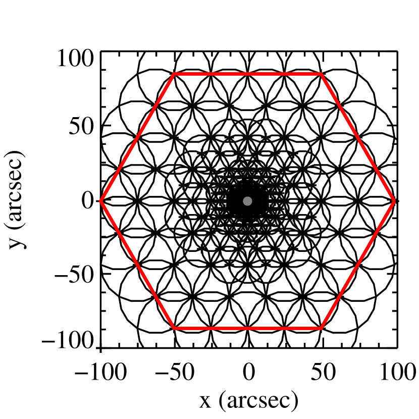
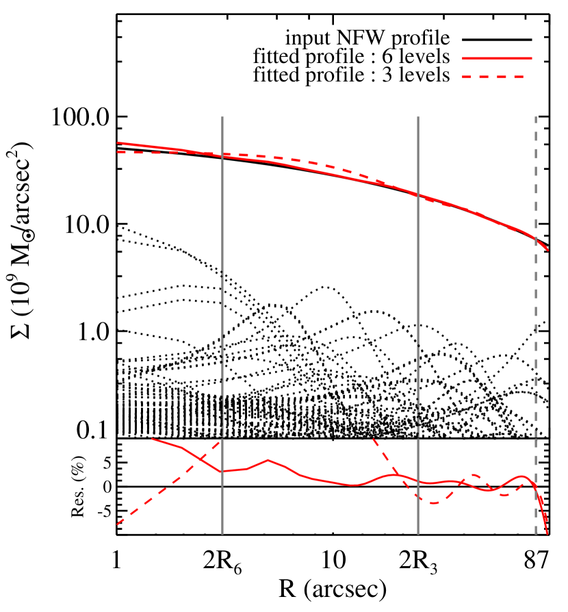
With enough resolution multi-scale models can reproduce all sorts of input mass distributions, provided of course that no region has a slope steeper than $\Sigma\propto r^{-3}$ (steepest slope of the TIMD potential). As an exercise, let us consider the input mass map produced by a cluster at a redshift $z=0.184$ whose density profile follows a circular NFW profile with a concentration of 5 and a scale radius of 150”. We compute a 200 x 200 arcsec² pixelated mass map of this object (i.e. about an ACS field of view) to be used as input mass map. To build the multi-scale grid, we start with an hexagon whose centre matches the centre of the NFW mass distribution and whose radius is set to 100”. We set the splitting threshold to $4.7\ 10^{10}M\odot/arcsec^{2}$, and limit to $n=6$ the number of recursive splitting. Fig. 2 shows the produced multi-scale grid. The smallest triangle, i.e. the smallest element of resolution, is $R_{6}=\frac{100^{\prime\prime}}{2^{6}}=1.54^{\prime\prime}$ wide. The grid contains 229 nodes, to which we associate RBF with TIMD profile. Their weight $\sigma_{i}^{2}$ are obtained by inverting Eq. 9. Note however, that we prefer an iterative method rather than a direct matrix inversion. Indeed, if we directly invert matrix $M$, we obtain a perfect fit but the solution vector contains negative $\sigma^{2}_{i}$, i.e. RBF with negative density profiles. Although Liesenborgs et al. (2008) allow some RBF to be negative, we are more conservative and prevent any element from the $\sigma_{i}^{2}$ vector from becoming negative. To do so, we minimise the following quantity

$$Z=\sum_{j=1}^{N}\left(S_{\mathrm{input}}(\theta_{j})-S_{\mathrm{pred}}(\theta_{j})\right)^{2}\;,$$ (11)

where $S_{\mathrm{input}}$ and $S_{\mathrm{pred}}$ are the input and predicted $S_{i}$ quantities of Eq. 9. With this iterative inversion technique, we can force the RBF to have positive weights $\sigma_{i}^{2}$, hence make sure that the overall surface density is positive. This way, we also avoid an additional regularisation term (and possible related effects on the final results) to control the sign of the surface density in the lensing $\chi^{2}$ defined below in Eq. 12.

Fig. 3 shows the reconstructed radial density profile. Note how well the arrangement of RBF fits the input NFW density profile. The residual is lower than 5% on the meaningful domain from twice $R_{6}$ to the hexagon inner limit. Note that a similar residual is also achieved with 3 levels of splitting, though on the corresponding meaningful domain. Therefore, a large number of splitting is not expressly justified unless the very centre of the mass distribution is of particular interest regarding some strong lensing constraints (e.g. radial arcs).

4 Multi-scale model of Abell 1689

Figure 4: Multi-scale grid made of 120 RBF obtained with 3 levels of splitting, and based on the input mass map of Abell 1689 (Limousin et al., 2007).

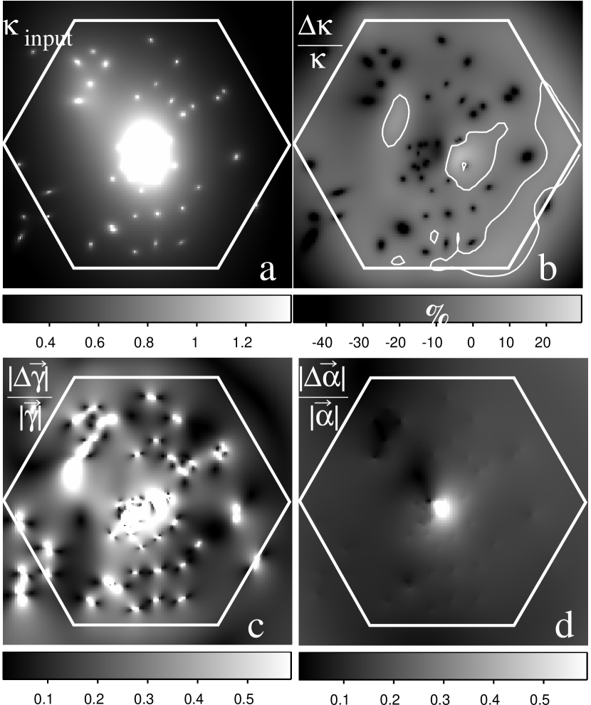
In this section, we continue to study the capabilities of multi-scale models. However, in place of an NFW mass distribution, we build the grid from a more realistic input mass map based on a simplified version of the mass model of the galaxy cluster Abell 1689 reported in Limousin et al. (2007). In fact, our input model is made of 2 cluster-scale and 60 galaxy-scale clumps of mass, instead of the 190 galaxy-scale clumps used in Limousin et al. Only massive clumps producing a deflection angle larger than 0.07” (i.e. roughly the HST/ACS imaging resolution) have been retained. All these clumps are described by PIEMD potentials. The galaxy-scale clumps are associated to cluster member galaxies. They follow scaling relations with similar properties as the one reported in Limousin et al. Fig. 5a shows the convergence map produced by this model ( with $\Sigma_{crit}=2\,10^{10}\,M_{\odot}/\mathrm{arcsec}^{2}$ calculated for a lens at redshift $z_{l}=0.184$ and a source at redshift infinity).

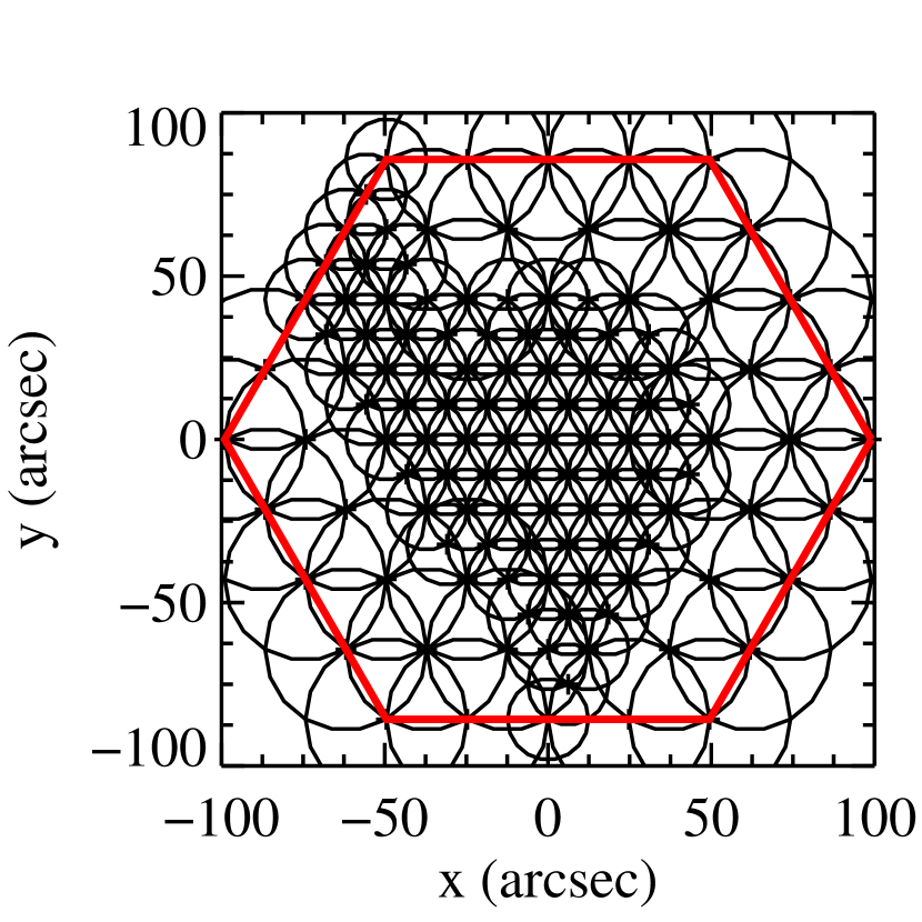
Following the same scenario as in the previous section, we start building the multi-scale grid by bounding the field of interest with an hexagon of radius 100” centered on the image centre, also the cluster centre. We set the splitting threshold to the critical surface density stated above. Doing so, we only oversample the central and North-East strong lensing regions, within which $\kappa>1$. Since the particular distribution and shape of the observed multiple images depend on the mass distribution in these regions, it is important to give them as much flexibility as possible. In a first attempt, we stop the levels of recursive splitting at 3. We obtain a grid of 120 RBF shown in Fig. 4. The size of the smallest triangle hence our smallest element of resolution is $R_{3}=12.3^{\prime\prime}$. In comparison, Limousin et al. (2007) estimate the core radius of the cluster to 33” which is more than twice $R_{3}$. According to the Shannon rule, we have therefore enough resolution to model it and reproduce central systems of multiple images. The weights $\sigma_{i}^{2}$ of the RBF are computed by iterative inversion of Eq. 9 as detailed previously.

Fig. 5 shows a disagreement between the convergence map produced by this model and the input one, above all at the galaxy-scale clumps location. Consequently, the multi-scale model underestimates by 9% the mass inside the hexagon. Beyond the hexagon limit, note the increasing disagreement between the 2 models. This is a modelling artefact of the multi-scale model due to the difference in slope between the RBF, which falls as $\Sigma\propto r^{-3}$, and the input profile slope, which falls as $\Sigma\propto r^{-1}$. Of course, such inaccuracies in the convergence map induce serious discrepancies in terms of shear and deflection angle. Fig. 5c shows large errors in the shear map at the galaxy-scale clumps location, but smaller errors far from these regions. In contrast, Fig. 5d shows that in the deflection angle map, discrepancies are weaker, with only 10% of disagreement throughout. Note that the discrepancy observed at the very centre is due to the lack of resolution of the multi-scale model. Therefore, we conclude that the lack of resolution of the multi-scale model at the galaxy-scale clumps location severely affects the lensing properties of the model.

Of course, more levels of splitting could improve the recovery, as demonstrated in the previous section with the NFW profile. However here, with 4 levels of splitting, the number of RBF raises to 318, and with 6 levels, it amounts to 4287. Optimising grids with so many clumps is currently beyond our computational resources.

Figure 5: (a) Input convergence map of the galaxy cluster Abell 1689 for a source at redshift $z_{s}=3$. The hexagon of radius 100”, bounds the region covered by the multi-scale grid. (b) Relative error map $(\kappa_{grid}-\kappa_{input})/\kappa_{input}$ in percent. The white contours correspond to $\Delta\kappa=0$. On average, the multi-scale model underestimates the surface density. (c) Relative shear error map $|\vec{\gamma}_{grid}-\vec{\gamma}_{input}|/|\vec{\gamma}_{input}|$. (d) Relative defection angle error map $|\vec{\alpha}_{grid}-\vec{\alpha}_{input}|/|\vec{\alpha}_{input}|$.

4.1 Adding galaxy halos

Instead of blindly increasing the level of splitting, we better build a multi-scale model including both a multi-scale grid and galaxy-scale clumps. The grid thus becomes a flexible mass component to fit the cluster-scale distribution of mass, whereas galaxy-scale clumps fit small-scale irregularities. This appears as a cheap solution to our problem of resolution.

5 Strong lensing constraints on multi-scale model

5.1 Methodology

In this section, we investigate the ability at constraining such multi-scale models with strong lensing and compare the results in terms of mass distribution and image prediction RMS, to a reference analytical model. This comparison is performed on the observational data of the galaxy cluster Abell 1689. First, we describe the Bayesian MCMC sampler we use to optimise the parameters. Second, we present the multi-scale and the reference models, their free parameters, assumed priors, and the strong lensing constraints. Finally, we analyse the results.

5.2 Bayesian MCMC sampler

Given their large number free parameters and the few number of constraints provided by strong-lensing data, “non-parametric” models are usually under-constrained, hence the regularisation terms to obtain smooth mass distribution (Marshall et al., 2002; Bradač et al., 2005; Suyu et al., 2006). In contrast, we do not use explicit regularisation term because our arrangement of RBF into a regular grid, and the smooth and everywhere positive TIMD profile describing them, constitute an intrinsic regularisation scheme. In addition, equating the TIMD core radius of the RBF to the grid resolution impedes strong discontinuities in the produced mass maps. Finally, the overlap of nearby RBF correlates the model’s parameters and makes them dependent, thus reducing the effective number of free parameters. The number of constraints may then become larger than the number of effective parameters, and multi-scale models may not be under-constrained (see Section 6).

In order to check our Bayesian MCMC sampler (based on the BayeSys library (Skilling, 2004) implemented in lenstool (Kneib et al., 1993; Jullo et al., 2007)), we generate a mock catalogue of 12 sources and 35 multiple images with the multi-scale model described above. Then, we check that the mass distribution estimated from this catalogue matches the input one. The $\chi^{2}$ is computed in the source plane for simplicity and computation time. For each system $i$ containing $n_{i}$ multiple images, we define $\chi^{2}_{i}$ as

$$\chi^{2}_{i}=\sum_{j=1}^{n_{i}}\left(\frac{\beta_{j}-\langle\beta\rangle}{\mu_{j}^{-1}\sigma_{j}}\right)^{2}\;,$$ (12)

where we use the lensing equation (Eq 1) to compute the source position $\beta_{j}$ of the observed image $j$, $\langle\beta\rangle$ is the barycentre of the $\beta_{j}$, $\mu_{j}$ is the magnification for image $j$, and $\sigma_{j}$ is the observational error at the position of image $j$.

Fortunately, we detect no systematics in the recovery. The error between the recovered and the input density maps is about 1% on average in the hexagon. The most outstanding result is that the algorithm converged towards the best fit region with only $3\times 10^{8}$ $\chi^{2}$ in less than 10 hours on a 2.4 Ghz processor, i.e. it performed more than 9000 $\chi^{2}/s$ on average and computed only 1.17 $\chi^{2}$ point per dimension. Note that a standard gradient method would have required at least 3 $\chi^{2}$ points per dimension to find a minimum i.e. $3^{122}=10^{58}$ $\chi^{2}$ points.

5.3 Multi-scale model and priors

Table 2: Priors the multi-scale model

Nb. clumps	$r_{cut}/r_{core}$	Level of splitting	$\sigma_{i}$	$r_{core}^{\star}$	$r_{cut}^{\star}$	$\sigma_{0}^{\star}$	$m_{K}^{\star}$
120+60	3	3	[0,1922] km/s	0.03”	[1,40]”	[10,400] km/s	16

We consider the multi-scale model of section 4 to which we add galaxy-scale clumps. The model then contains a multi-scale grid of 120 RBF, its smallest element of resolution is $R_{3}=12.3^{\prime\prime}$ and it has a ratio $r_{cut}/r_{core}=3$. We fix the profile and positions of the RBF. Their weights $\sigma_{i}^{2}$ are the only free parameters. We allow them to vary along a flat prior within the range 0.1 and 1.9 times the values found in section 4 by iterative inversion of Eq. 9. As indicative values, the minimum and maximum limits we assign are 0 km/s and 1922 km/s. This way, we prevent the model from wandering too far from the input mass map, but still give it a substantial freedom. We also add the 60 galaxy-scale clumps retained in section 4. We assume that (i) their position, ellipticity and orientation correspond to the brightness profile of their associated galaxy, (ii) their mass is proportional to the total luminosity of the galaxy, i.e. they all have the same M/L ratio and (iii) they are described by PIEMD potentials and their PIEMD parameters are linked by the following scaling relations

$$r_{core}=r_{core}^{\star}\left(\frac{L}{L^{\star}}\right)^{1/2}\;,r_{cut}=r_{cut}^{\star}\left(\frac{L}{L^{\star}}\right)^{1/2}\;,\sigma_{0}=\sigma_{0}^{\star}\left(\frac{L}{L^{\star}}\right)^{1/4}\;,$$ (13)

where $L^{\star}$, $r_{core}^{\star}$, $r_{cut}^{\star}$ and $\sigma_{0}^{\star}$ are respectively the luminosity and the three PIEMD parameters of a typical early-type galaxy at the cluster redshift. We consider a cluster galaxy with luminosity $L^{\star}$ corresponding to an F775W magnitude of 17.54. We know from previous studies in this cluster that $r_{cut}^{\star}\simeq 13^{\prime\prime}$ (Limousin et al., 2007; Halkola et al., 2007). Still, we assume a flat prior between 1” and 30” in order to investigate the possible interactions between the grid and galaxy-scale clumps. Accordingly, we assume $\sigma_{0}^{\star}$ vary along a wide flat prior defined on the range 10 and 400 km/s. Finally, recent studies have shown that the density profile of early-type galaxies in the field is singular up to observational limits (Koopmans et al., 2006; Czoske et al., 2008). Therefore, we fix $r_{core}^{\star}$ to 0.03” (i.e. a small value but different from zero for numerical reasons). In total, this multi-scale model sums 122 free parameters, whose priors are reported in Table 2.

Finally, note that all the parameters used to build the multi-scale grid (e.g the input mass map, the hexagonal shape, the hexagon size, the splitting algorithm, the level of splitting, the $r_{cut}/r_{core}$ ratio and the surface density threshold) can potentially affect the inferred strong lensing mass distribution, and as such must be considered as priors as well. We further discuss this point in section 6. In particular, we look how the RMS of predicted multiple images improves with the number of splitting levels.

5.4 Reference model

As a reference model, we use a modified version of the Limousin et al. model with 2 cluster-scale clumps (for the main and the North-East halos), 3 galaxy-scale clumps described by individual PIEMD potentials to model the brightest cluster galaxy (BCG) and Galaxy 1 and Galaxy 2 that strongly affect systems 6, 24 and systems 1, 2 respectively, and the 60 galaxy-scale clumps of the multi-scale model described by scaling relations. In total, the reference model sums 33 free parameters, whose priors are reported in Table 3.

Table 3: Priors on the reference model

ID	R.A.	Decl.	$e$	$\theta$	$r_{core}$(kpc)	$r_{cut}$(kpc)	$\sigma_{0}$(km/s)
Clump 1	[-15,15]	[-15,15]	[0.1,0.55]	[0,180]	[30,150]	1500	[1000,1700]
Clump 2	[-90,-35]	[5,79]	[0.4,0.9]	[0,180]	[25,90]	500	[300,650]
BCG	[-10,10]	[-10,10]	[0,0.6]	[0,180]	[0.1,10]	[9,550]	[300,680]
Galaxy 1	49.0	31.5	[0,0.9]	[0,180]	[0.1,30]	[9,180]	[150,280]
Galaxy 2	[-49,-45]	[27,35]	[0,0.9]	[0,180]	[0.1,20]	[4,190]	[200,580]
$L^{\star}$ elliptical galaxy	…	…	…	…	0.15	[20,60]	[150,280]
Notes : Coordinates are given in arcseconds with respect to the BCG (R.A. = 13:11:29 Decl. = -01:20:27).
The ellipticity $e$ is the one of the mass distribution, expressed as $a^{2}-b^{2}/a^{2}+b^{2}$.

5.5 Strong lensing constraints in Abell 1689

Table 4: Multiply imaged systems used as constraints

ID	R.A.	Decl.	$\langle\chi^{2}\rangle$	$z_{spec}$	Image plane rms (arcsec) Multi-scale model	Image plane rms (arcsec) Reference model
1……………			1.91	3.0	0.71	0.67
1.1………….	13:11:26.44	-1:19:56.37	0.96		0.99	0.94
1.3………….	13:11:29.76	-1:21:07.31	0.96		0.09	0.16
2……………			1.28	2.5	0.28	0.59
2.1………….	13:11:26.52	-1:19:55.07	0.64		0.40	0.78
2.4………….	13:11:29.80	-1:21:05.95	0.64		0.08	0.29
4.1………….			5.07	1.1	0.22	0.67
4.11…………	13:11:32.16	-1:20:57.33	1.23		0.27	0.85
4.12…………	13:11:30.51	-1:21:11.90	0.90		0.25	0.89
4.13…………	13:11:30.75	-1:20:08.01	1.64		0.14	0.19
4.14…………	13:11:26.28	-1:20:35.06	1.30		0.21	0.50
4.2………….			1.33	1.1	0.18	1.08
4.21…………	13:11:32.10	-1:20:58.31	0.66		0.17	1.29
4.22…………	13:11:30.65	-1:21:11.41	0.66		0.18	0.83
5……………			4.35	2.6	0.36	1.01
5.1………….	13:11:29.06	-1:20:48.41	2.18		0.49	2.18
5.3………….	13:11:34.11	-1:20:20.87	2.18		0.15	0.49
6……………			1.73	1.1	0.17	0.31
6.1………….	13:11:30.75	-1:19:37.90	0.87		0.21	0.40
6.2………….	13:11:33.34	-1:20:11.97	0.87		0.11	0.16
7……………			1.93	4.8	0.16	0.23
7.1………….	13:11:25.44	-1:20:51.52	0.96		0.19	0.23
7.2………….	13:11:30.67	-1:20:13.79	0.96		0.12	0.23
10.1…………			0.84	1.8	0.10	0.27
10.11………..	13:11:33.96	-1:20:50.99	0.42		0.09	0.28
10.12………..	13:11:28.05	-1:20:12.28	0.42		0.10	0.26
10.2…………			0.68	1.8	0.08	0.18
10.21………..	13:11:33.95	-1:20:51.54	0.34		0.08	0.20
10.22………..	13:11:28.08	-1:20:11.84	0.34		0.08	0.17
10.3…………			0.77	1.8	0.08	0.19
10.31………..	13:11:33.96	-1:20:51.53	0.39		0.08	0.20
10.32………..	13:11:28.08	-1:20:12.24	0.39		0.09	0.18
24.1…………			3.34	2.6	0.17	0.52
24.11………..	13:11:29.18	-1:20:56.04	1.63		0.18	0.79
24.13………..	13:11:30.29	-1:19:33.86	0.78		0.20	0.25
24.14………..	13:11:33.71	-1:20:19.82	0.94		0.13	0.33
24.2………..			2.92	2.6	0.18	0.40
24.21………..	13:11:29.22	-1:20:55.28	0.77		0.15	0.38
24.23………..	13:11:30.25	-1:19:33.26	1.30		0.25	0.55
24.24………..	13:11:33.69	-1:20:18.80	0.85		0.12	0.21

From Limousin et al. (2007) we select a catalogue of 28 images in 12 systems of multiple images (see Table 4). We will use the rest of the images later to check for model predictability and over-fitting. Selected images must have a measured spectroscopic redshift (Richard et al., prep.), or present at least two star-forming regions clearly visible in all the counter-images, in order to avoid identification mistakes. We also remove images whose light is blended with the light of nearby galaxies. To get accurate measurements of the images positions, we fit a Gaussian profile to their light distribution with the IRAF task imexam. Because our selection mostly contains compact images, we measure a Gaussian width of 0.13” on the position measurements. We use this positional error for all the images in the lensing $\chi^{2}$ (Eq.12). Since we only use the image position as a constraint, we sum 32 constraints.

5.6 Computational considerations

On a 2.4 Ghz processor, the Bayesian estimation of the 122 free parameters took 15 days to produce about 20000 MCMC samples. Although it could be considered as quite computational intensive, considering the number of free parameters and the fact that we not only find the best fit region but also explore the parameter space in its neighbourhood, it is in fact very efficient. In the last section, we discuss some issues related to the number of samples.

5.7 Results

5.7.1 Images prediction

Results confirm the ability of multi-scale models at being used as lens models. Indeed, the RMS per system and per image reported in Table 4 and shown in Fig. 7a highlight the good precision we obtain. The RMS averaged over all the systems is 0.28”. In contrast, the reference model optimised with the same catalogue of images produces a mean RMS of 0.54”. For all the systems unless System 1, RMS with the multi-scale model are lower than RMS with the reference model. System 1 has a slightly larger RMS because the galaxy-scale clump located 3.2” to the West may not fit the same scaling relations as the other galaxy-scale clumps. Indeed, if we assume that 2 galaxies do not follow the same scaling relations, there is no perfect solution for the scaling relations parameters. The images producing the largest $\chi^{2}$ bias the scaling relations in their favor. The fit of images with a lower $\chi^{2}$ but close to galaxies following other scaling relations worsens. In this respect, note that for System 1, $\chi^{2}=1.91$ and RMS$=0.71^{\prime\prime}$ whereas for System 24.1 $\chi^{2}=3.34$ and RMS$=0.17^{\prime\prime}$. Both systems are at the same distance of a galaxy-scale clump. System 24.1 is therefore likely biasing the scaling relations in its favor.

Figure 6: Relative contributions of the PCA eigenvalues to the total variance of the samples distribution in the our parameter space with 122 dimensions. Note that 90% of the variance is reproduced with only 12 effective parameters.

Given the large number of free parameters compared to the number of constraints, we could have expected better RMS and smaller $\chi^{2}$. Indeed, it is usually accepted that models with more free parameters than constraints allow an infinity of perfect solutions. Since our solutions are not perfect, it means that the number of useful effective parameters in our model is actually lower than the number of constraints. To estimate this number, we analyse the distribution of the MCMC samples in the parameter space by means of the Principal Component Analysis (PCA) technique. Fig. 6 shows that 90% of the variance of the distribution is reproduced with only 12 effective parameters out of the 122 ‘real’ parameters. With the reference model, 90% of the variance is reproduced with only 10 effective parameters out of the 33 ‘real’ ones. In both cases, the number of effective parameters is lower than the 32 constraints, hence the non perfect fit. Though very interesting, investigating the physical meaning of these effective parameters is out of the scope of this paper.

Figure 7: (a) Image plane RMS of the images used as constraints in function of their distance to the closest galaxy. In black: RMS obtained with the multi-scale model. In red: RMS with the reference model. (b) RMS produced by the images kept for the over-fitting check. The two subsets give similar RMS, indicating no particular sign of over-fitting with the multi-scale model.

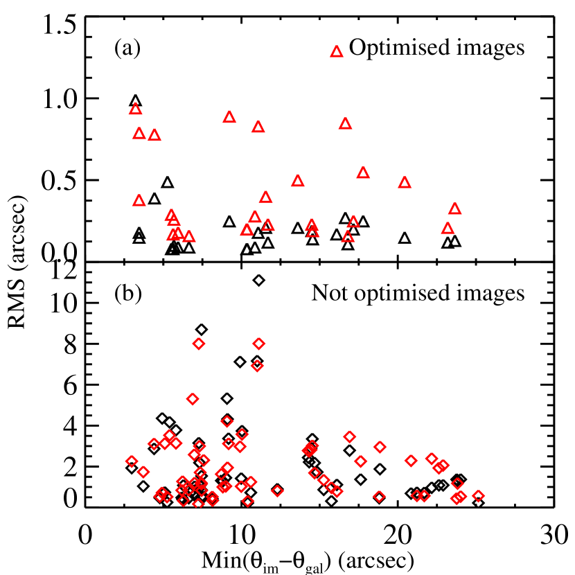
As a definite confirmation that our multi-scale model is not under-constrained and do not over-fit the data, we apply the cross-checking technique : with both the multi-scale and the reference models, we predict the images positions for the part of the images catalogue not used as constraints, and compare the RMS between predicted and observed positions. This way, if a model is biased towards the subset of images used as constraints, it should be unable to give accurate predictions. Fig.7b shows the RMS given the two models for the not optimised part of the images catalogue. On average, we find an RMS of 3.32” for the multi-scale model and an RMS of 3.49” for the reference model. Since the two models give similar predictions, we conclude that the multi-scale model does not over-fit the data.

In addition, Fig. 7b also shows that when images get closer to galaxies their RMS increases. This increasing RMS again suggests that galaxy-scale clumps do not perfectly fit the imposed scaling relations. There must exists a scatter in the scaling relations that images seem to be sensible to, and that should be included in our future models.

5.7.2 Convergence, deviation and shear maps

Figure 8: Comparison between maps obtained with the reference model (left column) and the multi-scale model (middle column). The color images correspond to the relative difference $|\mathrm{Reference}-\mathrm{grid}|/|\mathrm{Reference}|$ between the two maps in grey. All the maps are computed for a source plane at redshift $z_{S}=3$. The red hexagon marks the limit of the multi-scale grid beyond which the maps become meaningless. The black crosses in the color images mark the positions of the images used as constraints.

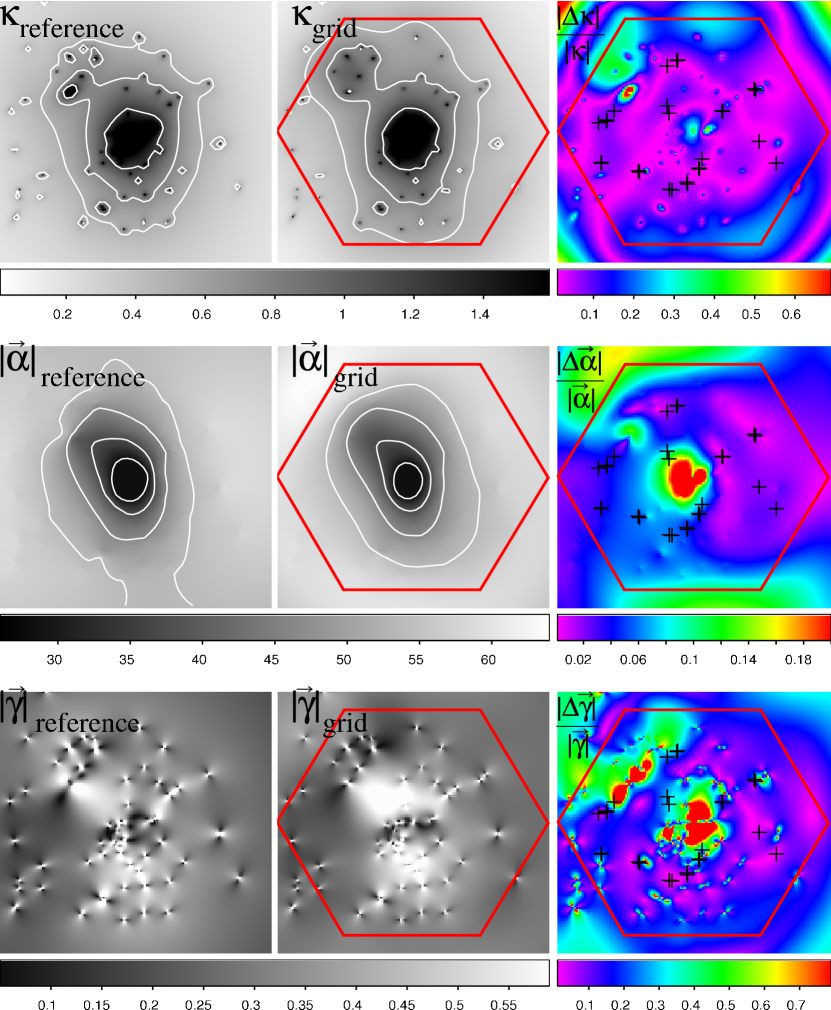
Fig. 8 compares mean convergence, deviation and shear maps produced with the reference and the multi-scale models. To produce these maps, we compute the convergence, deviation and shear maps for each mass model of the MCMC chain, and compute the mean maps by averaging the values of each pixel of each map. First of all, note that the two convergence maps are very similar. The better RMS obtained with the multi-scale model does not originate from any particular missing clump in the reference model. The mass enclosed at the Einstein radius $M(<45^{\prime\prime})$ are also very similar with less than 1% difference. In other words, the “mass follows light” assumption in traditional modelling holds. Nonetheless, the better RMS obtained with the multi-scale model attests a significantly higher degree of flexibility. In particular, we note that in the convergence map, the North-East clump, at intermediate scale between cluster and galaxy scale, looks smoother and more detached from the main clump than in the convergence map produced by the reference model. The deviation maps produced by the two models are also very similar with less than 5% of difference at the images position. Finally the errors in the shear maps are mostly lower than 10% at the images position. This is currently below what we can observationally constrain by measuring the ellipticity of multiple images. Consequently, the better RMS with the multi-scale model is merely due to its large number of free parameters, which allow a refined modelling of the mass distribution irregularities at intermediate scale between cluster and galaxy scale.

5.7.3 Error mass map

Figure 9: Map of S/N ratio. Coloured contours bound regions with S/N greater than 300, 200, 100 and 10, the highest S/N region being at the centre. Red contours are mean iso-mass contours from 5 to $0.77\times 10^{12}\ M_{\odot}/\mathrm{arcsec}^{2}$ by steps of 1 and $0.5\times 10^{12}\ M_{\odot}/\mathrm{arcsec}^{2}$ for the three outer contours. This map has been computed with 20000 MCMC samples. Black boxes mark the positions of the multiple images used to constrain the mass distribution.

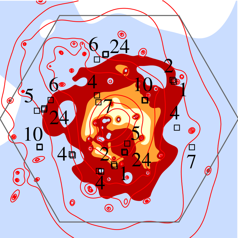
In addition to the mean convergence map, the Bayesian approach also allows to compute the standard deviation and the $S/N$ convergence maps. Fig. 9 shows that the mass distribution is estimated with high confidence, since the $S/N$ is everywhere larger than 10 inside the hexagon, i.e. less than 10% error. This means that the correlations between the RBF parameters, highlighted by the PCA technique, must strongly restrict the range allowed by the priors, hence the small error. Furthermore, the smooth iso-mass contours confirm the ability of multi-scale models at producing smooth mass maps.

6 Discussion

In the previous section, we have worked at demonstrating the strength of our model. We are now going to highlight some critical aspects which will give the reader a more complete view of the multi-scale models, but also of “non-parametric” models in general, for which the effects of grid parameters on the final results are rarely investigated in details. In this section, we particularly investigate two parameters : (i) the $r_{cut}/r_{core}$ ratio defining the RBF concentration and (ii) the level of splitting. We do not investigate the threshold parameter because we only aim at oversampling strong lensing regions. Therefore hereafter, in all the models, the surface density threshold is set equal to $\Sigma_{crit}=2\times 10^{10}\;M_{\odot}/\mathrm{arcsec}^{2}$.

To begin with, we build 5 multi-scale models similar to the one used so far, but with different $r_{cut}/r_{core}$ ratios and levels of splitting. Some models built with 3 levels of splitting have 127 clumps because the grid has been shifted by 6” with respect to the input mass map. We found that this shift does not affect the final results. We optimise each model with our catalogue of 28 images and report the mean RMS and mean likelihood $\langle\log(L)\rangle=-0.5\;\langle\chi^{2}\rangle$ in Table 5. Note also that less MCMC samples have been gathered with models A and C in order to evaluate how the number of MCMC samples affects the error estimation.

Table 5: List of multi-scale models used in this section

ID	$r_{cut}/r_{core}$ ratio	Nb of splitting levels	Nb of clumps	Nb samples	$M_{gal}/M_{tot}$ ratio	Mean Image plane rms	$\langle\log(L)\rangle$
A	2	3	127	439	14%	0.23”	-14.8
B	3	3	120	20920	13%	0.27”	-13.4
C	4	3	127	369	12%	0.33”	-28.2
D	10	3	127	25029	11%	0.86”	-228.2
E	3	4	318	38399	5%	0.22”	-13.1
Reference	-	-	-	1000	22%	0.57”	-59.4

6.1 The $r_{cut}/r_{core}$ ratio

Figure 10: Confidence intervals at 68% and 99% of the scaling relations parameters $r_{cut}^{\star}$ and $\sigma^{\star}$ obtained with models A, C and D. Dashed lines show the curves of constant M/L ratio within a 60” aperture (i.e. the mean distance from multiple images to galaxy-scale clumps). In black is shown the same curve but for the Limousin et al. model. The vertical dashed limit at $2R_{3}=24.6^{\prime\prime}$ marks the grid resolution of model A. The grid resolution of models C and D at $4R_{3}$ and $10R_{3}$ respectively, are beyond the abscissa scale limit of this plot. This figure shows that galaxy-scale clumps efficiently increase the grid resolution.

Figure 11: Histograms of the RBF velocity dispersions in models A, B, C and D, as distributed before strong lensing optimisation (these distributions slightly shrink after optimisation, i.e. small values get larger and large values get smaller). Note that multi-scale models are mainly made of RBF with small velocity dispersion. As RBF get more extended, more RBF are assigned small velocity dispersions.

The $r_{cut}/r_{core}$ ratio characterises the concentration of the RBF. Models with small ratios are more flexible because their RBF are more independent. Table 5 shows that such models better fit multiple images but can also over-fit them. In contrast, models with larger ratios produce more extended and overlapping RBF, which worsens the fit to multiple images. For instance, model A with $r_{cut}/r_{core}=2$ (i.e. with very concentrated RBF) gives a better fit than model D, with $r_{cut}/r_{core}=10$. If we calculate their likelihood ratio we find $\log(L_{D}/L_{A})=113$, which means that model D is clearly ruled out.

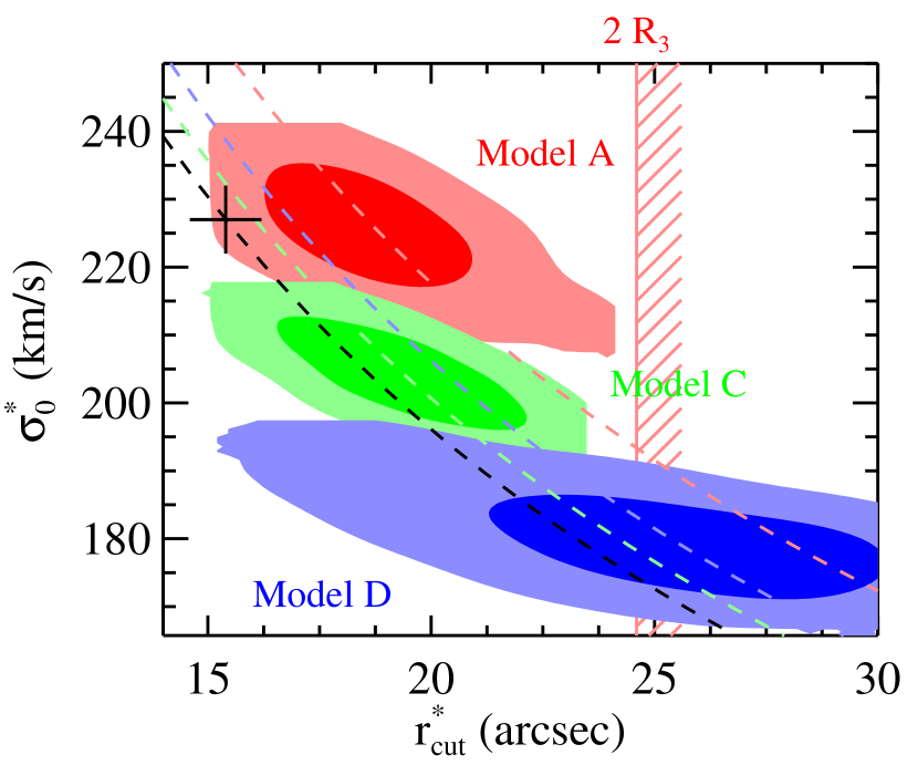
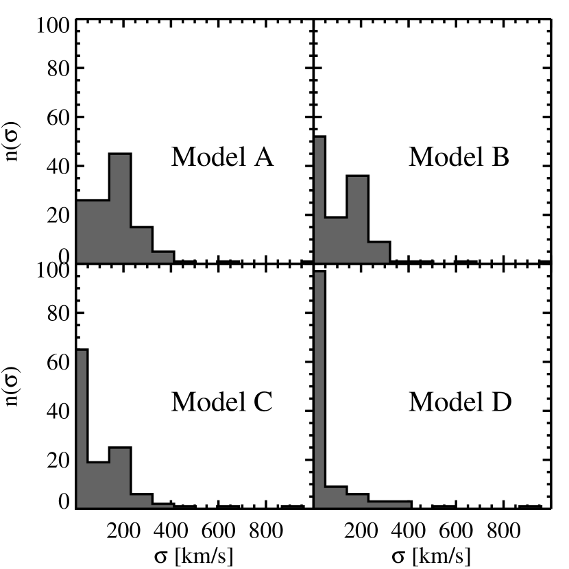
In addition to the fit quality, the $r_{cut}/r_{core}$ ratio affects the scaling relations parameters $r_{cut}^{\star}$ and $\sigma_{0}^{\star}$. Fig. 10 shows that models with large $r_{cut}/r_{core}$ ratio (i.e. extended RBF) induce large $r_{cut}^{\star}$ and small $\sigma_{0}^{\star}$. To understand this behaviour, Fig. 11 shows that in such models, most of the RBF have a small velocity dispersion, i.e. little weight. The mass distribution must then be very smooth with only a few very extended and effective RBF. The $r_{cut}^{\star}$ extension parameter becomes large, in order for the galaxy-scale clumps to accommodate the multiple images and compensate for the lack of effective RBF in their neighbourhood. Besides, whatever the $r_{cut}/r_{core}$ ratio, Fig. 10 shows that the curves of constant M/L ratio agree at 2$\sigma$, and Table 5 shows that for a given level of splitting, the $M_{gal}/M_{tot}$ ratios are similar. In conclusion, the $r_{cut}/r_{core}$ ratio affects the extension of the galaxy-scale clumps but do not affect their mass.

Figure 12: Convergence profiles obtained with models A, C and D. Larger $r_{cut}/r_{core}$ ratios make the profile shallower. The vertical arrows radially locate the strong lensing constraints.

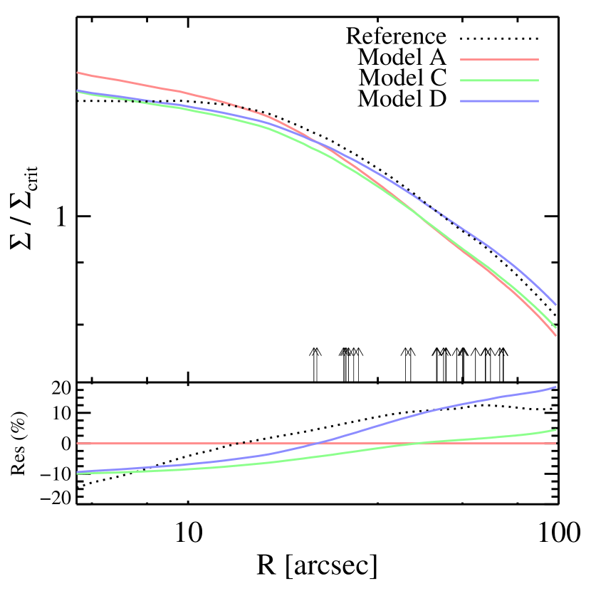
As already noticed by Diego et al. (2007), extended RBF produce a mass sheet excess at large radius. Fig. 12 shows that model D with a large $r_{cut}/r_{core}$ ratio produces a density profile with a shallower slope than model A. Since with larger ratios, the RBF become more extended, their cut-off radius is pushed out to larger radius. Their isothermal slope is maintained over a wider range in radius, making the total density profile shallower.

6.2 The level of splitting

Figure 13: Density profile comparison between multi-scale models obtained with 3 and 4 levels of splitting, hence made of 120 and 318 RBF respectively, and 60 galaxy-scale clumps. The vertical arrows radially locate the strong lensing constraints. In this region, the density profiles are similar. Outside, their are mostly driven by the priors.

Figure 14: Confidence levels at 68% and 99% of the scaling parameters $r_{cut}^{\star}$ and $\sigma_{0}^{\star}$ recovered with multi-scale models B (green) and D (blue). Dashed lines show the curves of constant M/L ratio within a 60” aperture. Dashed limits at $3R_{3}$ and $3R_{4}$ mark the extension of the smallest RBF for models B and D respectively. Note that with 4 levels, the galaxy-scale clumps are completely unconstrained because they directly compete with the RBF.

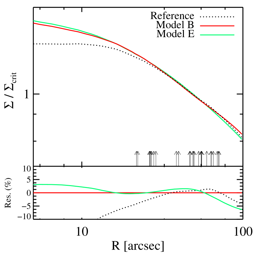
Another prior involved in the building of the grid is the level of splitting. Fig. 13 shows that in contrast to the $r_{cut}/r_{core}$ ratio, the level of splitting does not affect the slope of the density profile. The profiles obtained with models B, E and the reference model are very similar. In addition, Table 5 shows that models B and E have similar RMS and likelihood. Therefore, more levels of splitting is not expressly justified given the data. Note also that the reference model produces a similar density profile but has an RMS twice the RMS obtained with models B or E. Similar density profiles does not necessarily mean similar fit to the data.

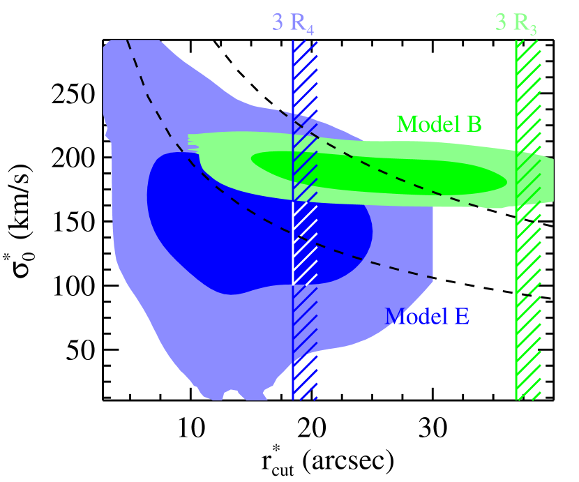
Fig. 14 shows that the level of splitting affects the scaling relations parameter $r_{cut}^{\star}$. With model E, $r_{cut}^{\star}\simeq 15^{\prime\prime}$ whereas with model B, $r_{cut}^{\star}\simeq 25^{\prime\prime}$. In addition, it shows that with model E, $r_{cut}^{\star}$ is close to the grid resolution $3R_{4}=18.4^{\prime\prime}$, whereas with model B, it is significantly smaller, since $3R_{3}=36.9^{\prime\prime}$. It seems therefore that by increasing the level of splitting, we just replace the galaxy-scale clumps by the RBF of the grid. The large errors in model E indeed indicate that the galaxy-scale clumps are not constrained anymore by the data. Besides, Fig. 14 and Table 5 show that the M/L ratio decreases as the level of splitting increases. The contribution of the galaxy-scale clumps to the total mass decreases from 13% in model B to 5% in model D. In other words, with 4 levels of splitting, galaxy-scale clumps do not help anymore in increasing the model resolution. The scaling relations inflexibility might imped them from decreasing in size, to make the model gain in resolution and improve the fit. Again, one solution could be to introduce a scatter in the scaling relations. We will explore this solution in a forthcoming paper.

6.3 Invariant quantity

Figure 15: Galaxy-scale clumps mass measurements within a 4” aperture, performed on pixelated mass maps resulting from the fit of models A, B, C, D and E to the same subset of multiple images. Measurements are very consistent with a scatter of about 10%, in agreement with the errors observed on the radial density profiles.

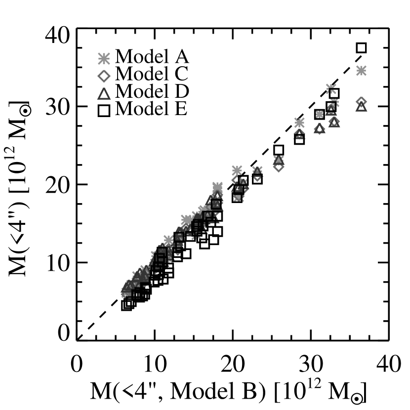
So far, we have found that both the $r_{cut}/r_{core}$ ratio and the level of splitting affect the estimation of the scaling relations parameters $r_{cut}^{\star}$, $\sigma_{0}^{\star}$, as well as the M/L ratio of the galaxy-scale clumps. In this context, studying the galaxy-scale clumps physical properties seems a little risky. Nevertheless, it is possible to get more reliable values by making measurements directly on the surface density maps. In Fig. 15, we compute the aperture mass of galaxy-scale clumps with Sextractor (Bertin & Arnouts, 1996) and pixelated mass maps obtained for models A, B, C, D and E. We choose Sextrator because it affords a multi-threshold algorithm to assign the mass in a pixel to the most credible of two nearby galaxies. We find that the masses enclosed in a 4” aperture (i.e. the smallest distance between two nearby galaxy-scale clumps) are almost unaffected by the grid parameters. The scatter is of the order of 10%, in agreement with the errors found in the density profiles. Estimating the galaxy-scale clumps properties directly from the surface density maps seems therefore a more reliable and better constrained solution (given the priors) than simply considering the $r_{cut}^{\star}$ and $\sigma_{0}^{\star}$ modelling parameters.

6.4 Errors analysis

As already stressed, given the size of the parameter spaces, it is encouraging to see our Bayesian MCMC sampler converging to the best fit region in less than 5000 samples. However, Fig. 14 shows that the error bars increase between model B and D. Since model D sums twice as many samples as model B, it seems that the estimation of the errors depends on the number of computed samples. To study the evolution of the errors estimation with the number of MCMC sample with the number of MCMC sampless, we define the cumulated relative error quantity computed over all the free parameters of the model as

$$\mathrm{Cumulated\ parameters\ error}=\sqrt{\sum_{i}\left(\frac{\sigma[X_{i}]}{E[X_{i}]}\right)^{2}}$$ (14)

where $\sigma[X_{i}]$ and $E[X_{i}]$ are the standard deviation and the mean value of the $X_{i}$ MCMC random variable for parameter $i$. Fig. 16 shows that this error has not converged even after more than 20000 samples. Similarly, we define the error on the density profile as

$$\mathrm{Density\ profile\ error}=\sqrt{\int_{0}^{100}\left(\frac{\sigma[S_{i}]}{E[S_{i}]}\right)^{2}\mathrm{d}R}$$ (15)

where $S_{i}$ is a random variable for the radial density profile integrated on the range 0 to 100”. In contrast to the error on the free parameters, Fig. 17 shows that the error on the density profile converges after only 1500 samples. Therefore, accurate errors on the mass distribution are fast to compute, whereas errors on the parameters of the model, such as $r_{cut}^{\star}$ or $\sigma_{0}^{\star}$ for instance, are difficult to estimate accurately and might actually be underestimated.

Figure 16: Evolution of the cumulated relative error of the parameters of model B in function of the number of MCMC samples. The error does not stabilise even after more than 20000 samples.

Figure 17: Evolution of the relative error on the radial density profile of model B in function of the number of MCMC samples. The error stabilises soon after 1500 samples.

7 Conclusion

In this paper, we present a multi-scale model sufficiently flexible to reproduce the observed systems of multiple images with high accuracy, but also robust against over-fitting. The model combines a grid of radial basis functions (RBF), and galaxy-scale clumps hosting cluster member galaxies, described by PIEMD potentials and scaling relations.

We apply this model to the galaxy cluster Abell 1689. We constrain the model with a subset of multiple images extracted from the Limousin et al. (2007) catalogue. We obtain an RMS between observed and predicted positions of 0.28” in the image plane, i.e. about half the RMS obtained with a slightly modified version of the Limousin et al. model (the reference model). We confirm predictability of our multi-scale model by cross-checking the optimised model with the part of the images catalogue not used as constraints. We find similar RMS with the multi-scale and the reference models. This confirms that we do not overfit the data, despite the large number of free parameters. We propose a Principal Component Analysis (PCA) technique to estimate the effective number of free parameters. We find that our multi-scale model with 122 parameters contains only 12 effective parameters. Our multi-scale model produces smooth mass maps and radial density profiles.

Then, we compare the convergence, deviation and shear maps obtained both with the multi-scale and the reference models. We find no major difference between the two sets of maps. This means that the better RMS is due to minor changes allowed by the flexibility of the multi-scale model at intermediate scale between cluster and galaxy scale. We also note that the galaxy-scale clumps are better integrated to the North-East cluster-scale clump with the multi-scale grid than with the traditional reference model. The better modelling of this cluster-scale component, embedded in projection in the main cluster core, thus illustrates how multi-scale models can reproduce irregular mass distributions.

Finally, we study how changes on the grid parameters affect the density profile, the scaling relations parameters $\sigma_{0}^{\star}$, $r_{cut}^{\star}$, and the M/L ratio of the galaxy-scale clumps. We find that galaxy-scale clumps efficiently increase the resolution of the grid of RBF without modifying the density profile. Excessively raising the level of splitting in order to increase the grid resolution is thus not expressly justified. We also find that the scaling relations parameter $r_{cut}^{\star}$, related to the galaxy-scale clumps extension, decreases as the RBF get more concentrated. This degeneracy leads to several models producing the same radial density profile. Fortunately, the likelihood is also significantly affected, hence allowing an effective model selection. In spite of this degeneracy between the model’s parameters, we propose a reliable solution to measure the galaxy-scale clump mass into an aperture directly on the mass maps produced by the optimised models. Indeed, we note that the model’s parameters degenerate, but the resulting mass distributions are little affected by the priors on the grid.

This work raises the issue of accurately measuring substructure properties in galaxy clusters (Halkola et al., 2007; Natarajan et al., 2007; Smith & Taylor, 2008). The degeneracy between galaxy-scale and cluster-scale mass components can potentially lead to spurious conclusions. In traditional modelling of observationally quiet clusters, whatever the priors on the adopted profile for the cluster-scale component (e.g. PIEMD or NFW profile), the substructure properties are little affected, given the constraints. However, in unrelaxed perturbed clusters, pursuing this study with the same technique appears to be more risky. Our multi-scale model as described above offers an interesting solution.

In terms of computation time, this method is still slow. We could make it faster by restricting the number of gradients and Laplacians calculated per image to solely the most significant. However, this has to be treated with care since the sum of negligible gradients can become significant. Missing such gradients could lead to spurious results. Look for instance Deb et al. (2008) to understand how complex it is to accurately select the relevant clumps for gradient calculation.

Multi-scale models open interesting avenues for the modelling of galaxy clusters. Indeed, today standard parametric methods are facing their own limitations. New lensing results reveal irregular or merging clusters (e.g. Bradač et al., 2006; Jee et al., 2007; Mahdavi et al., 2007). Multi-scale models with RBF afford the robustness of parametric methods as well as the flexibility of non-parametric methods. Since we use analytical potentials, the extension of the method to weak lensing is straightforward. We are currently working at combining strong and weak lensing signal to extend the accuracy of our modelling to larger radius. In inner regions, the strong lensing constraints will need a dense network of RBF to be reproduced accurately whereas in the outskirts, a coarser sampling will perfectly fit with the lower density of weak lensing constraints (see Jullo et al. in prep). This method can also be extended to multiplane lensing, allowing thus tomographic analysis.

The authors thank Phil Marshall, Harald Ebeling, Marceau Limousin and Johan Richard, as well as the referee for enlightening and fruitful comments. JPK and EJ thank support from CNRS and SL2S grant 06-BLAN-0067 from the Agence National de la Recherche.

References

- Bertin & Arnouts (1996) Bertin E., Arnouts S., 1996, Astronomy & Astrophysics Supplement, 117, 393
- Blandford & Narayan (1986) Blandford R., Narayan R., 1986, ApJ, 310, 568
- Bradač et al. (2006) Bradač M., Clowe D., Gonzalez A. H., Marshall P., Forman W., Jones C., Markevitch M., Randall S., Schrabback T., Zaritsky D., 2006, ApJ, 652, 937
- Bradač et al. (2005) Bradač M., Schneider P., Lombardi M., Erben T., 2005, A&A, 437, 39
- Broadhurst et al. (2005) Broadhurst T., Benítez N., Coe D., et al 2005, ApJ, 621, 53
- Clowe et al. (2006) Clowe D., Bradač M., Gonzalez A. H., Markevitch M., Randall S. W., Jones C., Zaritsky D., 2006, ApJ, 648, L109
- Coe et al. (2008) Coe D., Fuselier E., Benítez N., Broadhurst T., Frye B., Ford H., 2008, ApJ, 681, 814
- Czoske et al. (2008) Czoske O., Barnabè M., Koopmans L. V. E., Treu T., Bolton A. S., 2008, MNRAS, 384, 987
- Czoske et al. (2002) Czoske O., Moore B., Kneib J.-P., Soucail G., 2002, A&A, 386, 31
- de Blok et al. (2003) de Blok W. J. G., Bosma A., McGaugh S., 2003, MNRAS, 340, 657
- Deb et al. (2008) Deb S., Goldberg D. M., Ramdass V. J., 2008, The Astrophysical Journal, 687, 39
- Diego et al. (2005) Diego J. M., Protopapas P., Sandvik H. B., Tegmark M., 2005, MNRAS, 360, 477
- Diego et al. (2007) Diego J. M., Tegmark M., Protopapas P., Sandvik H. B., 2007, MNRAS, 375, 958
- Elíasdóttir et al. (2009) Elíasdóttir Á., Limousin M., Richard J., Hjorth J., Kneib J.-P., Natarajan P., Pedersen K., Jullo E., Paraficz D., 2009, ArXiv e-prints
- Fu et al. (2008) Fu L., Semboloni E., Hoekstra H., Kilbinger M., van Waerbeke L., Tereno I., Mellier Y., Heymans C., Coupon J., Benabed K., Benjamin J., Bertin E., Doré O., Hudson M. J., Ilbert O., et al. 2008, A&A, 479, 9
- Gavazzi et al. (2007) Gavazzi R., Treu T., Rhodes J. D., Koopmans L. V. E., Bolton A. S., Burles S., Massey R. J., Moustakas L. A., 2007, ApJ, 667, 176
- Gentile et al. (2007) Gentile G., Tonini C., Salucci P., 2007, A&A, 467, 925
- Guzzo et al. (2008) Guzzo L., Pierleoni M., Meneux B., Branchini E., Le Fèvre O., Marinoni C., Garilli B., Blaizot J., De Lucia G., Pollo A., McCracken H. J., Bottini D., Le Brun V., Maccagni D., Picat J. P., Scaramella R., et al. 2008, Nature, 451, 541
- Halkola et al. (2006) Halkola A., Seitz S., Pannella M., 2006, MNRAS, pp 1133–+
- Halkola et al. (2007) Halkola A., Seitz S., Pannella M., 2007, ApJ, 656, 739
- Hu & Dodelson (2002) Hu W., Dodelson S., 2002, ARA&A, 40, 171
- Jee et al. (2007) Jee M. J., Ford H. C., Illingworth G. D., White R. L., Broadhurst T. J., Coe D. A., Meurer G. R., van der Wel A., Benítez N., Blakeslee J. P., Bouwens R. J., Bradley L. D., Demarco R., Homeier N. L., Martel A. R., Mei S., 2007, ApJ, 661, 728
- Jullo et al. (2007) Jullo E., Kneib J.-P., Limousin M., Elíasdóttir Á., Marshall P. J., Verdugo T., 2007, New Journal of Physics, 9, 447
- Kassiola & Kovner (1993) Kassiola A., Kovner I., 1993, ApJ, 417, 450
- Kneib et al. (1996) Kneib J.-P., Ellis R. S., Smail I., Couch W. J., Sharples R. M., 1996, ApJ, 471, 643
- Kneib et al. (1993) Kneib J. P., Mellier Y., Fort B., Mathez G., 1993, A&A, 273, 367
- Koopmans et al. (2006) Koopmans L. V. E., Treu T., Bolton A. S., Burles S., Moustakas L. A., 2006, ApJ, 649, 599
- Liesenborgs et al. (2007) Liesenborgs J., de Rijcke S., Dejonghe H., Bekaert P., 2007, MNRAS, 380, 1729
- Liesenborgs et al. (2008) Liesenborgs J., de Rijcke S., Dejonghe H., Bekaert P., 2008, MNRAS, 386, 307
- Limousin et al. (2005) Limousin M., Kneib J.-P., Natarajan P., 2005, MNRAS, 356, 309
- Limousin et al. (2007) Limousin M., Richard J., Jullo E., Kneib J. P., Fort B., Soucail G., Elíasdóttir A., Natarajan P., Ellis R. S., Smail I., Czoske O., Smith G. P., Hudelot P., Bardeau S., Ebeling H., Egami E., Knudsen K. K., 2007, ApJ, 668, 643
- Limousin et al. (2008) Limousin M., Richard J., Kneib J.-P., Brink H., Pelló R., Jullo E., Tu H., Sommer-Larsen J., Egami E., Michałowski M. J., Cabanac R., Stark D. P., 2008, A&A, 489, 23
- Mahdavi et al. (2007) Mahdavi A., Hoekstra H., Babul A., Balam D. D., Capak P. L., 2007, ApJ, 668, 806
- Marshall et al. (2002) Marshall P. J., Hobson M. P., Gull S. F., Bridle S. L., 2002, MNRAS, 335, 1037
- Massey et al. (2007) Massey R., Rhodes J., Ellis R., Scoville N., Leauthaud A., Finoguenov A., Capak P., Bacon D., Aussel H., Kneib J.-P., Koekemoer A., McCracken H., Mobasher B., Pires S., Refregier A., Sasaki S., Starck J.-L., Taniguchi 2007, Nature, 445, 286
- Meneghetti et al. (2007) Meneghetti M., Argazzi R., Pace F., Moscardini L., Dolag K., Bartelmann M., Li G., Oguri M., 2007, A&A, 461, 25
- Natarajan et al. (2007) Natarajan P., De Lucia G., Springel V., 2007, MNRAS, 376, 180
- Navarro et al. (1997) Navarro J. F., Frenk C. S., White S. D. M., 1997, ApJ, 490, 493
- Saha & Williams (1997) Saha P., Williams L. L. R., 1997, MNRAS, 292, 148
- Salucci (2001) Salucci P., 2001, MNRAS, 320, L1
- Sand et al. (2008) Sand D. J., Treu T., Ellis R. S., Smith G. P., Kneib J.-P., 2008, ApJ, 674, 711
- Schneider et al. (1992) Schneider P., Ehlers J., Falco E. E., 1992, Gravitational Lenses. Gravitational Lenses, XIV, 560 pp. 112 figs.. Springer-Verlag Berlin Heidelberg New York. Also Astronomy and Astrophysics Library
- Seljak et al. (2005) Seljak U., Makarov A., McDonald P., Anderson S. F., Bahcall N. A., Brinkmann J., Burles S., Cen R., Doi M., Gunn J. E., Ivezić Ž., Kent S., Loveday J., Lupton R. H., Munn J. A., Nichol R. C., et al. 2005, Phys. Rev. D, 71, 103515
- Simon & Geha (2007) Simon J. D., Geha M., 2007, ApJ, 670, 313
- Skilling (2004) Skilling J., 2004, BayeSys and MassInf
- Smith & Taylor (2008) Smith G. P., Taylor J. E., 2008, ApJ, 682, L73
- Spergel & Steinhardt (2000) Spergel D. N., Steinhardt P. J., 2000, Physical Review Letters, 84, 3760
- Spergel et al. (2003) Spergel D. N., Verde L., Peiris H. V., Komatsu E., Nolta M. R., Bennett C. L., Halpern M., Hinshaw G., Jarosik N., Kogut A., Limon M., Meyer S. S., Page L., Tucker G. S., Weiland J. L., Wollack E., Wright E. L., 2003, ApJS, 148, 175
- Suyu et al. (2006) Suyu S. H., Marshall P. J., Hobson M. P., Blandford R. D., 2006, MNRAS, 371, 983
- Valenzuela et al. (2007) Valenzuela O., Rhee G., Klypin A., Governato F., Stinson G., Quinn T., Wadsley J., 2007, ApJ, 657, 773