On the Dual Formulation of Boosting Algorithms

Abstract

We study boosting algorithms from a new perspective. We show that the Lagrange dual problems of the $\ell_{1}$ norm regularized AdaBoost, LogitBoost and soft-margin LPBoost with generalized hinge loss are all entropy maximization problems. By looking at the dual problems of these boosting algorithms, we show that the success of boosting algorithms can be understood in terms of maintaining a better margin distribution by maximizing margins and at the same time controlling the margin variance. We also theoretically prove that, approximately, the $\ell_{1}$ norm regularized AdaBoost maximizes the average margin, instead of the minimum margin. The duality formulation also enables us to develop column generation based optimization algorithms, which are totally corrective. We show that they exhibit almost identical classification results to that of standard stage-wise additive boosting algorithms but with much faster convergence rates. Therefore fewer weak classifiers are needed to build the ensemble using our proposed optimization technique.

1 Introduction

Boosting has attracted a lot of research interests since the first practical boosting algorithm, AdaBoost, was introduced by Freund and Schapire [1]. The machine learning community has spent much effort on understanding how the algorithm works [2, 3, 4]. However, up to date there are still questions about the success of boosting that are left unanswered [5]. In boosting, one is given a set of training examples ${\boldsymbol{x}}_{i}\in{\mathcal{X}},i=1\cdots M$, with binary labels $y_{i}$ being either $+1$ or $-1$. A boosting algorithm finds a convex linear combination of weak classifiers (a.k.a. base learners, weak hypotheses) that can achieve much better classification accuracy than an individual base classifier. To do so, there are two unknown variables to be optimized. The first one is the base classifiers. An oracle is needed to produce base classifiers. The second one is the positive weights associated with each base classifier.

AdaBoost is one of the first and the most popular boosting algorithms for classification. Later, various boosting algorithms have been advocated. For example, LogitBoost by Friedman et al. [6] replaces AdaBoost’s exponential cost function with the function of logistic regression. MadaBoost [7] instead uses a modified exponential loss. The authors of [6] consider boosting algorithms with a generalized additive model framework. Schapire et al. [2] showed that AdaBoost converges to a large margin solution. However, recently it is pointed out that AdaBoost does not converge to the maximum margin solution [4, 8]. Motivated by the success of the margin theory associated with support vector machines (SVMs), LPBoost was invented by [9, 10] with the intuition of maximizing the minimum margin of all training examples. The final optimization problem can be formulated as a linear program (LP). It is observed that the hard-margin LPBoost does not perform well in most cases although it usually produces larger minimum margins. More often LPBoost has worse generalization performance. In other words, a higher minimum margin would not necessarily imply a lower test error. Breiman [11] also noticed the same phenomenon: his Arc-Gv algorithm has a minimum margin that provably converges to the optimal but Arc-Gv is inferior in terms of generalization capability. Experiments on LPBoost and Arc-Gv have put the margin theory into serious doubt. Until recently, Reyzin and Schapire [12] re-ran Breiman’s experiments by controlling weak classifiers’ complexity. They found that the minimum margin is indeed larger for Arc-Gv, but the overall margin distribution is typically better for AdaBoost. The conclusion is that the minimum margin is important, but not always at the expense of other factors. They also conjectured that maximizing the average margin, instead of the minimum margin, may result in better boosting algorithms. Recent theoretical work [13] has shown the important role of the margin distribution on bounding the generalization error of combined classifiers such as boosting and bagging.

As the soft-margin SVM usually has a better classification accuracy than the hard-margin SVM, the soft-margin LPBoost also performs better by relaxing the constraints that all training examples must be correctly classified. Cross-validation is required to determine an optimal value for the soft-margin trade-off parameter. Rätsch et al. [14] showed the equivalence between SVMs and boosting-like algorithms. Comprehensive overviews on boosting are given by [15] and [16].

We show in this work that the Lagrange duals of $\ell_{1}$ norm regularized AdaBoost, LogitBoost and LPBoost with generalized hinge loss are all entropy maximization problems. Previous work like [17, 18, 19] noticed the connection between boosting techniques and entropy maximization based on Bregman distances. They did not show that the duals of boosting algorithms are actually entropy regularized LPBoost as we show in (3.1), (28) and (3.4). By knowing this duality equivalence, we derive a general column generation (CG) based optimization framework that can be used to optimize arbitrary convex loss functions. In other words, we can easily design totally-corrective AdaBoost, LogitBoost and boosting with generalized hinge loss, etc.

Our major contributions are the following:

1. We derive the Lagrangian duals of boosting algorithms and show that most of them are entropy maximization problems.

2. The authors of [12] conjectured that “it may be fruitful to consider boosting algorithms that greedily maximize the average or median margin rather than the minimum one”. We theoretically prove that, actually, $\ell_{1}$ norm regularized AdaBoost approximately maximizes the average margin, instead of the minimum margin. This is an important result in the sense that it provides an alternative theoretical explanation that is consistent with the margins theory and agrees with the empirical observations made by [12].

3. We propose AdaBoost-QP that directly optimizes the asymptotic cost function of AdaBoost. The experiments confirm our theoretical analysis.

4. Furthermore, based on the duals we derive, we design column generation based optimization techniques for boosting learning. We show that the new algorithms have almost identical results to that of standard stage-wise additive boosting algorithms but with much faster convergence rates. Therefore fewer weak classifiers are needed to build the ensemble.

The following notation is used. Typically, we use bold letters ${\boldsymbol{u}},{\boldsymbol{v}}$ to denote vectors, as opposed to scalars $u,v$ in lower case letters. We use capital letters $U,V$ to denote matrices. All vectors are column vectors unless otherwise specified. The inner product of two column vectors ${\boldsymbol{u}}$ and ${\boldsymbol{v}}$ are ${\boldsymbol{u}}^{\!\top}{\boldsymbol{v}}=\sum_{i}u_{i}v_{i}$. Component-wise inequalities are expressed using symbols $\succcurlyeq,\succ,\preccurlyeq,\prec$; e.g., ${\boldsymbol{u}}\succcurlyeq{\boldsymbol{v}}$ means for all the entries $u_{i}\geq v_{i}$. ${\bf 0}$ and ${\bf 1}$ are column vectors with each entry being $0$ and $1$ respectively. The length will be clear from the context. The abbreviation $\mathop{\mathrm{s.t.}}\nolimits$ means “subject to”. We denote the domain of a function $f(\cdot)$ as $\mathop{\mathrm{dom}}\limits f$.

The paper is organized as follows. Section 2 briefly reviews several boosting algorithms for self-completeness. Their corresponding duals are derived in Section 3. Our main results are also presented in Section 3. In Section 4, we then present numerical experiments to illustrate various aspects of our new algorithms obtained in Section 3. We conclude the paper in the last section.

2 Boosting Algorithms

We first review some basic ideas and the corresponding optimization problems of AdaBoost, LPBoost and LogitBoost, which are of interest in this present work.

Let ${\mathcal{H}}$ be a class of base classifier ${\mathcal{H}}=\{h_{j}(\cdot):{\mathcal{X}}\rightarrow\mathbb{R},j=1\cdots N\}$. A boosting algorithm seeks for a convex linear combination

$$F({\boldsymbol{x}})={\textstyle\sum_{j=1}^{N}w_{j}h_{j}({\boldsymbol{x}})},$$ (1)

where ${\boldsymbol{w}}$ is the weak classifier weights to be optimized. AdaBoost calls an oracle that selects a weak classifier $h_{j}(\cdot)$ at each iteration $j$ and then calculates the weight $w_{j}$ associated with $h_{j}(\cdot)$. It is shown in [6, 20] that AdaBoost (and many others like LogitBoost) performs coordinate gradient descent in function space, at each iteration choosing a weak classifier to include in the combination such that the cost function is maximally reduced. It is well known that coordinate descent has a slow convergence in many cases. From an optimization point of view, there is no particular reason to keep the weights $w_{1},\cdots,w_{j-1}$ fixed at iteration $j$. Here we focus on the underlying mathematical programs that boosting algorithms minimize.

AdaBoost has proved to minimize the exponential loss function [17]:

$$\mathop{\mathrm{min}}\limits_{{\boldsymbol{w}}}~{}\sum_{i=1}^{M}\exp(-y_{i}F({\boldsymbol{x}}_{i})),~{}\mathop{\mathrm{s.t.}}\nolimits~{}{\boldsymbol{w}}\succcurlyeq{\bf 0}.$$ (2)

Because the logarithmic function $\log(\cdot)$ is a strictly monotonically increasing function, AdaBoost equivalently solves

$$\mathop{\mathrm{min}}\limits_{{\boldsymbol{w}}}~{}\log\left(\sum_{i=1}^{M}\exp(-y_{i}F({\boldsymbol{x}}_{i}))\right),~{}\mathop{\mathrm{s.t.}}\nolimits~{}{\boldsymbol{w}}\succcurlyeq{\bf 0},{\bf 1}^{\!\top}{\boldsymbol{w}}=\tfrac{1}{T}.$$ (3)

Note that in the AdaBoost algorithm, the constraint ${\bf 1}^{\!\top}{\boldsymbol{w}}=\frac{1}{T}$ is not explicitly enforced. However, without this regularization constraint, in the case of separable training data, one can always make the cost function approach to zero via enlarging the solution ${\boldsymbol{w}}$ by an arbitrarily large factor. Here what matters is the sign of the classification evaluation function. Standard AdaBoost seems to select the value of $T$ by selecting how many iterations it runs. Note that the relaxed version ${\bf 1}^{\!\top}{\boldsymbol{w}}\leq\tfrac{1}{T}$ is actually equivalent to ${\bf 1}^{\!\top}{\boldsymbol{w}}=\tfrac{1}{T}$. With the constraint ${\bf 1}^{\!\top}{\boldsymbol{w}}\leq\tfrac{1}{T}$, if the final solution has ${\bf 1}^{\!\top}{\boldsymbol{w}}<\tfrac{1}{T}$, one can scale ${\boldsymbol{w}}$ such that ${\bf 1}^{\!\top}{\boldsymbol{w}}=\tfrac{1}{T}$ and clearly the scaled ${\boldsymbol{w}}$ achieves a smaller loss. So the optimum must be achieved at the boundary.

The boosting algorithm introduced in (3) is a $\ell_{1}$ norm regularized version of the original AdaBoost because it is equivalent to

$$\mathop{\mathrm{min}}\limits_{{\boldsymbol{w}}}~{}\log\left(\sum_{i=1}^{M}\exp(-y_{i}F({\boldsymbol{x}}_{i}))\right)+\frac{1}{T^{\prime}}{\bf 1}^{\!\top}{\boldsymbol{w}},~{}\mathop{\mathrm{s.t.}}\nolimits~{}{\boldsymbol{w}}\succcurlyeq{\bf 0}.$$ (4)

For a certain $T$, one can always find a $T^{\prime}$ such that (3) and (4) have exactly the same solution. Hereafter, we refer to this algorithm as AdaBoost_ℓ1.

We will show that it is very important to introduce this new cost function. All of our main results on AdaBoost_ℓ1 are obtained by analyzing this logarithmic cost function, not the original cost function. Let us define the matrix $H\in\mathbb{Z}^{M\times N}$, which contains all the possible predictions of the training data using weak classifiers from the pool ${\mathcal{H}}$. Explicitly $H_{ij}=h_{j}({\boldsymbol{x}}_{i})$ is the label ($\{+1,-1\}$) given by weak classifier $h_{j}(\cdot)$ on the training example ${\boldsymbol{x}}_{i}$. We use $H_{i}=[H_{i1}~{}H_{i2}\cdots H_{iN}]$ to denote $i$-th row of $H$, which constitutes the output of all the weak classifiers on the training example ${\boldsymbol{x}}_{i}$. The cost function of AdaBoost_ℓ1 writes:

$$\mathop{\mathrm{min}}\limits_{{\boldsymbol{w}}}~{}\log\left(\sum_{i=1}^{M}\exp(-y_{i}H_{i}{\boldsymbol{w}})\right),~{}\mathop{\mathrm{s.t.}}\nolimits~{}{\boldsymbol{w}}\succcurlyeq{\bf 0},{\bf 1}^{\!\top}{\boldsymbol{w}}=\tfrac{1}{T}.$$ (5)

We can also write the above program into

$$\mathop{\mathrm{min}}\limits_{{\boldsymbol{w}}}~{}\log\left(\sum_{i=1}^{M}\exp\left(-\frac{y_{i}H_{i}{\boldsymbol{w}}}{T}\right)\right),~{}\mathop{\mathrm{s.t.}}\nolimits~{}{\boldsymbol{w}}\succcurlyeq{\bf 0},{\bf 1}^{\!\top}{\boldsymbol{w}}=1,$$ (6)

which is exactly the same as (5). In [4] the smooth margin that is similar but different to the logarithmic cost function, is used to analyze AdaBoost’s convergence behavior.

Problem (5) (or (6)) is a convex problem in ${\boldsymbol{w}}$. We know that the log-sum-exp function $\mathrm{lse}({\boldsymbol{x}})=\log(\sum_{i=1}^{M}\exp x_{i})$ is convex [21]. Composition with an affine mapping preserves convexity. Therefore, the cost function is convex. The constraints are linear hence convex too. For completeness, we include the description of the standard stage-wise AdaBoost and Arc-Gv in Algorithm LABEL:alg:Ada. The only difference of these two algorithms is the way to calculate $w_{j}$ (step (2) of Algorithm LABEL:alg:Ada). For AdaBoost:

$$w_{j}=\frac{1}{2}\log\frac{1+r_{j}}{1-r_{j}},$$ (7)

where $r_{j}$ is the edge of the weak classifier $h_{j}(\cdot)$ defined as $r_{j}=\sum_{i=1}^{M}u_{i}y_{i}h_{j}({\boldsymbol{x}}_{i})=\sum_{i=1}^{M}u_{i}y_{i}H_{ij}.$ Arc-Gv modifies (7) in order to maximize the minimum margin:

$$w_{j}=\frac{1}{2}\log\frac{1+r_{j}}{1-r_{j}}-\frac{1}{2}\log\frac{1+\varrho_{j}}{1-\varrho_{j}},$$ (8)

where $\varrho_{j}$ is the minimum margin over all training examples of the combined classifier up to the current round: $\varrho_{j}=\mathop{\mathrm{min}}\limits_{i}\{y_{i}{\sum_{s=1}^{j-1}{w_{s}h_{s}({\boldsymbol{x}}_{i})}}/{\sum_{s=1}^{j-1}{w_{s}}}\},$ with $\varrho_{1}=0$. Arc-Gv clips $w_{j}$ into $[0,1]$ by setting $w_{j}=1$ if $w_{j}>1$ and $w_{j}=0$ if $w_{j}<0$ [11]. Other work such as [8, 22] has used different approaches to determine $\varrho_{j}$ in (8).

Algorithm 1 Stage-wise AdaBoost, and Arc-Gv.

3 Lagrange Dual of Boosting Algorithms

Our main derivations are based on a form of duality termed convex conjugate or Fenchel duality.

Definition 3.1

(Convex conjugate) Let $f:\mathbb{R}^{n}\rightarrow\mathbb{R}$. The function $f^{*}:\mathbb{R}^{n}\rightarrow\mathbb{R}$, defined as

$$f^{*}({\boldsymbol{u}})=\sup_{{\boldsymbol{x}}\in\mathop{\mathrm{dom}}\limits f}\left({\boldsymbol{u}}^{\!\top}{\boldsymbol{x}}-f({\boldsymbol{x}})\right),$$ (9)

is called the convex conjugate (or Fenchel duality) of the function $f(\cdot)$. The domain of the conjugate function consists of ${\boldsymbol{u}}\in\mathbb{R}^{n}$ for which the supremum is finite.

$f^{*}(\cdot)$ is always a convex function because it is the pointwise supremum of a family of affine functions of ${\boldsymbol{u}}$. This is true even if $f(\cdot)$ is non-convex [21].

Proposition 3.1

(Conjugate of log-sum-exp) The conjugate of the log-sum-exp function is the negative entropy function, restricted to the probability simplex. Formally, for $\mathrm{lse}({\boldsymbol{x}})=\log(\sum_{i=1}^{M}\exp x_{i})$, its conjugate is:

$$\mathrm{lse}^{*}({\boldsymbol{u}})=\begin{cases}\sum_{i=1}^{M}u_{i}\log u_{i},&\text{if ${\boldsymbol{u}}\succcurlyeq{\bf 0}$ and ${\bf 1}^{\!\top}{\boldsymbol{u}}=1$;}\\ \infty&\text{otherwise.}\end{cases}$$

We interpret $0\log 0$ as $0$.

Chapter $3.3$ of [21] gives this result.

Theorem 3.1

The dual of AdaBoost_ℓ1 is a Shannon entropy maximization problem, which writes,

$$\mathop{\mathrm{max}}\limits_{r,{\boldsymbol{u}}}~{} \frac{r}{T}-{\textstyle\sum_{i=1}^{M}}{u_{i}\log u_{i}}$$

$$\mathop{\mathrm{s.t.}}\nolimits~{} {\textstyle\sum_{i=1}^{M}}{u_{i}y_{i}H_{i}}\preccurlyeq-r{\bf 1}^{\!\top},$$ (10)

$${\boldsymbol{u}}\succcurlyeq{\bf 0},{\bf 1}^{\!\top}{\boldsymbol{u}}=1.$$

• To derive a Lagrange dual of AdaBoost_ℓ1, we first introduce a new variable ${\boldsymbol{z}}\in\mathbb{R}^{M}$ such that its $i$-th entry $z_{i}=-y_{i}H_{i}{\boldsymbol{w}}$, to obtain the equivalent problem

  $$\mathop{\mathrm{min}}\limits_{{\boldsymbol{w}}}~{} \log\left({\textstyle\sum_{i=1}^{M}\exp z_{i}}\right)$$

  $$\mathop{\mathrm{s.t.}}\nolimits~{} z_{i}=-y_{i}H_{i}{\boldsymbol{w}}~{}(\forall i=1,\cdots,M),$$ (11)

  $${\boldsymbol{w}}\succcurlyeq{\bf 0},{\bf 1}^{\!\top}{\boldsymbol{w}}=\tfrac{1}{T}.$$

  The Lagrangian $L(\cdot)$ associated with the problem (5) is

  $$L({\boldsymbol{w}},{\boldsymbol{z}},{\boldsymbol{u}},{\boldsymbol{q}},r) =\log\left(\sum_{i=1}^{M}\exp z_{i}\right)-\sum_{i=1}^{M}u_{i}(z_{i}+y_{i}H_{i}{\boldsymbol{w}})$$

  $$-{\boldsymbol{q}}^{\!\top}{\boldsymbol{w}}-r({\bf 1}^{\!\top}{\boldsymbol{w}}-\tfrac{1}{T}),$$ (12)

  with ${\boldsymbol{q}}\succcurlyeq 0$. The dual function is

  $$\inf_{{\boldsymbol{z}},{\boldsymbol{w}}}L =\inf_{{\boldsymbol{z}},{\boldsymbol{w}}}\log\left(\sum_{i=1}^{M}\exp z_{i}\right)-\sum_{i=1}^{M}u_{i}z_{i}+\frac{r}{T}$$

  $$-\overbrace{\left(\sum_{i=1}^{M}u_{i}y_{i}H_{i}+{\boldsymbol{q}}^{\!\top}+r{\bf 1}^{\!\top}\right)}^{\text{ must be $\boldsymbol{0}$}}{\boldsymbol{w}}$$

  $$=\inf_{{\boldsymbol{z}}}\log\left(\sum_{i=1}^{M}\exp z_{i}\right)-{\boldsymbol{u}}^{\!\top}{\boldsymbol{z}}+\frac{r}{T}$$

  $$=\overbrace{-\sup_{{\boldsymbol{z}}}\left[{\boldsymbol{u}}^{\!\top}{\boldsymbol{z}}-\log\left(\sum_{i=1}^{M}\exp z_{i}\right)\right]}^{-\mathrm{lse}^{*}({\boldsymbol{u}})~{}(\text{see Proposition~{}\ref{prop:1}})}+\frac{r}{T}$$

  $$=-\sum_{i=1}^{M}u_{i}\log u_{i}+\frac{r}{T}.$$ (13)

  By collecting all the constraints and eliminating ${\boldsymbol{q}}$, the dual of Problem (5) is (3.1).  ${\square}$

Keeping two variables ${\boldsymbol{w}}$ and ${\boldsymbol{z}}$, and introducing new equality constraints $z_{i}=-y_{i}H_{i}{\boldsymbol{w}}$, $\forall i$, is essential to derive the above simple and elegant Lagrange dual. Simple equivalent reformulations of a problem can lead to very different dual problems. Without introducing new variables and equality constraints, one would not be able to obtain (3.1). Here we have considered the negative margin $z_{i}$ to be the central objects of study. In [23], a similar idea has been used to derive different duals of kernel methods, which leads to the so-called value regularization. We focus on boosting algorithms instead of kernel methods in this work. Also note that we would have the following dual if we work directly on the cost function in (3):

$$\mathop{\mathrm{max}}\limits_{r,{\boldsymbol{u}}}~{} \frac{r}{T}-{\textstyle\sum_{i=1}^{M}}{u_{i}\log u_{i}}+{\bf 1}^{\!\top}{\boldsymbol{u}}$$

$$\mathop{\mathrm{s.t.}}\nolimits~{} {\textstyle\sum_{i=1}^{M}}{u_{i}y_{i}H_{i}}\preccurlyeq-r{\bf 1}^{\!\top},{\boldsymbol{u}}\succcurlyeq{\bf 0}.$$ (14)

No normalization requirement ${\bf 1}^{\!\top}{\boldsymbol{u}}=1$ is imposed. Instead, ${\bf 1}^{\!\top}{\boldsymbol{u}}$ works as a regularization term. The connection between AdaBoost and LPBoost is not clear with this dual.

Lagrange duality between problems (5) and (3.1) assures that weak duality and strong duality hold. Weak duality says that any feasible solution of (3.1) produces a lower bound of the original problem (5). Strong duality tells us the optimal value of (3.1) is the same as the optimal value of (5). The weak duality is guaranteed by the Lagrange duality theory. The strong duality holds since the primal problem (5) is a convex problem that satisfies Slater’s condition [21].

To show the connection with LPBoost, we equivalently rewrite the above formulation by reversing the sign of $r$ and multiplying the cost function with $T$, $(T>0)$:

$$\mathop{\mathrm{min}}\limits_{r,{\boldsymbol{u}}}~{} r+T{\textstyle\sum_{i=1}^{M}}{u_{i}\log u_{i}}$$

$$\mathop{\mathrm{s.t.}}\nolimits~{} {\textstyle\sum_{i=1}^{M}}{u_{i}y_{i}H_{ij}}\leq r~{}(\forall j=1,\cdots,N),$$ (15)

$${\boldsymbol{u}}\succcurlyeq{\bf 0},{\bf 1}^{\!\top}{\boldsymbol{u}}=1.$$

Note that the constraint ${\boldsymbol{u}}\succcurlyeq{\bf 0}$ is implicitly enforced by the logarithmic function and thus it can be dropped when one solves (3).

3.1 Connection between AdaBoost_ℓ1 and Gibbs free energy

Gibbs free energy is the chemical potential that is minimized when a system reaches equilibrium at constant pressure and temperature.

Let us consider a system that has $M$ states at temperature $T$. Each state has energy $v_{i}$ and probability $u_{i}$ of likelihood of occurring. The Gibbs free energy of this system is related with its average energy and entropy, namely:

$$G({\boldsymbol{v}},{\boldsymbol{u}})={\boldsymbol{u}}^{\!\top}{\boldsymbol{v}}+T{\textstyle\sum_{i=1}^{M}u_{i}\log u_{i}}.$$ (16)

When the system reaches equilibrium, $G({\boldsymbol{v}},{\boldsymbol{u}})$ is minimized. So we have

$$\mathop{\mathrm{min}}\limits_{\boldsymbol{u}}~{}G({\boldsymbol{v}},{\boldsymbol{u}}),~{}\mathop{\mathrm{s.t.}}\nolimits~{}{\boldsymbol{u}}\succcurlyeq{\bf 0},{\bf 1}^{\!\top}{\boldsymbol{u}}=1.$$ (17)

The constraints ensure that ${\boldsymbol{u}}$ is a probability distribution.

Now let us define vector ${\boldsymbol{v}}_{j}$ with its entries being $v_{ij}=y_{i}H_{ij}$. $v_{ij}$ is the energy associated with state $i$ for case $j$. $v_{ij}$ can only take discrete binary values $+1$ or $-1$. We rewrite our dual optimization problem (3) into

$$\mathop{\mathrm{min}}\limits_{\boldsymbol{u}}~{} \overbrace{\mathop{\mathrm{max}}\limits_{j}\{{\boldsymbol{u}}^{\!\top}{\boldsymbol{v}}_{j}\}}^{\text{worst case energy vector}~{}{\boldsymbol{v}}_{j}}+T\sum_{i=1}^{M}u_{i}\log u_{i},$$

$$~{}\mathop{\mathrm{s.t.}}\nolimits~{} {\boldsymbol{u}}\succcurlyeq{\bf 0},{\bf 1}^{\!\top}{\boldsymbol{u}}=1.$$ (18)

This can be interpreted as finding the minimum Gibbs free energy for the worst case energy vector.

3.2 Connection between AdaBoost_ℓ1 and LPBoost

First let us recall the basic concepts of LPBoost. The idea of LPBoost is to maximize the minimum margin because it is believed that the minimum margin plays a critically important role in terms of generalization error [2]. The hard-margin LPBoost [9] can be formulated as

$$\mathop{\mathrm{max}}\limits_{{\boldsymbol{w}}}~{}\overbrace{\mathop{\mathrm{min}}\limits_{i}\{y_{i}H_{i}{\boldsymbol{w}}\}}^{{\text{minimum margin}}},~{}\mathop{\mathrm{s.t.}}\nolimits~{}{\boldsymbol{w}}\succcurlyeq{\bf 0},{\bf 1}^{\!\top}{\boldsymbol{w}}=1.$$ (19)

This problem can be solved as an LP. Its dual is also an LP:

$$\mathop{\mathrm{min}}\limits_{r,{\boldsymbol{u}}}~{}\,r\,\,\,\,\mathop{\mathrm{s.t.}}\nolimits~{} {\textstyle\sum_{i=1}^{M}}{u_{i}y_{i}H_{ij}}\leq r~{}(\forall j=1,\cdots,N),$$

$${\boldsymbol{u}}\succcurlyeq{\bf 0},{\bf 1}^{\!\top}{\boldsymbol{u}}=1.$$ (20)

Arc-Gv has been shown asymptotically to a solution of the above LPs [11].

The performance deteriorates when no linear combination of weak classifiers can be found that separates the training examples. By introducing slack variables, we get the soft-margin LPBoost algorithm

$$\mathop{\mathrm{max}}\limits_{{\boldsymbol{w}},\varrho,{\boldsymbol{\xi}}}~{} \varrho-D{\bf 1}^{\!\top}{\boldsymbol{\xi}}$$

$$\mathop{\mathrm{s.t.}}\nolimits~{} y_{i}H_{i}{\boldsymbol{w}}\geq\varrho-\xi_{i},(\forall i=1,\cdots,M),$$ (21)

$${\boldsymbol{w}}\succcurlyeq{\bf 0},{\bf 1}^{\!\top}{\boldsymbol{w}}=1,{\boldsymbol{\xi}}\succcurlyeq{\bf 0}.$$

Here $D$ is a trade-off parameter that controls the balance between training error and margin maximization. The dual of (3.2) is similar to the hard-margin case except that the dual variable ${\boldsymbol{u}}$ is capped:

$$\mathop{\mathrm{min}}\limits_{r,{\boldsymbol{u}}}~{}\,r\,\,\,\,\mathop{\mathrm{s.t.}}\nolimits~{} {\textstyle\sum_{i=1}^{M}}{u_{i}y_{i}H_{ij}}\leq r~{}(\forall j=1,\cdots,N),$$

$$D{\bf 1}\succcurlyeq{\boldsymbol{u}}\succcurlyeq{\bf 0},{\bf 1}^{\!\top}{\boldsymbol{u}}=1.$$ (22)

Comparing (3) with hard-margin LPBoost’s dual, it is easy to see that the only difference is the entropy term in the cost function. If we set $T=0$, (3) reduces to the hard-margin LPBoost. In this sense, we can view AdaBoost_ℓ1’s dual as entropy regularized hard-margin LPBoost. Since the regularization coefficient $T$ is always positive, the effects of the entropy regularization term is to encourage the distribution ${\boldsymbol{u}}$ as uniform as possible (the negative entropy $\sum_{i=1}^{M}u_{i}\log u_{i}$ is the Kullback-Leibler distance between ${\boldsymbol{u}}$ and the uniform distribution). This may explain the underlying reason of AdaBoost’s success over hard-margin LPBoost: To limit the weight distribution ${\boldsymbol{u}}$ leads to better generalization performance. But, why and how? We will discover the mechanism in Section 3.3.

When the regularization coefficient, $T$, is sufficiently large, the entropy term in the cost function dominates. In this case, all discrete probability $u_{i}$ become almost the same and therefore gather around the center of the simplex $\{{\boldsymbol{u}}\succcurlyeq{\bf 0},{\bf 1}^{\!\top}{\boldsymbol{u}}=1\}$. As $T$ decreases, the solution will gradually shift to the boundaries of the simplex to find the best mixture that best approximates the maximum. Therefore, $T$ can be also viewed as a homotopy parameter that bridges a maximum entropy problem with uniform distribution $u_{i}=1/M$ ($i=1,...,M$), to a solution of the max-min problem (19).

This observation is also consistent with the soft-margin LPBoost. We know that soft-margin LPBoost often outperforms hard-margin LPBoost [9, 10]. In the primal, it is usually explained that the hinge loss of soft-margin is more appropriate for classification. The introduction of slack variables in the primal actually results in box constraints on the weight distribution in the dual. In other words the $\ell_{\infty}$ norm of ${\boldsymbol{u}}$, $\left\|{\boldsymbol{u}}\right\|_{\mathrm{\infty}}$, is capped. This capping mechanism is harder than the entropy regularization mechanism of AdaBoost_ℓ1. Nevertheless, both are beneficial on inseparable data. In [24], it is proved that soft-margin LPBoost actually maximizes the average of $1/D$ smallest margins.

Now let us take a look at the cost function of AdaBoost and LPBoost in the primal. The log-sum-exp cost employed by AdaBoost can be viewed as a smooth approximation of the maximum function because of the following inequality:

$$\mathop{\mathrm{max}}\limits_{i}a_{i}\leq\log\bigl{(}{\textstyle\sum_{i=1}^{M}\exp a_{i}}\bigr{)}\leq\mathop{\mathrm{max}}\limits_{i}a_{i}+\log M.$$

Therefore, LPBoost uses a hard maximum (or minimum) function while AdaBoost uses a soft approximation of the maximum (minimum) function. We try to explain why AdaBoost’s soft cost function is better than LPBoost’s hard cost function next.

3.3 AdaBoost_ℓ1 controls the margin variance via maximizing the entropy of the weights on the training examples

In AdaBoost training, there are two sets of weights: the weights of the weak classifiers ${\boldsymbol{w}}$ and the weights on the training examples ${\boldsymbol{u}}$. In the last section, we suppose that to limit ${\boldsymbol{u}}$ is beneficial for classification performance. By looking at the Karush-Kuhn-Tucker (KKT) conditions of the convex program that we have formulated, we are able to reveal the relationship between the two sets of weights. More precisely, we show how AdaBoost_ℓ1 (and AdaBoost) controls the margin variance by optimizing the entropy of weights ${\boldsymbol{u}}$.

Recall that we have to introduce new equalities $z_{i}=-y_{i}H_{i}{\boldsymbol{w}},\forall i$ in order to obtain the dual (3.1) (and (3)). Obviously $z_{i}$ is the negative margin of sample ${\boldsymbol{x}}_{i}$. Notice that the Lagrange multiplier ${\boldsymbol{u}}$ is associated with these equalities. Let $({\boldsymbol{w}}^{\star}$, ${\boldsymbol{z}}^{\star})$ and $({\boldsymbol{u}}^{\star},{\boldsymbol{q}}^{\star},r^{\star})$ be any primal and dual optimal points with zero duality gap. One of the KKT conditions tells us

$${\nabla}_{\boldsymbol{z}}L({\boldsymbol{w}}^{\star},{\boldsymbol{z}}^{\star},{\boldsymbol{u}}^{\star},{\boldsymbol{q}}^{\star},r^{\star})=0.$$ (23)

The Lagrangian $L(\cdot)$ is defined in (Proof:). This equation follows

$$u_{i}^{\star}=\frac{\exp z_{i}^{\star}}{\sum_{i=1}^{M}\exp z_{i}^{\star}},~{}\forall i=1,\cdots M.$$ (24)

Equ. (24) guarantees that ${\boldsymbol{u}}^{\star}$ is a probability distribution. Note that (24) is actually the same as the update rule used in AdaBoost. The optimal value of the Lagrange dual problem (3.1), which we denote $\mathrm{Opt}_{(\ref{EQ:dual_ada0})}^{\star}$, equals to the optimal value of the original problem (5) (and (Proof:)) due to the strong duality, hence $\mathrm{Opt}_{(\ref{EQ:2})}^{\star}=\mathrm{Opt}_{(\ref{EQ:dual_ada0})}^{\star}$.

From (24), at optimality we have

$$-z_{i}^{\star} =-\log u_{i}^{\star}-\log\bigl{(}\textstyle{\sum_{i=1}^{M}\exp z_{i}^{\star}}\bigr{)}$$

$$=-\log u_{i}^{\star}-\mathrm{Opt}_{(\ref{EQ:dual_ada0})}^{\star}$$

$$=-\log u_{i}^{\star}-\mathrm{Opt}_{(\ref{EQ:2})}^{\star},~{}\forall i=1,\cdots M.$$ (25)

This equation suggests that, after convergence, the margins’ values are determined by the weights on the training examples ${\boldsymbol{u}}^{\star}$ and the cost function’s value. From (25), the margin’s variance is entirely determined by ${\boldsymbol{u}}^{\star}$:

$$\mathrm{var}\{-{\boldsymbol{z}}^{\star}\}=\mathrm{var}\{\log{\boldsymbol{u}}^{\star}\}+\mathrm{var}\{\mathrm{Opt}_{(\ref{EQ:2})}^{\star}\}=\mathrm{var}\{\log{\boldsymbol{u}}^{\star}\}.$$ (26)

We now understand the reason why capping ${\boldsymbol{u}}$ as LPBoost does, or uniforming ${\boldsymbol{u}}$ as AdaBoost does can improve the classification performance. These two equations reveal the important role that the weight distribution ${\boldsymbol{u}}$ plays in AdaBoost. All that we knew previously is that the weights on the training examples measure how difficult an individual example can be correctly classified. In fact, besides that, the weight distribution on the training examples is also a proxy for minimizing the margin’s distribution divergence. From the viewpoint of optimization, this is an interesting finding. In AdaBoost, one of the main purposes is to control the divergence of the margin distribution, which may not be easy to optimize directly because a margin can take a value out of the range $[0,1]$, where entropy is not applicable. AdaBoost’s cost function allows one to do so implicitly in the primal but explicitly in the dual. A future research topic is to apply this idea to other machine learning problems.

The connection between the dual variable ${\boldsymbol{u}}$ and margins tells us that AdaBoost often seems to optimize the minimum margin (or average margin? We will answer this question in the next section.) but also it considers another quantity related to the variance of the margins. In the dual problem (3), minimizing the maximum edge on the weak classifiers contributes to maximizing the margin. At the same time, minimizing the negative entropy of weights on training examples contributes to controlling the margin’s variance. We make this useful observation by examining the dual problem as well as the KKT optimality conditions. But it remains unclear about the exact statistics measures that AdaBoost optimizes. Next section presents a complete answer to this question through analyzing AdaBoost’s primal optimization problem.

We know that Arc-Gv chooses ${\boldsymbol{w}}$ in a different way from AdaBoost. Therefore Arc-Gv optimizes a different cost function and does not minimize the negative entropy of ${\boldsymbol{u}}$ any more. We expect that AdaBoost will have a more uniform distribution of ${\boldsymbol{u}}$. We run AdaBoost and Arc-Gv with decision stumps on two datasets breast-cancer and australian (all datasets used in this paper are available at [25] unless otherwise specified). Fig. 1 displays the results. AdaBoost indeed has a small negative entropy of ${\boldsymbol{u}}$ in both experiments, which agrees with our prediction.

Figure 1: Negative entropy of ${\boldsymbol{u}}$ produced by the standard AdaBoost and Arc-Gv at each iteration on datasets breast-cancer and australian respectively. The negative entropy produced by AdaBoost (black) is consistently lower than the one by Arc-Gv (blue).

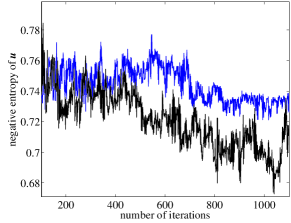
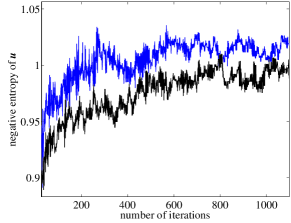
It is evident now that AdaBoost_ℓ1 controls the variance of margins by regularizing the Shannon entropy of the corresponding dual variable ${\boldsymbol{u}}$. For on-line learning algorithms there are two main families of regularization strategies: entropy regularization and regularization using squared Euclidean distance. A question that naturally arises here is: What happens if we use squared Euclidean distance to replace the entropy in the dual of AdaBoost_ℓ1 (3)? In other words, can we directly minimize the variance of the dual variable ${\boldsymbol{u}}$ to achieve the purpose of controlling the variance of margins? We answer this question by having a look at the convex loss functions for classification.

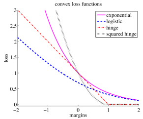
Fig. 2 plots four popular convex loss functions. It is shown in [26] that as the data size increases, practically all popular convex loss functions are Bayes-consistent, although convergence rates and other measures of consistency may vary. In the context of boosting, AdaBoost, LogitBoost and soft-margin LPBoost use exponential loss, logistic loss and hinge loss respectively. Here we are interested in the squared hinge loss. LogitBoost will be discussed in the next section. As mentioned, in theory, there is no particular reason to prefer hinge loss to squared hinge loss. Now if squared hinge loss is adopted, the cost function of soft-margin LPBoost (3.2) becomes

$$\mathop{\mathrm{max}}\limits_{{\boldsymbol{w}},\varrho,{\boldsymbol{\xi}}}~{}\varrho-D\textstyle\sum_{i=1}^{M}\xi_{i}^{2},$$

and the constraints remain the same as in (3.2). Its dual is easily derived

$$\mathop{\mathrm{min}}\limits_{r,{\boldsymbol{u}}}~{} r+\tfrac{1}{4D}{\textstyle\sum_{i=1}^{M}u_{i}^{2}}$$

$$\mathop{\mathrm{s.t.}}\nolimits~{} {\textstyle\sum_{i=1}^{M}}{u_{i}y_{i}H_{ij}}\leq r~{}(\forall j=1,\cdots,N),$$ (27)

$${\boldsymbol{u}}\succcurlyeq{\bf 0},{\bf 1}^{\!\top}{\boldsymbol{u}}=1.$$

We can view the above optimization problem as variance regularized LPBoost. In short, to minimize the variance of the dual variable ${\boldsymbol{u}}$ for controlling the margin’s variance, one can simply replace soft-margin LPBoost’s hinge loss with the squared hinge loss. Both the primal and dual problems are quadratic programs (QP) and hence can be efficiently solved using off-the-shelf QP solvers like Mosek [27], CPlex [28].

Actually we can generalize the hinge loss into

$$\left(\mathop{\mathrm{max}}\limits\{0,1-yF({\boldsymbol{x}})\}\right)^{p}.$$

When $p\geq 1$, the loss is convex. $p=1$ is the hinge loss and $p=2$ is the squared hinge loss. If we use a generalized hinge loss ($p>1$) for boosting, we end up with a regularized LPBoost which has the format:

$$\mathop{\mathrm{min}}\limits_{r,{\boldsymbol{u}}}~{}r+D^{1-q}(p^{1-q}-p^{-q}){\textstyle\sum_{i=1}^{M}u_{i}^{q}},$$ (28)

subject to the same constraints as in (3.3). Here $p$ and $q$ are dual to each other by $\frac{1}{p}+\frac{1}{q}=1$. It is interesting that (28) can also be seen as entropy regularized LPBoost; more precisely, Tsallis entropy [29] regularized LPBoost.

Definition 3.2

(Tsallis entropy) Tsallis entropy is a generalization of the Shannon entropy, defined as

$$S_{q}({\boldsymbol{u}})=\frac{1-\sum_{i}u_{i}^{q}}{q-1},~{}~{}({\boldsymbol{u}}\succcurlyeq 0,{\bf 1}^{\!\top}{\boldsymbol{u}}=1).$$ (29)

where $q$ is a real number. In the limit as $q\rightarrow 1$, we have $u_{i}^{q-1}=\exp((q-1)\log u_{i})\simeq 1+(q-1)\log u_{i}$. So $S_{1}=-\sum_{i}u_{i}\log u_{i}$, which is Shannon entropy.

Tsallis entropy [29] can also be viewed as a $q$-deformation of Shannon entropy because $S_{q}({\boldsymbol{u}})=-\sum_{i}u_{i}\log_{q}u_{i}$ where $\log_{q}(u)=\frac{u^{1-q}-1}{1-q}$ is the $q$-logarithm. Clearly $\log_{q}(u)\rightarrow\log(u)$ when $q\rightarrow 1$.

In summary, we conclude that although the primal problems of boosting with different loss functions seem dissimilar, their corresponding dual problems share the same formulation. Most of them can be interpreted as entropy regularized LPBoost. Table I summarizes the result. The analysis of LogitBoost will be presented in the next section.

TABLE I: Dual problems of boosting algorithms are entropy regularized LPBoost.

algorithm	loss in primal	entropy regularized LPBoost in dual
AdaBoost	exponential loss	Shannon entropy
LogitBoost	logistic loss	binary relative entropy
soft-margin $\ell_{p}(p>1)$ LPBoost	generalized hinge loss	Tsallis entropy

3.4 Lagrange dual of LogitBoost

Thus far, we have discussed AdaBoost and its relation to LPBoost. In this section, we consider LogitBoost [6] from its dual.

Theorem 3.2

The dual of LogitBoost is a binary relative entropy maximization problem, which writes

$$\mathop{\mathrm{max}}\limits_{r,{\boldsymbol{u}}}~{} \frac{r}{T}-{\textstyle\sum_{i=1}^{M}}\left[{(-u_{i})\log(-u_{i})}+(1+u_{i})\log(1+u_{i})\right]$$

$$\mathop{\mathrm{s.t.}}\nolimits~{} {\textstyle\sum_{i=1}^{M}}{u_{i}y_{i}H_{ij}}\geq r~{}(\forall j=1,\cdots,N).$$ (30)

We can also rewrite it into an equivalent form:

$$\mathop{\mathrm{min}}\limits_{r,{\boldsymbol{u}}}~{} r+T{\textstyle\sum_{i=1}^{M}}\left[{u_{i}\log u_{i}}+(1-u_{i})\log(1-u_{i})\right]$$

$$\mathop{\mathrm{s.t.}}\nolimits~{} {\textstyle\sum_{i=1}^{M}}{u_{i}y_{i}H_{ij}}\leq r~{}(\forall j=1,\cdots,N).$$ (31)

The proof follows the fact that the conjugate of the logistic loss function $\mathrm{logit}(x)=\log({1+\exp-x})$ is

$$\mathrm{logit}^{*}(u)=\begin{cases}(-u)\log(-u)+(1+u)\log(1+u),&\!\!\!\!\!0\geq u\geq-1;\\ \infty,&\!\!\!\!\!\text{otherwise},\end{cases}$$

with $0\log 0=0$. $\mathrm{logit}^{*}(u)$ is a convex function in its domain. The corresponding primal is

$$\min_{{\boldsymbol{w}}}~{} {\textstyle\sum_{i=1}^{M}}\mathrm{logit}(z_{i})$$

$$\mathop{\mathrm{s.t.}}\nolimits~{} z_{i}=y_{i}H_{i}{\boldsymbol{w}},~{}(\forall i=1,\cdots,M),$$ (32)

$${\boldsymbol{w}}\succcurlyeq{\bf 0},{\bf 1}^{\!\top}{\boldsymbol{w}}=\tfrac{1}{T}.$$

In (3.4), the dual variable ${\boldsymbol{u}}$ has a constraint ${\bf 1}\succcurlyeq{\boldsymbol{u}}\succcurlyeq{\bf 0}$, which is automatically enforced by the logarithmic function. Another difference of (3.4) from duals of AdaBoost and LPBoost etc. is that ${\boldsymbol{u}}$ does not need to be normalized. In other words, in LogitBoost the weight associated with each training sample is not necessarily a distribution. As in (24) for AdaBoost, we can also relate a dual optimal point ${\boldsymbol{u}}^{\star}$ and a primal optimal point ${\boldsymbol{w}}^{\star}$ ( between (3.4) and (3.4) ) by

$$u_{i}^{\star}=\frac{\exp-z_{i}^{\star}}{1+\exp-z_{i}^{\star}},\,\,\forall i=1,\cdots M.$$ (33)

So the margin of ${\boldsymbol{x}}_{i}$ is solely determined by $u_{i}^{\star}$: $z_{i}^{\star}=\log{\frac{1-u_{i}^{\star}}{u_{i}^{\star}}}$, $\forall i$. For a positive margin (${\boldsymbol{x}}_{i}$ is correctly classified), we must have $u_{i}^{\star}<0.5$.

Similarly, we can also use CG to solve LogitBoost. As shown in Algorithm LABEL:alg:AdaCG in the case of AdaBoost, the only modification is to solve a different dual problem (here we need to solve (3.4)).

3.5 AdaBoost_ℓ1 approximately maximizes the average margin and minimizes the margin variance

Before we present our main result, a lemma is needed.

Lemma 3.1

The margin of AdaBoost_ℓ1 and AdaBoost follows the Gaussian distribution. In general, the larger the number of weak classifiers, the more closely does the margin follow the form of Gaussian under the assumption that selected weak classifiers are uncorrelated.

• The central limit theorem [30] states that the sum of a set of i.i.d. random variables $x_{i}$, ($i=1\cdots N$) is approximately distributed following a Gaussian distribution if the random variables have finite mean and variance.

Figure 2: Various loss functions used in classification. Exponential: $\exp-s$; logistic: $\log(1+\exp-s)$; hinge: $\mathop{\mathrm{max}}\limits\{0,1-s\}$; squared hinge: $(\mathop{\mathrm{max}}\limits\{0,1-s\})^{2}$. Here $s=yF({\boldsymbol{x}})$.

Note that the central limit theorem applies when each variable $x_{i}$ has an arbitrary probability distribution ${\mathcal{Q}}_{i}$ as long as the mean and variance of ${\mathcal{Q}}_{i}$ are finite.

As mentioned, the normalized margin of AdaBoost for $i$-th example is defined as

$$\varrho_{i}=(y_{i}{\textstyle\sum_{j=1}^{N}h_{j}({\boldsymbol{x}}_{i})w_{j}})/{\bf 1}^{\!\top}{\boldsymbol{w}}=-z_{i}/{\bf 1}^{\!\top}{\boldsymbol{w}}.$$ (34)

In the following analysis, we ignore the normalization term ${\bf 1}^{\!\top}{\boldsymbol{w}}$ because it does not have any impact on the margin’s distribution. Hence the margin $\varrho$ is the sum of $N$ variables $\hat{w}_{j}$ with $\hat{w}_{j}=y_{i}h_{j}({\boldsymbol{x}}_{i})w_{j}$. It is easy to see that each $\hat{w}_{j}$ follows a discrete distribution with binary values either $w_{j}$ or $-w_{j}$. Therefore $w_{j}$ must have finite mean and variance. Using the central limit theorem, we know that the distribution of $\varrho_{i}$ is a Gaussian.

In the case of discrete variables ($\varrho_{i}$ can be discrete), the assumption identical distributions can be substantially weakened [31]. The generalized central limit theorem essentially states that anything that can be thought of as being made up as the sum of many small independent variables is approximately normally distributed.

A condition of the central limit theorem is that the $N$ variables must be independent. In the case of the number of weak hypotheses is finite, as the margin is expressed in (34), each $h_{j}(\cdot)$ is fixed beforehand, and assume all the training examples are randomly independently drawn, the variable $\varrho_{i}$ would be independent too. When the set of weak hypotheses is infinite, it is well known that usually AdaBoost selects independent weak classifiers such that each weak classifier makes different errors on the training dataset [15]. In this sense, $w_{j}$ might be viewed as roughly independent from each other. More diverse weak classifiers will make the selected weak classifiers less dependent.  ${\square}$

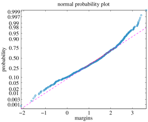
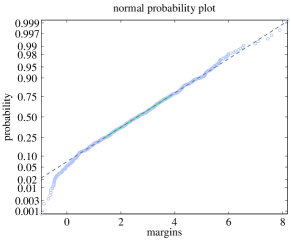
Here we give some empirical evidence for approximate Gaussianity. The normal (Gaussian) probability plot is used to visually assess whether the data follow a Gaussian distribution. If the data are Gaussian the plot forms a straight line. Other distribution types introduce curvature in the plot. We run AdaBoost with decision stumps on the dataset australian. Fig. 3 shows two plots of the margins with $50$ and $1100$ weak classifiers, respectively. We see that with $50$ weak classifiers, the margin distribution can be reasonably approximated by a Gaussian; with $1100$ classifiers, the distribution is very close to a Gaussian. The kurtosis of a 1D data provides a numerical evaluation of the Gaussianity. We know that the kurtosis of a Gaussian distribution is zero and almost all the other distributions have non-zero kurtosis. In our experiment, the kurtosis is $-0.056$ for the case with $50$ weak classifiers and $-0.34$ for $1100$ classifiers. Both are close to zero, which indicates AdaBoost’s margin distribution can be well approximated by Gaussian.

Figure 3: Gaussianity test for the margin distribution with $50$ and $1100$ weak classifiers, respectively. A Gaussian distribution will form a straight line. The dataset used is australian.

Theorem 3.3

AdaBoost_ℓ1 approximately maximizes the unnormalized average margin and at the same time minimizes the variance of the margin distribution under the assumption that the margin follows a Gaussian distribution.

• From (6) and (34), the cost function that AdaBoost_ℓ1 minimizes is

  $$f_{\mathrm{ab}}({\boldsymbol{w}})=\log\left({\textstyle\sum_{i=1}^{M}}\exp-\frac{\varrho_{i}}{T}\right).$$ (35)

  As proved in Lemma 3.1, $\varrho_{i}$ follows a Gaussian

  $${\mathcal{G}}(\varrho;{\bar{\varrho}},\sigma)={1\over\sqrt{2\pi}\sigma}\exp-\frac{(\varrho-{\bar{\varrho}})^{2}}{2\sigma^{2}},$$

  with mean ${\bar{\varrho}}$, variance $\sigma^{2}$; and $\sum_{i=1}^{M}\varrho_{i}=1$. We assume that the optimal value of the regularization parameter $T$ is known a priori.

  The Monte Carlo integration method can be used to compute a continuous integral

  $$\int g(x)f(x){\mathrm{d}}x\simeq\frac{1}{K}\sum_{k=1}^{K}f(x_{k}),$$ (36)

  where $g(x)$ is a probability distribution such that $\int g(x){\mathrm{d}}x=1$ and $f(x)$ is an arbitrary function. $x_{k}$, $(k=1\cdots K)$, are randomly sampled from the distribution $g(x)$. The more samples are used, the more accurate the approximation is.

  (35) can be viewed as a discrete Monte Carlo approximation of the following integral (we omit a constant term $\log M$, which is irrelevant to the analysis):

  $$\hat{f_{\mathrm{ab}}}({\boldsymbol{w}})$$

  $$=\log\int_{\varrho_{1}}^{\varrho_{2}}{\mathcal{G}}(\varrho;{\bar{\varrho}},\sigma)\exp\left(-\frac{\varrho}{T}\right){\mathrm{d}}\varrho$$

  $$=\log\int_{\varrho_{1}}^{\varrho_{2}}{1\over\sqrt{2\pi}\sigma}\exp\left(-\frac{(\varrho-{\bar{\varrho}})^{2}}{2\sigma^{2}}-\frac{\varrho}{T}\right){\mathrm{d}}\varrho$$

  $$=\log\left[\tfrac{1}{2}\exp\left(-\frac{{\bar{\varrho}}}{T}+\frac{\sigma^{2}}{2T^{2}}\right)\mathrm{erf}\left(\frac{\varrho-{\bar{\varrho}}}{\sqrt{2}\sigma}+\frac{\sigma}{\sqrt{2}T}\right)\bigg{|}_{\varrho_{1}}^{\varrho_{2}}\bigg{.}\right]$$

  $$=-\log 2-\frac{{\bar{\varrho}}}{T}+\frac{\sigma^{2}}{2T^{2}}+\log\left[\mathrm{erf}\left(\frac{\varrho-{\bar{\varrho}}}{\sqrt{2}\sigma}+\frac{\sigma}{\sqrt{2}T}\right)\bigg{|}_{\varrho_{1}}^{\varrho_{2}}\bigg{.}\right],$$ (37)

  where $\mathrm{erf}(x)=\frac{2}{\sqrt{\pi}}\int_{0}^{x}\exp-s^{2}{\mathrm{d}}s$ is the Gauss error function. The integral range is $[\varrho_{1},\varrho_{2}]$. With no explicit knowledge about the integration range, we may roughly calculate the integral from $-\infty$ to $+\infty$. Then the last term in (37) is $\log 2$ and the result is analytical and simple

  $$\hat{f_{\mathrm{ab}}}({\boldsymbol{w}})=-\frac{{\bar{\varrho}}}{T}+\frac{1}{2}\frac{\sigma^{2}}{T^{2}}.$$ (38)

  This is a reasonable approximation because Gaussian distributions drop off quickly (Gaussian is not considered a heavy-tailed distribution). Also this approximation implies that we are considering the case that the number of samples goes to $+\infty$.

Consequently, AdaBoost approximately maximizes the cost function

$$-\hat{f_{\mathrm{ab}}}({\boldsymbol{w}})=\frac{{\bar{\varrho}}}{T}-\frac{1}{2}\frac{\sigma^{2}}{T^{2}}.$$ (39)

This cost function has a clear and simple interpretation: The first term ${{\bar{\varrho}}}/{T}$ is the unnormalized average margin and the second term ${\sigma^{2}}/{T^{2}}$ is the unnormalized margin variance. So AdaBoost maximizes the unnormalized average margin and also takes minimizing the unnormalized margin variance into account. This way a better margin distribution can be obtained.  ${\square}$

Note that Theorem 3.3 depends on Lemma 3.1 that does not necessarily hold in practice.

Theorem 3.3 is an important result in the sense that it tries to contribute to the open question why AdaBoost works so well. Much previous work intends to believe that AdaBoost maximizes the minimum margin. We have theoretically shown that AdaBoost_ℓ1 optimizes the entire margin distribution by maximizing the mean and minimizing the variance of the margin distribution.

We notice that when $T\rightarrow 0$, Theorem 3.3 becomes invalid because the Monte Carlo integration cannot approximate the cost function of AdaBoost (35) well. In practice, $T$ cannot approach to zero arbitrarily in AdaBoost.

One may suspect that Theorem 3.3 contradicts the observation of similarity between LPBoost and AdaBoost as shown in Section 3.2. LPBoost maximizes the minimum margin and the dual of AdaBoost is merely an entropy regularized LPBoost. At first glance, the dual variable $r$ in (3), (3.2), and (3.2) should have the same meaning, i.e., maximum edge, which in turn corresponds to the minimum margin in the primal. Why average margin? To answer this question, let us again take a look at the optimality conditions. Let us denote the optimal values of (3) $r^{\star}$ and ${\boldsymbol{u}}^{\star}$. At convergence, we have $\frac{1}{T}(-r^{\star}+T\sum_{i=1}^{M}u_{i}^{\star}\log u_{i}^{\star})=\mathrm{Opt}_{(\ref{EQ:dual_ada0})}^{\star}=\mathrm{Opt}_{(\ref{EQ:2})}^{\star}=\mathrm{Opt}_{(\ref{EQ:2A})}^{\star}.$ Hence, we have

$$r^{\star}=T\sum_{i=1}^{M}u^{\star}\log u^{\star}-T\log\left(\sum_{i=1}^{M}\exp-\frac{\varrho_{i}^{\star}}{T}\right),$$

where $\varrho_{i}^{\star}$ is the normalized margin for ${\boldsymbol{x}}_{i}$. Clearly this is very different from the optimality conditions of LPBoost, which shows that $r^{\star}$ is the minimum margin. Only when $T\rightarrow 0$, the above relationship reduces to $r^{\star}=\mathop{\mathrm{min}}\limits_{i}\{\varrho_{i}^{\star}\}$—same as the case of LPBoost.

3.6 AdaBoost-QP: Direct optimization of the margin mean and variance using quadratic programming

The above analysis suggests that we can directly optimize the cost function (39). In this section we show that (39) is a convex programming (more precisely, quadratic programming, QP) problem in the variable ${\boldsymbol{w}}$ if we know all the base classifiers and hence it can be efficiently solved. Next we formulate the QP problem in detail. We call the proposed algorithm AdaBoost-QP.

In kernel methods like SVMs, the original space ${\mathcal{X}}$ is mapped to a feature space ${\mathcal{F}}$. The mapping function $\Phi(\cdot)$ is not explicitly computable. It is shown in [14] that in boosting, one can think of the mapping function $\Phi(\cdot)$ being explicitly known:

$$\Phi({\boldsymbol{x}}):{\boldsymbol{x}}\mapsto[h_{1}({\boldsymbol{x}}),\cdots,h_{N}({\boldsymbol{x}})]^{\!\top},$$ (40)

using the weak classifiers. Therefore, any weak classifier set ${\mathcal{H}}$ spans a feature space ${\mathcal{F}}$. We can design an algorithm that optimizes (39):

$$\mathop{\mathrm{min}}\limits_{\boldsymbol{w}}\,\,\tfrac{1}{2}{\boldsymbol{w}}^{\!\top}A{\boldsymbol{w}}-T{\boldsymbol{b}}^{\!\top}{\boldsymbol{w}},\,\,\,\,\mathop{\mathrm{s.t.}}\nolimits\,\,{\boldsymbol{w}}\succcurlyeq 0,{\bf 1}^{\!\top}{\boldsymbol{w}}=1,$$ (41)

where ${\boldsymbol{b}}=\frac{1}{M}\sum_{i=1}^{M}y_{i}H_{i}^{\!\top}=\frac{1}{M}\sum_{i=1}^{M}y_{i}\Phi({\boldsymbol{x}}_{i})$, and $A=\frac{1}{M}\sum_{i=1}^{M}(y_{i}H_{i}^{\!\top}-{\boldsymbol{b}})(y_{i}H_{i}^{\!\top}-{\boldsymbol{b}})^{\!\top}=\frac{1}{M}\sum_{i=1}^{M}(y_{i}\Phi({\boldsymbol{x}}_{i})-{\boldsymbol{b}})(y_{i}\Phi({\boldsymbol{x}}_{i})-{\boldsymbol{b}})^{\!\top}.$ Clearly $A$ must be positive semidefinite and this is a standard convex QP problem. The non-negativeness constraint ${\boldsymbol{w}}\succcurlyeq 0$ introduces sparsity as in SVMs. Without this constraint, the above QP can be analytically solved using eigenvalue decomposition—the largest eigenvector is the solution. Usually all entries of this solution would be active (non-zero values).

In the kernel space,

$${\boldsymbol{b}}^{\!\top}{\boldsymbol{w}}=\tfrac{1}{M}\left(\sum\nolimits_{y_{i}=1}\Phi({\boldsymbol{x}}_{i})-\sum\nolimits_{y_{i}=-1}\Phi({\boldsymbol{x}}_{i})\right)^{\!\top}{\boldsymbol{w}}$$

can be viewed as the projected $\ell_{1}$ norm distance between two classes because typically this value is positive assuming that each class has the same number of examples. The matrix $A$ approximately plays a role as the total scatter matrix in kernel linear discriminant analysis (LDA). Note that AdaBoost does not take the number of examples in each class into consideration when it models the problem. In contrast, LDA (kernel LDA) takes training example number into consideration. This may explain why an LDA post-processing on AdaBoost gives a better classification performance on face detection [33], which is a highly imbalanced classification problem. This observation of similarity between AdaBoost and kernel LDA may inspire new algorithms. We are also interested in developing a CG based algorithm for iteratively generating weak classifiers.

3.7 AdaBoost-CG: Totally corrective AdaBoost using column generation

The number of possible weak classifiers may be infinitely large. In this case it may be infeasible to solve the optimization exactly. AdaBoost works on the primal problem directly by switching between the estimating weak classifiers and computing optimal weights in a coordinate descent way. There is another method for working out of this problem by using an optimization technique termed column generation (CG) [34, 10]. CG mainly works on the dual problem. The basic concept of the CG method is to add one constraint at a time to the dual problem until an optimal solution is identified. More columns need to be generated and added to the problem to achieve optimality. In the primal space, the CG method solves the problem on a subset of variables, which corresponds to a subset of constraints in the dual. When a column is not included in the primal, the corresponding constraint does not appear in the dual. That is to say, a relaxed version of the dual problem is solved. If a constraint absent from the dual problem is violated by the solution to the restricted problem, this constraint needs to be included in the dual problem to further restrict its feasible region. In our case, instead of solving the optimization of AdaBoost directly, one computes the most violated constraint in (3) iteratively for the current solution and adds this constraint to the optimization problem. In theory, any column that violates dual feasibility can be added. To do so, we need to solve the following subproblem:

$$h^{\prime}(\cdot)=\mathop{\mathrm{argmax}}\limits_{h(\cdot)}~{}\textstyle\sum_{i=1}^{M}u_{i}y_{i}h({\boldsymbol{x}}_{i}).$$ (42)

This strategy is exactly the same as the one that stage-wise AdaBoost and LPBoost use for generating the best weak classifier. That is, to find the weak classifier that produces minimum weighted training error. Putting all the above analysis together, we summarize our AdaBoost-CG in Algorithm LABEL:alg:AdaCG.

The CG optimization (Algorithm LABEL:alg:AdaCG) is so general that it can be applied to all the boosting algorithms consider in this paper by solving the corresponding dual. The convergence follows general CG algorithms, which is easy to establish. When a new $h^{\prime}(\cdot)$ that violates dual feasibility is added, the new optimal value of the dual problem (maximization) would decrease. Accordingly, the optimal value of its primal problem decreases too because they have the same optimal value due to zero duality gap. Moreover the primal cost function is convex, therefore eventually it converges to the global minimum. A comment on the last step of Algorithm LABEL:alg:AdaCG is that we can get the value of ${\boldsymbol{w}}$ easily. Primal-dual interior-point (PD-IP) methods work on the primal and dual problems simultaneously and therefore both primal and dual variables are available after convergence. We use Mosek [27], which implements PD-IP methods. The primal variable ${\boldsymbol{w}}$ is obtained for free when solving the dual problem (3).

The dual subproblem we need to solve has one constraint added at each iteration. Hence after many iterations solving the dual problem could become intractable in theory. In practice, AdaBoost-CG converges quickly on our tested datasets. As pointed out in [35], usually only a small number of the added constraints are active and those inactive ones may be removed. This strategy prevents the dual problem from growing too large.

AdaBoost-CG is totally-corrective in the sense that the coefficients of all weak classifiers are updated at each iteration. In [36], an additional correction procedure is inserted to AdaBoost’s weak classifier selection cycle for achieving totally-correction. The inserted correction procedure aggressively reduces the upper bound of the training error. Like AdaBoost, it works in the primal. In contrast, our algorithm optimizes the regularized loss function directly and mainly works in the dual space. In [37], a totally-corrective boosting is proposed by optimizing the entropy, which is inspired by [18]. As discussed, no explicit primal-dual connection is established. That is why an LPBoost procedure is needed over the obtained weak classifiers in order to calculate the primal variable ${\boldsymbol{w}}$. In this sense, [37] is also similar to the work of [32].

Algorithm 2 AdaBoost-CG.

The following diagram summarizes the relationships that we have derived on the boosting algorithms that we have considered.

$$\begin{CD}\text{AdaBoost${}_{\ell 1}$ primal}@>{\text{{AdaBoost}-CG}}>{\text{Lagrange duality}}>\text{AdaBoost${}_{\ell 1}$ dual}\\ @V{\text{Theorem}~{}\ref{thm:4}}V{}V@A{\text{entropy}}A{\text{ regularization}}A\\ \text{{AdaBoost}-QP}\text{{LPBoost} dual}\\ \end{CD}$$

4 Experiments

In this section we provide experimental results to verify the presented theory. We have mainly used decision stumps as weak classifiers due to its simplicity and well-controlled complexity. In some cases, we have also used one of the simplest linear classifiers, LDA, as weak classifiers. To avoid the singularity problem when solving LDA, we add a scaled identity matrix $10^{-4}{\mathbf{I}}$ to the within-class matrix. For the CG optimization framework, we have confined ourself to AdaBoost-CG although the technique is general and applicable for optimizing other boosting algorithms.

4.1 AdaBoost-QP

We compare AdaBoost-QP against AdaBoost. We have used $14$ benchmark datasets [25]. Except mushrooms, svmguide1, svmguide3 and w1a, all the other datasets have been scaled to $[-1,1]$. We randomly split each dataset into training, cross-validation and test sets at a ratio of $70:15:15$.

The stopping criterion of AdaBoost is determined by cross-validation on $\{600,800,1000,1200,1500\}$ rounds of boosting. For AdaBoost-QP, the best value for the parameter $T$ is chosen from $\{\frac{1}{10},\frac{1}{20},\frac{1}{30},\frac{1}{40},\frac{1}{50},\frac{1}{100},\frac{1}{200},\frac{1}{500}\}$ by cross-validation. In this experiment, decision stumps are used as the weak classifier such that the complexity of the base classifiers is well controlled.

AdaBoost-QP must access all weak classifiers a priori. Here we run AdaBoost-QP on the $1500$ weak classifiers generated by AdaBoost. Clearly this number of hypotheses may not be optimal. Theoretically the larger the size of the weak classifier pool is, the better results AdaBoost-QP may produce. Table II reports the results. The experiments show that among these $14$ datasets, AdaBoost-QP outperforms AdaBoost on $9$ datasets in terms of generalization error. On mushrooms, both perform very well. On the other $4$ datasets, AdaBoost is better.

We have also computed the normalized version of the cost function value of (39). In most cases AdaBoost-QP has a larger value. This is not surprising since AdaBoost-QP directly maximizes (39) while AdaBoost approximately maximizes it. Furthermore, the normalized loss function value is close to the normalized average margin because the margin variances for most datasets are very small compared with their means.

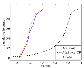
We also compute the largest minimum margin and average margin on each dataset. On all the datasets AdaBoost has a larger minimum margin than AdaBoost-QP, This confirms that the minimum margin is not crucial for the generalization error. On the other hand, the average margin produced by AdaBoost-QP, which is the first term of the cost function (39), is consistently larger than the one obtained by AdaBoost. Indirectly, we have shown that a better overall margin distribution is more important than the largest minimum margin. In Fig. 4 we plot cumulative margins for AdaBoost-QP and AdaBoost on the breast-cancer dataset with decision stumps. We can see that while Arc-Gv has a largest minimum margin, it has a worst margins distribution overall. If we examine the average margins, AdaBoost-QP is the largest; AdaBoost seconds and Arc-Gv is least. Clearly a better overall distribution does lead to a smaller generalization error. When Arc-Gv and AdaBoost run for more rounds, their margin distributions seem to converge. That is what we see in Fig. 4. These results agree well with our theoretical analysis (Theorem 3.3). Another observation from this experiment is that, to achieve the same performance, AdaBoost-QP tends to use fewer weak classifiers than AdaBoost does.

Figure 4: Cumulative margins for AdaBoost, AdaBoost-QP and Arc-Gv for the breast cancer dataset using decision stumps. Overall, the margin distribution of AdaBoost-QP is the best and it has a smallest test error. AdaBoost and Arc-Gv run $600$ rounds of boosting. Test error for AdaBoost, AdaBoost-QP and Arc-Gv is $0.029,0.027,0.058$ respectively.

We have also tested AdaBoost-QP on full sets of weak classifiers because the number of possible decision stumps is finite (less than (number of features $-1$) $\times$ (number of examples)). Table III reports the test error of AdaBoost-QP on some small datasets. As expected, in most cases, the test error is slightly better than the results using $1500$ decision stumps in Table II; and no significant difference is observed. This verifies the capability of AdaBoost-QP for selecting and combining relevant weak classifiers.

TABLE II: Test results of AdaBoost (AB) and AdaBoost-QP (QP). All tests are run $10$ times. The mean and standard deviation are reported. AdaBoost-QP outperforms AdaBoost on $9$ datasets.

dataset	algorithm	test error	minimum margin	average margin
australian	AB	$0.153\pm 0.034$	$\bf-0.012\pm 0.005$	$0.082\pm 0.006$
	QP	$\bf 0.13\pm 0.038$	$-0.227\pm 0.081$	$\bf 0.18\pm 0.052$
b-cancer	AB	$0.041\pm 0.013$	$\bf 0.048\pm 0.009$	$0.209\pm 0.02$
	QP	$\bf 0.03\pm 0.012$	$-0.424\pm 0.250$	$\bf 0.523\pm 0.237$
diabetes	AB	$0.270\pm 0.043$	$\bf-0.038\pm 0.007$	$0.055\pm 0.005$
	QP	$\bf 0.262\pm 0.047$	$-0.107\pm 0.060$	$\bf 0.075\pm 0.031$
fourclass	AB	$\bf 0.088\pm 0.032$	$\bf-0.045\pm 0.012$	$0.084\pm 0.009$
	QP	$0.095\pm 0.028$	$-0.211\pm 0.059$	$\bf 0.128\pm 0.027$
g-numer	AB	$0.283\pm 0.033$	$\bf-0.079\pm 0.017$	$0.042\pm 0.006$
	QP	$\bf 0.249\pm 0.033$	$-0.151\pm 0.058$	$\bf 0.061\pm 0.020$
heart	AB	$0.210\pm 0.032$	$\bf 0.02\pm 0.008$	$0.104\pm 0.013$
	QP	$\bf 0.190\pm 0.058$	$-0.117\pm 0.066$	$\bf 0.146\pm 0.059$
ionosphere	AB	$\bf 0.121\pm 0.044$	$\bf 0.101\pm 0.010$	$0.165\pm 0.012$
	QP	$0.139\pm 0.055$	$-0.035\pm 0.112$	$\bf 0.184\pm 0.063$
liver	AB	$0.321\pm 0.040$	$\bf-0.012\pm 0.007$	$0.055\pm 0.005$
	QP	$\bf 0.314\pm 0.060$	$-0.107\pm 0.044$	$\bf 0.079\pm 0.021$
mushrooms	AB	$\bf 0\pm 0$	$\bf 0.102\pm 0.001$	$0.181\pm 0.001$
	QP	$0.005\pm 0.002$	$-0.134\pm 0.086$	$\bf 0.221\pm 0.084$
sonar	AB	$\bf 0.145\pm 0.046$	$\bf 0.156\pm 0.008$	$0.202\pm 0.013$
	QP	$0.171\pm 0.048$	$0.056\pm 0.066$	$\bf 0.220\pm 0.045$
splice	AB	$0.129\pm 0.025$	$\bf-0.009\pm 0.008$	$0.117\pm 0.009$
	QP	$\bf 0.106\pm 0.029$	$-0.21\pm 0.037$	$\bf 0.189\pm 0.02$
svmguide1	AB	$\bf 0.035\pm 0.009$	$\bf-0.010\pm 0.008$	$0.157\pm 0.016$
	QP	$0.040\pm 0.009$	$-0.439\pm 0.183$	$\bf 0.445\pm 0.155$
svmguide3	AB	$0.172\pm 0.023$	$\bf-0.011\pm 0.009$	$0.052\pm 0.005$
	QP	$\bf 0.167\pm 0.022$	$-0.113\pm 0.084$	$\bf 0.085\pm 0.038$
w1a	AB	$0.041\pm 0.014$	$\bf-0.048\pm 0.010$	$0.084\pm 0.005$
	QP	$\bf 0.029\pm 0.009$	$-0.624\pm 0.38$	$\bf 0.577\pm 0.363$

TABLE III: Test results of AdaBoost-QP on full sets of decision stumps. All tests are run $10$ times.

dataset	australian	b-cancer	fourclass	g-numer	heart	liver	mushroom	splice
test error	$0.131\pm 0.041$	$0.03\pm 0.011$	$0.091\pm 0.02$	$0.243\pm 0.026$	$0.188\pm 0.058$	$0.319\pm 0.05$	$0.003\pm 0.001$	$0.097\pm 0.02$

4.2 AdaBoost-CG

We run AdaBoost and AdaBoost-CG with decision stumps on the datasets of [25]. $70\%$ of examples are used for training; $15\%$ are used for test and the other $15\%$ are not used because we do not do cross-validation here. The convergence threshold for AdaBoost-CG ($\varepsilon$ in Algorithm LABEL:alg:AdaCG) is set to $10^{-5}$. Another important parameter to tune is the regularization parameter $T$. For the first experiment, we have set it to $1/{\bf 1}^{\!\top}{\boldsymbol{w}}$ where ${\boldsymbol{w}}$ is obtained by running AdaBoost on the same data for $1000$ iterations. Also for fair comparison, we have deliberately forced AdaBoost-CG to run $1000$ iterations even if the stopping criterion is met. Both test and training results for AdaBoost and AdaBoost-CG are reported in Table IV for a maximum number of iterations of $100$, $500$ and $1000$.

As expected, in terms of test error, no algorithm statistically outperforms the other one, since they optimize the same cost function. As we can see, AdaBoost does slightly better on $6$ datasets. AdaBoost-CG outperforms AdaBoost on $7$ datasets and on svmguide1, both algorithms perform almost identically. Therefore, empirically we conclude that in therms of generalization capability, AdaBoost-CG is the same as the standard AdaBoost.

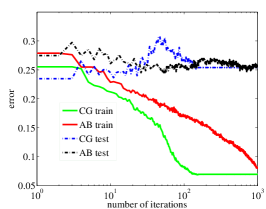
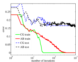
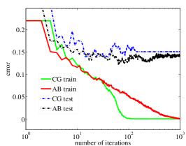
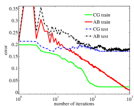
However, in terms of training error and convergence speed of the training procedure, there is significant difference between these two algorithms. Looking at the right part of Table IV, we see that the training error of AdaBoost-CG is consistently better or no worse than AdaBoost on all tested datasets. We have the following conclusions.

• The convergence speed of AdaBoost-CG is faster than AdaBoost and in many cases, better training error can be achieved. This is because AdaBoost’s coordinate descent nature is slow while AdaBoost-CG is totally corrective. This also means that with AdaBoost-CG, we can use fewer weak classifiers to build a good strong classifier. This is desirable for real-time applications like face detection [38], in which the testing speed is critical.

• Our experiments confirm that a smaller training error does not necessarily lead to a smaller test error. This has been studied extensively in statistical learning theory. It is observed that AdaBoost sometimes suffers from overfitting and minimizing the exponential cost function of the margins does not solely determine test error.

In the second experiment, we run cross-validation to select the best value for the regularization parameter $T$, same as in Section 4.1. Table V reports the test errors on a subset of the datasets. Slightly better results are obtained compared with the results in Table IV, which uses $T$ determined by AdaBoost.

TABLE IV: Test and training errors of AdaBoost (AB) and AdaBoost-CG (CG). All tests are run $5$ times. The mean and standard deviation are reported. Weak classifiers are decision stumps.

dataset	algorithm	test error $100$	test error $500$	test error $1000$	train error $100$	train error $500$	train error $1000$
australian	AB	$\bf 0.146\pm 0.028$	$\bf 0.165\pm 0.018$	$\bf 0.163\pm 0.021$	$0.091\pm 0.013$	$0.039\pm 0.011$	$0.013\pm 0.009$
	CG	$0.177\pm 0.025$	$0.167\pm 0.023$	$0.167\pm 0.023$	$\bf 0.013\pm 0.008$	$\bf 0.011\pm 0.007$	$\bf 0.011\pm 0.007$
b-cancer	AB	$\bf 0.041\pm 0.026$	$\bf 0.045\pm 0.030$	$\bf 0.047\pm 0.032$	$0.008\pm 0.006$	$0\pm 0$	$0\pm 0$
	CG	$0.049\pm 0.033$	$0.049\pm 0.033$	$0.049\pm 0.033$	$\bf 0\pm 0$	$0\pm 0$	$0\pm 0$
diabetes	AB	$\bf 0.254\pm 0.024$	$0.263\pm 0.028$	$0.257\pm 0.041$	$0.171\pm 0.012$	$0.120\pm 0.007$	$0.082\pm 0.006$
	CG	$0.270\pm 0.047$	$\bf 0.254\pm 0.026$	$\bf 0.254\pm 0.026$	$\bf 0.083\pm 0.008$	$\bf 0.070\pm 0.007$	$\bf 0.070\pm 0.007$
fourclass	AB	$0.106\pm 0.047$	$0.097\pm 0.034$	$0.091\pm 0.031$	$0.072\pm 0.023$	$0.053\pm 0.017$	$0.046\pm 0.017$
	CG	$\bf 0.082\pm 0.031$	$\bf 0.082\pm 0.031$	$\bf 0.082\pm 0.031$	$\bf 0.042\pm 0.015$	$\bf 0.042\pm 0.015$	$\bf 0.042\pm 0.015$
g-numer	AB	$0.279\pm 0.043$	$0.288\pm 0.048$	$0.297\pm 0.051$	$0.206\pm 0.047$	$0.167\pm 0.072$	$0.155\pm 0.082$
	CG	$\bf 0.269\pm 0.040$	$\bf 0.262\pm 0.045$	$\bf 0.262\pm 0.045$	$\bf 0.142\pm 0.077$	$\bf 0.142\pm 0.077$	$\bf 0.142\pm 0.077$
heart	AB	$0.175\pm 0.073$	$0.175\pm 0.088$	$0.165\pm 0.076$	$0.049\pm 0.022$	$0\pm 0$	$0\pm 0$
	CG	$\bf 0.165\pm 0.072$	$\bf 0.165\pm 0.072$	$\bf 0.165\pm 0.072$	$\bf 0\pm 0$	$0\pm 0$	$0\pm 0$
ionosphere	AB	$\bf 0.092\pm 0.016$	$\bf 0.104\pm 0.017$	$\bf 0.100\pm 0.016$	$0\pm 0$	$0\pm 0$	$0\pm 0$
	CG	$0.131\pm 0.034$	$0.131\pm 0.034$	$0.131\pm 0.034$	$0\pm 0$	$0\pm 0$	$0\pm 0$
liver	AB	$0.288\pm 0.101$	$\bf 0.265\pm 0.081$	$\bf 0.281\pm 0.062$	$0.144\pm 0.018$	$0.063\pm 0.015$	$0.020\pm 0.015$
	CG	$\bf 0.288\pm 0.084$	$0.288\pm 0.084$	$0.288\pm 0.084$	$\bf 0.017\pm 0.012$	$\bf 0.017\pm 0.011$	$\bf 0.017\pm 0.011$
mushrooms	AB	$0\pm 0.001$	$0\pm 0.001$	$0\pm 0$	$0\pm 0$	$0\pm 0$	$0\pm 0$
	CG	$\bf 0\pm 0$	$\bf 0\pm 0$	$0\pm 0$	$0\pm 0$	$0\pm 0$	$0\pm 0$
sonar	AB	$\bf 0.206\pm 0.087$	$\bf 0.213\pm 0.071$	$\bf 0.206\pm 0.059$	$0\pm 0$	$0\pm 0$	$0\pm 0$
	CG	$0.232\pm 0.053$	$0.245\pm 0.078$	$0.245\pm 0.078$	$0\pm 0$	$0\pm 0$	$0\pm 0$
splice	AB	$\bf 0.129\pm 0.011$	$\bf 0.143\pm 0.026$	$\bf 0.143\pm 0.020$	$0.053\pm 0.003$	$0.008\pm 0.006$	$0.001\pm 0.001$
	CG	$0.161\pm 0.033$	$0.151\pm 0.023$	$0.151\pm 0.023$	$\bf 0.002\pm 0.002$	$\bf 0.001\pm 0.002$	$\bf 0.001\pm 0.002$
svmguide1	AB	$\bf 0.036\pm 0.012$	$\bf 0.034\pm 0.008$	$0.037\pm 0.007$	$0.022\pm 0.002$	$0.009\pm 0.002$	$0.002\pm 0.001$
	CG	$0.037\pm 0.007$	$0.037\pm 0.007$	$0.037\pm 0.007$	$\bf 0.001\pm 0.001$	$\bf 0\pm 0.001$	$\bf 0\pm 0.001$
svmguide3	AB	$0.184\pm 0.037$	$0.183\pm 0.044$	$0.182\pm 0.031$	$0.112\pm 0.009$	$0.037\pm 0.004$	$0.009\pm 0.003$
	CG	$\bf 0.184\pm 0.026$	$\bf 0.171\pm 0.023$	$\bf 0.171\pm 0.023$	$\bf 0.033\pm 0.012$	$\bf 0.023\pm 0.016$	$\bf 0.023\pm 0.016$
w1a	AB	$0.051\pm 0.009$	$0.038\pm 0.005$	$0.036\pm 0.004$	$0.045\pm 0.008$	$0.028\pm 0.005$	$0.025\pm 0.005$
	CG	$\bf 0.018\pm 0.001$	$\bf 0.018\pm 0.001$	$\bf 0.018\pm 0.001$	$\bf 0.010\pm 0.004$	$\bf 0.010\pm 0.004$	$\bf 0.010\pm 0.004$

Figure 5: Test error and training error of AdaBoost, AdaBoost-CG for australian, breast-cancer, diabetes, heart, spline and svmguide3 datasets. These convergence curves correspond to the results in Table IV. The $x$-axis is on a logarithmic scale for easier comparison.

TABLE V: Test error of AdaBoost-CG with decision stumps, using cross-validation to select the optimal $T$. All tests are run $5$ times.

dataset	australian	b-cancer	diabetes	fourclass	heart	ionosphere	sonar	splice
test error	$0.146\pm 0.027$	$0.033\pm 0.033$	$0.266\pm 0.036$	$0.086\pm 0.027$	$0.17\pm 0.082$	$0.115\pm 0.024$	$0.2\pm 0.035$	$0.135\pm 0.015$

We also use LDA as weak classifiers to compare the classification performance of AdaBoost and AdaBoost-CG. The parameter $T$ of AdaBoost-CG is determined by cross-validation from $\{$$\frac{1}{2},$ $\frac{1}{5},$ $\frac{1}{8},$ $\frac{1}{10},$ $\frac{1}{12},$ $\frac{1}{15},$ $\frac{1}{20},$ $\frac{1}{30},$ $\frac{1}{40},$ $\frac{1}{50},$ $\frac{1}{70},$ $\frac{1}{90},$ $\frac{1}{100},$ $\frac{1}{120},$ $\frac{1}{150}$$\}$. For AdaBoost the smallest test error from $100$, $500$ and $1000$ runs is reported. We show the results in Table VI. As we can see, the test error is slightly better than with decision stumps for both AdaBoost and AdaBoost-CG. Again, AdaBoost and AdaBoost-CG’s performances are very similar.

In order to show that statistically there are no difference between AdaBoost-CG and AdaBoost, the McNemar test [39] with the significance level of $0.05$ is conducted. McNemar’s test is based on a $\chi^{2}$ test [39]. If the quantity of the $\chi^{2}$ test is not greater than $\chi^{2}_{1,0.95}=3.841459$, we can think of that the two tested classifiers have no statistical difference in terms of classification capability. On the $8$ datasets with decision stumps and LDA (Tables V and VI), in all cases ($5$ runs per dataset), the results of $\chi^{2}$ test are smaller than $\chi^{2}_{1,0.95}$. Consequently, we can conclude that indeed AdaBoost-CG performs very similarly to AdaBoost for classification.

TABLE VI: Test error of AdaBoost (AB) and AdaBoost-CG (CG) with LDA as weak classifiers, using cross-validation to select the optimal $T$. All tests are run $5$ times.

dataset	australian	b-cancer	diabetes	fourclass	heart	ionosphere	sonar	splice
AB	$0.150\pm 0.044$	$0.029\pm 0.014$	$0.259\pm 0.021$	$0.003\pm 0.004$	$0.16\pm 0.055$	$0.108\pm 0.060$	$0.297\pm 0.080$	$0.215\pm 0.027$
CG	$0.151\pm 0.053$	$0.035\pm 0.016$	$0.249\pm 0.038$	$0.022\pm 0.015$	$0.185\pm 0.038$	$0.104\pm 0.062$	$0.258\pm 0.085$	$0.235\pm 0.035$

To examine the effect of parameter $T$, we run more experiments with various $T$ on the banana dataset (2D artificial data) that was used in [32]. We still use decision stumps. The maximum iteration is set to $400$. All runs stop earlier than $100$ iterations. Table VII reports the results. Indeed, the training error depends on $T$. $T$ also has influence on the convergence speed. But, in a wide range of $T$, the test error does not change significantly. We do not have a sophisticated technique to tune $T$. As mentioned, the sum of ${\boldsymbol{w}}$ from a run of AdaBoost can serve as a heuristic.

TABLE VII: AdaBoost-CG on banana dataset with decision stumps and LDA as weak classifiers. Experiments are run $50$ times.

$\frac{1}{T}$	test (stumps)	train (stumps)	test (LDA)	train (LDA)
$20$	$0.298\pm 0.018$	$0.150\pm 0.019$	$0.134\pm 0.012$	$0.032\pm 0.007$
$40$	$0.309\pm 0.019$	$0.101\pm 0.015$	$0.135\pm 0.008$	$0.001\pm 0.002$
$80$	$0.313\pm 0.019$	$0.033\pm 0.011$	$0.136\pm 0.007$	$0\pm 0$

TABLE VIII: Test error of LogitBoost-CG with decision stumps, using cross-validation to select the optimal $T$. All tests are run $5$ times.

dataset	australian	b-cancer	diabetes	fourclass	heart	ionosphere	sonar	splice
test error	$0.13\pm 0.043$	$0.039\pm 0.012$	$0.238\pm 0.057$	$0.071\pm 0.034$	$0.14\pm 0.095$	$0.2\pm 0.069$	$0.169\pm 0.05$	$0.104\pm 0.021$

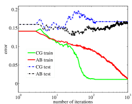
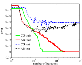
Now let us take a close look at the convergence behavior of AdaBoost-CG. Fig. 5 shows the test and training error of AdaBoost and AdaBoost-CG for $6$ datasets. We see that AdaBoost-CG converges much faster than AdaBoost in terms of number of iterations. On most tested datasets, AdaBoost-CG is around $10$ times faster than AdaBoost. The test error for these two methods are very close upon convergence. In some datasets such as australian and breast-cancer we observe over-fitting for AdaBoost.

4.3 LogitBoost-CG

We have also run LogitBoost-CG on the same datasets. All the settings are the same as in the case of AdaBoost-CG. The weak classifiers are decision stumps. Table VIII reports the experiment results. Compared to Table V, very similar results have been observed. No one achieves better results over the other one on all the datasets.

5 Discussion and Conclusion

In this paper, we have shown that the Lagrange dual problems of AdaBoost, LogitBoost and soft-margin LPBoost with generalized hinge loss are all entropy regularized LPBoost. We both theoretically and empirically demonstrate that the success of AdaBoost relies on maintaining a better margin distribution. Based on the dual formulation, a general column generation based optimization framework is proposed. This optimization framework can be applied to solve all the boosting algorithms with various loss functions mentioned in this paper. Experiments with exponential loss show that the classification performance of AdaBoost-CG is statistically almost identical to the standard stage-wise AdaBoost on real datasets. In fact, since both algorithms optimize the same cost function, we would be surprised to see a significant different in their generalization error. The main advantage of the proposed algorithms is significantly faster convergence speed.

Compared with the conventional AdaBoost, a drawback of AdaBoost-CG is the introduction of a parameter, same as in LPBoost. While one can argue that AdaBoost implicitly determines this same parameter by selecting how many iterations to run, the stopping criterion is nested and thus efficient to learn. In the case of AdaBoost-CG, it is not clear how to efficiently learn this parameter. Currently, one has to run the training procedure multiple times for cross validation.

With the optimization framework established here, some issues on boosting that are previously unclear may become obvious now. For example, for designing cost-sensitive boosting or boosting on uneven datasets, one can simply modify the primal cost function (5) to have a weighted cost function [40]. The training procedure follows AdaBoost-CG.

To summarize, the convex duality of boosting algorithms presented in this work generalizes the convex duality in LPBoost. We have shown some interesting properties that the derived dual formation possesses. The duality also leads to new efficient learning algorithms. The duality provides useful insights on boosting that may lack in existing interpretations [2, 6].

In the future, we want to extend our work to boosting with non-convex loss functions such as BrownBoost [41]. Also it should be straightforward to optimize boosting for regression using column generation. We are currently exploring the application of AdaBoost-CG to efficient object detection due to its faster convergence, which is more promising for feature selection [38].

Appendix A Description of datasets

TABLE IX: Description of the datasets. Except mushrooms, svmguide1, svmguide3 and w1a, all the other datasets have been scaled to $[-1,1]$.

dataset	# examples	# features	dataset	# examples	# features
australian	690	14	liver-disorders	345	6
breast-cancer	683	10	mushrooms	8124	112
diabetes	768	8	sonar	208	60
fourclass	862	2	splice	1000	60
german-numer	1000	24	svmguide1	3089	4
heart	270	13	svmguide3	1243	22
ionosphere	351	34	w1a	2477	300

Table IX provides a description of the datasets we have used in the experiments.

References

- [1] Y. Freund and R. E. Schapire, “A decision-theoretic generalization of on-line learning and an application to boosting,” J. Comp. & Syst. Sci., vol. 55, no. 1, pp. 119–139, 1997.
- [2] R. E. Schapire, Y. Freund, P. Bartlett, and W. S. Lee, “Boosting the margin: A new explanation for the effectiveness of voting methods,” Ann. Statist., vol. 26, no. 5, pp. 1651–1686, 1998.
- [3] C. Rudin, I. Daubechies, and R. E. Schapire, “The dynamics of AdaBoost: Cyclic behavior and convergence of margins,” J. Mach. Learn. Res., vol. 5, pp. 1557–1595, 2004.
- [4] C. Rudin, R. E. Schapire, and I. Daubechies, “Analysis of boosting algorithms using the smooth margin function,” Ann. Statist., vol. 35, no. 6, pp. 2723–2768, 2007.
- [5] D. Mease and A. Wyner, “Evidence contrary to the statistical view of boosting,” J. Mach. Learn. Res., vol. 9, pp. 131–156, 2008.
- [6] J. Friedman, T. Hastie, and R. Tibshirani, “Additive logistic regression: a statistical view of boosting (with discussion and a rejoinder by the authors),” Ann. Statist., vol. 28, no. 2, pp. 337–407, 2000.
- [7] C. Domingo and O. Watanabe, “MadaBoost: A modification of AdaBoost,” in Proc. Annual Conf. Learn. Theory. 2000, pp. 180–189, Morgan Kaufmann.
- [8] G. Rätsch and M. K. Warmuth, “Efficient margin maximizing with boosting,” J. Mach. Learn. Res., vol. 6, pp. 2131–2152, 2005.
- [9] A. J. Grove and D. Schuurmans, “Boosting in the limit: maximizing the margin of learned ensembles,” in Proc. National Conf. Artificial Intell., Madison, Wisconsin, USA, 1998, pp. 692–699.
- [10] A. Demiriz, K.P. Bennett, and J. Shawe-Taylor, “Linear programming boosting via column generation,” Mach. Learn., vol. 46, no. 1-3, pp. 225–254, 2002.
- [11] L. Breiman, “Prediction games and arcing algorithms,” Neural Comp., vol. 11, no. 7, pp. 1493–1517, 1999.
- [12] L. Reyzin and R. E. Schapire, “How boosting the margin can also boost classifier complexity,” in Proc. Int. Conf. Mach. Learn., Pittsburgh, Pennsylvania, USA, 2006.
- [13] V. Koltchinskii and D. Panchenko, “Empirical margin distributions and bounding the generalization error of combined classifiers,” Ann. Statist., vol. 30, no. 1, pp. 1–50, 2002.
- [14] G. Rätsch, S. Mika, B. Schölkopf, and K.-R. Müller, “Constructing boosting algorithms from SVMs: An application to one-class classification,” IEEE Trans. Pattern Anal. Mach. Intell., vol. 24, no. 9, pp. 1184–1199, 2002.
- [15] R. Meir and G. Rätsch, An introduction to boosting and leveraging, pp. 118–183, Advanced lectures on machine learning. Springer-Verlag, New York, NY, USA, 2003.
- [16] R. E. Schapire, The boosting approach to machine learning: An overview, pp. 149–172, Nonlinear Estimation and Classification. Springer, 2003.
- [17] M. Collins, R. E. Schapire, and Y. Singer, “Logistic regression, AdaBoost and Bregman distances,” Mach. Learn., vol. 48, no. 1-3, pp. 253–285, 2002.
- [18] J. Kivinen and M. K. Warmuth, “Boosting as entropy projection,” in Proc. Annual Conf. Learn. Theory, Santa Cruz, California, US, 1999, pp. 134–144, ACM.
- [19] G. Lebanon and J. Lafferty, “Boosting and maximum likelihood for exponential models,” in Proc. Adv. Neural Inf. Process. Syst. 2001, pp. 447–454, MIT Press.
- [20] L. Mason, J. Baxter, P. Bartlett, and M. Frean, Functional gradient techniques for combining hypotheses, chapter 12, pp. 221–247, Advances in Large Margin Classifiers. MIT press, 1999.
- [21] S. Boyd and L. Vandenberghe, Convex Optimization, Cambridge University Press, 2004.
- [22] Y. Freund and R. E. Schapire, “Adaptive game playing using multiplicative weights,” Games & Economic Behavior, vol. 29, pp. 79–103, 1999.
- [23] R. M. Rifkin and R. A. Lippert, “Value regularization and Fenchel duality,” J. Mach. Learn. Res., vol. 8, pp. 441–479, 2007.
- [24] S. Shalev-Shwartz and Y. Singer, “On the equivalence of weak learnability and linear separability: New relaxations and efficient boosting algorithms,” in Proc. Annual Conf. Learn. Theory, Helsinki, Finland, 2008.
- [25] C.-C. Chang and C.-J. Lin, “LIBSVM: a library for support vector machines,” 2001, http://www.csie.ntu.edu.tw/cjlin/libsvmtools/datasets/.
- [26] P. Bartlett, M. Jordan, and J. McAuliffe, “Convexity, classification, and risk bounds,” J. Amer. Stat. Assoc., vol. 101, no. 473, pp. 138–156, 2004.
- [27] MOSEK ApS, “The MOSEK optimization toolbox for matlab manual, version 5.0, revision 93,” 2008, http://www.mosek.com/.
- [28] ILOG, Inc., “CPLEX 11.1,” 2008, http://www.ilog.com/products/cplex/.
- [29] C. Tsallis, “Possible generalization of Boltzmann-Gibbs statistics,” J. Stat. Physics, vol. 52, pp. 479–487, 1988.
- [30] O. Kallenberg, Foundations of Modern Probability, Springer-Verlag, 1997.
- [31] W. Feller, Introduction to Probability Theory and its Applications, 3rd Ed., vol. 1, John Wiley & Sons, 1968.
- [32] G. Rätsch, T. Onoda, and K.-R. Müller, “Soft margins for AdaBoost,” Mach. Learn., vol. 42, no. 3, pp. 287–320, 2001, data sets are available at http://theoval.cmp.uea.ac.uk/~gcc/matlab/index.shtml.
- [33] J. Wu, M. D. Mullin, and J. M. Rehg, “Linear asymmetric classifier for cascade detectors,” in Proc. Int. Conf. Mach. Learn., Bonn, Germany, 2005, pp. 988–995.
- [34] M. E. Lübbecke and J. Desrosiers, “Selected topics in column generation,” Operation Res., vol. 53, no. 6, pp. 1007–1023, 2005.
- [35] S. Sonnenburg, G. Rätsch, C. Schäfer, and B. Schölkopf, “Large scale multiple kernel learning,” J. Mach. Learn. Res., vol. 7, pp. 1531–1565, 2006.
- [36] J. S̆ochman and J. Malas, “AdaBoost with totally corrective updates for fast face detection,” in Proc. IEEE Int. Conf. Automatic Face & Gesture Recogn., Seoul, Korea, 2004, pp. 445–450.
- [37] M. K. Warmuth, J. Liao, and G. Rätsch, “Totally corrective boosting algorithms that maximize the margin,” in Proc. Int. Conf. Mach. Learn., Pittsburgh, Pennsylvania, 2006, pp. 1001–1008.
- [38] P. Viola and M. J. Jones, “Robust real-time face detection,” Int. J. Comp. Vis., vol. 57, no. 2, pp. 137–154, 2004.
- [39] T. G. Dietterich, “Approximate statistical tests for comparing supervised classification learning algorithms,” Neural Comp., vol. 10, no. 7, pp. 1895–1923, 1998.
- [40] J. Leskovec, “Linear programming boosting for uneven datasets,” in Proc. Int. Conf. Mach. Learn., 2003, pp. 456–463.
- [41] Y. Freund, “An adaptive version of the boost by majority algorithm,” Mach. Learn., vol. 43, no. 3, pp. 293–318, 2001.