Hysteresis and noise in ferromagnetic materials with parallel domain walls

Abstract

We investigate dynamic hysteresis and Barkhausen noise in ferromagnetic materials with a huge number of parallel and rigid Bloch domain walls. Considering a disordered ferromagnetic system with strong in-plane uniaxial anisotropy and in-plane magnetization driven by an external magnetic field, we calculate the equations of motion for a set of coupled domain walls, considering the effects of the long-range dipolar interactions and disorder. We derive analytically an expression for the magnetic susceptivity, related to the effective demagnetizing factor, and show that it has a logarithmic dependence on the number of domains. Next, we simulate the equations of motion and study the effect of the external field frequency and the disorder on the hysteresis and noise properties. The dynamic hysteresis is very well explained by means of the loss separation theory.

I introduction

The study of ferromagnetic hysteresis represents an open field of current interest, due to the applications in magnetic recording technology and spintronic devices bertotti . From a purely theoretical point of view, the dynamics of disordered magnetic systems represents a central problem in non-equilibrium statistical mechanics. One of the central questions arising in the analysis of ferromagnetic systems, is the link between the domain structure and the hysteretic properties, such as the coercive field, the power losses and the noise. From the experimental point of view, it is possible to observe the domain structure on the surface of the sample by magneto-optical techniques, while the bulk behavior is accessible by inductive techniques. Several models have been developed to understand the experimental results, ranging from Ising type models considering the reversal of a set of interacting spins with RFIM ; sethna ; vives ; vives2 ; vives3 or without disorder chakrabarti ; acharyya ; sides ; rikvold ; rikvold1 , to models focusing on the dynamics of a single domain wall lyuksyutov ; ABBM ; zapperi ; zapperi2 ; urbach ; narayan ; bahiana ; queiroz . These two classes of models represent two extreme situations: spin models are appropriate when dipolar interactions are negligible. On the other hand, in soft magnetic materials magnetostatic effects induce wide parallel domain walls that determine the magnetization properties.

The dependence of the hysteresis loop area on the frequency and the amplitude of the applied magnetic field is often referred to as dynamic hysteresis chakrabarti ; moore in the context of thin films and to power losses in bulk materials. In bulk materials, energy dissipation is dominated by eddy currents propagation bertotti , while in thin films this effect is negligible. This led to the general belief that dynamic hysteresis in thin films is ruled by completely different laws than in bulk samples. The results of the models used to analyze dynamic hysteresis are often interpreted by assuming a universal scaling law for the dependence of hysteresis loop area $A$ on the temperature of the system $T$, the applied field frequency $\omega$ and amplitude $H_{0}$. The experimental estimates of the scaling exponents display a huge variability he ; luse ; jiang ; raquet ; suen ; bland1 ; choi ; lee2 ; lee3 ; suen2 , and the validity of a universal scaling law is still under debate santi ; nistor . In this respect, it was recently shown that the theory of loss separation developed for bulk materials could be equally well applied to thin films, since the precise nature of the damping (i.e. eddy currents or spin relaxation) does not change the basic equations colaiori .

The Barkhausen effect barkhausen consists in the irregularity of the magnetization variation while magnetizing a sample with a slowly varying external magnetic field. It is due to the jerky motion of the domain walls in a system with structural disorder and impurities BK . Once the origin of Barkhausen noise (BN) was understood wisho , it was soon realized that it could be used as a non-destructive and non-invasive probe to investigate the magnetization dynamics in magnetic materials. From a theoretical point of view, it is a good example of dynamical critical behavior, as evidenced by experimental observations of power law distributions for the statistics of the avalanche size and duration sethna . There is a growing evidence that soft magnetic bulk materials can be grouped into different classes according to the scaling exponents values dz . The Barkhausen noise is also an example of dynamics of a system presenting collective pinning when a quenched disorder is present, and it belongs to the family of the so-called crackling noises sethna . This kind of noise is exhibited by a wide variety of physical systems, from earthquakes on faults to paper crumpling. So the relative ease to study crackling noise in magnets make the BN useful to get a deeper insight on different complex systems.

The most successful models used to describe the BN have considered the dynamics of a single domain wall lyuksyutov ; ABBM ; zapperi ; zapperi2 ; urbach ; narayan ; bahiana ; queiroz , where the effect of the other domain walls is accounted for by an average demagnetizing field urbach . This simplification is justified because the Barkhausen noise is usually measured around the coercive field where the signal is stationary durin06 . In this regime, the domain walls are reasonably distant from each other and one can assume that their mutual interaction is negligible. The validity of this assumption, however, has never been established firmly: multi-wall effects may in principle affect the domain walls dynamics, and thus dynamic hysteresis and BN. Even if we consider a single domain wall, its magnetostatic energy should depend on the number of the domain walls at least in an effective medium sense. In particular, the demagnetizing factor, that plays a crucial role in the BN statistics zapperi , should be correctly evaluated only considering the entire domain structure. An attempt to consider the effect of wall-wall interactions has been made using a spring-block model kovacs , but this model does not take correctly into account the long range nature of the dipolar interactions which underlie the multi-wall effects.

In this article, we consider a system with many rigid parallel Bloch domain walls and study their motion, driven by an external (triangular) magnetic field, in a disordered material with strong in-plane uniaxial anisotropy. The model is based on the interplay between the dipolar and the external field contributions, in the presence of structural disorder. Owing to the simplicity of the parallel Bloch configuration, the magnetostatic energy can be treated analytically. We can calculate perturbatively the demagnetizing factor $\kappa$ as a function of the structural and geometrical parameters of the system. The perturbative calculation perfectly agrees with the results of the simulations thus representing a link between a macroscopic measurable quantity and the microscopic dynamics of the system. Moreover, dynamic hysteresis is investigated by integrating numerically the equations of motion of the domain walls. We analyze the behavior of the coercive field as a function of the applied field frequency, and of the disorder density and intensity. Furthermore, with our model we can investigate the Barkhausen noise. We find that the probability distributions for the size, the duration and the amplitude of the Barkhausen avalanches show a power law behavior with a cutoff, in qualitative agreement with the available experimental data. These results show that multi-domain effects are in principle important, since they give rise to a non-trivial BN and modify the effective parameters (e.g. the demagnetizing factor) describing the motion of a single domain wall. A more complete treatment should involve the dynamics of a system of flexible parallel domain walls, but this goal is beyond the scope of the present work.

The manuscript is organized as follows. In section II we present an overview on the energetics of films with parallel Bloch domain walls, and we compute magnetostatic, disorder and external field contributions to the equations of motion of the domain walls. In Sec. III we present the extended perturbative calculation of the magnetic susceptivity and the comparison with the simulation results. Next, we present the results obtained by our simulations for the analysis of the dynamic hysteresis (Sec. V) and of the Barkhausen noise (Sec. VI). Finally, our results are resumed in Sec. VII.

II Interactions in a multi-domain structure

Our purpose is to study the motion of $n$ parallel Bloch domain walls in a disordered ferromagnetic system, under an external magnetic field driving. The aim is to write an equation of motion for each wall and integrate the system of equations numerically. To this end, we calculate the total forces acting on the domain walls whose positions at time $t$ are described by the vector ${\bf x}(t)=\left\{x_{0}(t),x_{1}(t),x_{2}(t),.....,x_{n}(t)\right\}$, As we are interested in the macroscopic response, we do not consider the details of the internal structure of the walls, and treat only the magnetostatic, the disorder and the external field contributions. Thus the total force $F(k,t)$ acting on the $k$-th wall at time $t$ is given by:

$$F(k,t)=F_{m}(k,t)+F_{dis}(k,t)+F_{ext}(k,t).$$ (1)

In equation (1), the magnetostatic term $F_{m}(k,t)$ takes into account the interaction between the magnetization and the stray (magnetostatic) field generated by the magnetic charges due to discontinuity of the magnetization vector at the upper and lower boundaries of the sample, $F_{dis}(k,t)$ models the contribution of structural disorder, impurities, defects and so on, and $F_{ext}(k,t)$ describes the interaction between the magnetization and the external magnetic field. A detailed expression for Eq. (1) is obtained by computing the energy $E=E_{m}+E_{dis}+E_{ext}$ for a generic configuration ${\bf x}$ and then deriving it according to:

$$F(k,t)=-\frac{\partial E}{\partial x_{k}}.$$ (2)

In the following subsections we will discuss these terms in more detail.

II.1 Magnetostatic force

We consider a sample with total length $L$, height $2d$ and thickness $\epsilon$, with $n$ domain walls displaced in the positions $\left\{x_{0}(t),x_{1}(t),x_{2}(t),.....,x_{n}(t)\right\}$ at time $t$, separating $n-1$ domains of alternating magnetization. We consider a system with strong uniaxial in-plane anisotropy along the $z$ direction. The even domains have a magnetization equal to $M_{s}$ and the odd ones to $-M_{s}$, being $M_{s}$ the saturation magnetization of the material (see Fig. 1 for a definition of the parameters). In order to calculate the magnetostatic contribution $F_{m}(k,t)$ to the total force on the $k$-th domain wall at time $t$, we first compute the magnetostatic energy of the system $E_{m}$ for a generic arrangement of the walls and then derive it with respect to $x_{k}$.

Figure 1: (Color online) Sketch of the system parameters, for an array of wall positions $\left\{x_{1},x_{2},.....,x_{n}\right\}$.

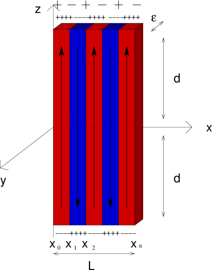
The magnetostatic energy $E_{m}$ can be expressed in terms of the demagnetizing field ${\bf H}_{d}$ as

$$E_{m}=-\frac{1}{2}\,\mu_{0}\int_{sample}\!\!\!\!\!\!\!\!\!{\bf M}\cdot{\bf H}_{d}\,\,dxdydz,$$ (3)

where ${\bf M}$ is the magnetization vector and the integration is taken over the whole sample. Eq. (3) can be rewritten as

$$E_{m}=-\frac{1}{2}\,\mu_{0}\sum_{i=0}^{n-1}(-1)^{i}\int_{x_{i}}^{x_{i+1}}\!\!\!dx\int_{0}^{\epsilon}dy\int_{-d}^{d}dz\,M_{s}\left(\hat{z}\cdot{\bf H}_{d}\right),$$

since the magnetization lies on the $z$ axis. Using that ${\bf H}_{d}=-{\overrightarrow{\nabla}}\phi$, where $\phi$ is the scalar potential, it follows that

$$\hat{z}\cdot{\bf H}_{d}=-\frac{\partial}{\partial z}\phi(x,y,z),$$

and therefore

$$E_{m}=\frac{1}{2}\,\mu_{0}\sum_{i=0}^{n-1}(-1)^{i}\int_{x_{i}}^{x_{i+1}}dx\int_{0}^{\epsilon}dy\int_{-d}^{d}dz\,M_{s}\frac{\partial}{\partial z}\phi(x,y,z)$$

$$=\frac{1}{2}\,\mu_{0}M_{s}\sum_{i=0}^{n-1}(-1)^{i}\int_{x_{i}}^{x_{i+1}}dx\int_{0}^{\epsilon}dy\left[\phi(x,y,d)-\phi(x,y,-d)\right].$$

The scalar potential is given by the surface integral

$$\phi(x,y,z)=\int\!dS\,\,\frac{\sigma}{r}$$

$$=\sum_{j=0}^{n-1}(-1)^{j}\int_{x_{j}}^{x_{j+1}}\!\!\!dx^{\prime}\int_{0}^{\epsilon}\!dy^{\prime}M_{s}$$

$$\times\left[\frac{1}{\sqrt{(x-x^{\prime})^{2}+(y-y^{\prime})^{2}+(z-d)^{2}}}\right.$$

$$\left.-\frac{1}{\sqrt{(x-x^{\prime})^{2}+(y-y^{\prime})^{2}+(z+d)^{2}}}\right],$$

since the surface charge density $\sigma$ value is $M_{s}$ or $-M_{s}$ on the upper and lower interfaces $(x,y,\pm d)$ and $0$ elsewhere. The magnetization is uniform inside the domains, thus no volume density of charge is taken into account.

Thus we obtain

$$E_{m}=\mu_{0}M_{s}^{2}\sum_{i,j=0}^{n-1}(-1)^{i+j}\int_{x_{i}}^{x_{i+1}}\!\!\!dx\int_{x_{j}}^{x_{j+1}}\!\!\!dx^{\prime}\int_{0}^{\epsilon}\!\!\!dy\int_{0}^{\epsilon}\!\!\!dy^{\prime}$$

$$\left[\frac{1}{\sqrt{(x-x^{\prime})^{2}+(y-y^{\prime})^{2}}}-\frac{1}{\sqrt{(x-x^{\prime})^{2}+(y-y^{\prime})^{2}+4d^{2}}}\right].$$ (4)

Assuming that $\epsilon<<2d$, as in most of the samples of experimental interest, we can neglect the term $(y-y^{\prime})^{2}$ with respect to $4d^{2}$ in the Eq. 4. Therefore, the result of the integral is given by

$$E_{m}=\mu_{0}M_{s}^{2}\sum_{i,j=0}^{n-1}(-1)^{i+j}\frac{1}{2}$$

$$\left\{\left[g(x_{i+1},x_{j+1})+g(x_{i},x_{j})-g(x_{i+1},x_{j})-g(x_{i},x_{j+1})\right]\right.$$

$$\left.-\epsilon^{2}\left[f(x_{i+1},x_{j+1})+f(x_{i},x_{j})-f(x_{i+1},x_{j})-f(x_{i},x_{j+1})\right]\right\},$$ (5)

where

$$\left\{\begin{array}[]{lc}\displaystyle f(x,y)=f(y,x)=2\sqrt{4d^{2}+(x-y)^{2}}\\ +(x-y)\ln\left(\frac{y-x+\sqrt{4d^{2}+(x-y)^{2}}}{x-y+\sqrt{4d^{2}+(x-y)^{2}}}\right)\\ \\ g(x,y)=g(y,x)=(x-y)\epsilon^{2}\ln\left(\frac{y-x+\sqrt{\epsilon^{2}+(x-y)^{2}}}{x-y+\sqrt{\epsilon^{2}+(x-y)^{2}}}\right)\\ -\frac{2}{3}|x-y|^{3}+(x-y)^{2}\epsilon\ln\left(\frac{\sqrt{(x-y)^{2}+\epsilon^{2}}-\epsilon}{\sqrt{(x-y)^{2}+\epsilon^{2}}+\epsilon}\right)\\ +\frac{2}{3}\left((x-y)^{2}+\epsilon^{2}\right)^{3/2}\end{array}\right.$$

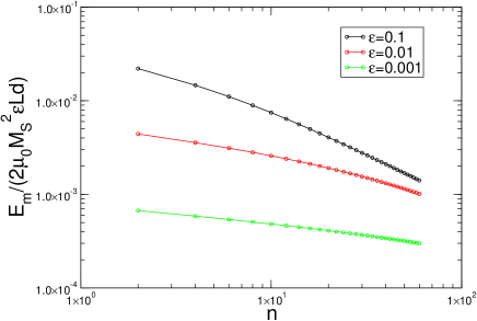
To give an idea of the behavior of the magnetostatic energy, in Fig. (2) we have plotted $E_{m}(t)$ for a sample of fixed length $L$ and $d$ and for three values of the thickness, $\epsilon=0.1;0.01;0.001$, as a function of the number of (periodic) domains. As it can be seen, from a purely magnetostatic point of view, the energy is a decreasing function of the number of domains. In fact, the total number of domains in a sample is determined by the interplay of the magnetostatic term and the domain wall energy, linearly increasing as a function of $n$  bertotti .

Figure 2: (Color online) Magnetostatic energy $E_{m}$ as a function of the number of domains $n$, for three different values of the system thickness $\epsilon=0.1;0.01;0.001$, and for $L=1.$, and $d=10$, calculated for even numbers of domains. Solid lines are guides to the eye.

The magnetostatic force on the $k$-th wall at time $t$ is thus

$$F_{m}(k,t)=-\frac{\partial E_{m}}{\partial x_{k}(t)}$$

$$=2\mu_{0}M_{s}^{2}\sum_{i=0}^{n-1}(-1)^{i+k}\left[\frac{\partial g(x_{i+1},x_{k})}{\partial x_{k}}-\frac{\partial g(x_{i},x_{k})}{\partial x_{k}}\right.$$

$$\left.-\epsilon^{2}\left(\frac{\partial f(x_{i+1},x_{k})}{\partial x_{k}}-\frac{\partial f(x_{i},x_{k})}{\partial x_{k}}\right)\right],$$ (6)

where

$$\frac{\partial f(x,y)}{\partial y}=-\frac{\partial f(x,y)}{\partial x}=\ln\left(\frac{y-x+\sqrt{4d^{2}+(x-y)^{2}}}{x-y+\sqrt{4d^{2}+(x-y)^{2}}}\right)$$

$$\frac{\partial g(x,y)}{\partial y}=-\frac{\partial g(x,y)}{\partial x}=2(x-y)\sqrt{\epsilon^{2}+(x-y)^{2}}$$

$$+2\epsilon(x-y)\ln\left(\frac{\sqrt{\epsilon^{2}+(x-y)^{2}}-\epsilon}{\sqrt{\epsilon^{2}+(x-y)^{2}}+\epsilon}\right)$$

$$+\epsilon^{2}\ln\left(\frac{y-x+\sqrt{\epsilon^{2}+(x-y)^{2}}}{x-y+\sqrt{\epsilon^{2}+(x-y)^{2}}}\right)-2(x-y)^{2}sign(x-y).$$ (7)

Figure 3: (Color online) Magnetostatic force $F_{m}(k,t)$ on the $k$-th domain wall as a function of $k$ (red dots), for a periodic configuration of the domain walls positions. The sample has $n=21$ domains, $\epsilon=0.002$, $d=10$, and $L=1$. The solid line is a guide to the eye.

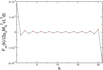
In Fig. (3) we show the magnetostatic force $F_{m}(k,t)$ calculated at each wall $k$ for a periodic configuration of $n=21$ domains. As it could be seen, walls with $k$ of opposite parities are driven in opposite directions, and the absolute value of $F_{m}(k,t)$ is higher for the external walls, which is a finite size effect tending to reduce the size of the boundary domains. For a large odd number of domains, in the center of the sample, all the $F_{m}(k,t)$ would be equal in magnitude, as it can be seen in Fig. (3). For an even number of domains, the central wall experiences a zero force for symmetry reasons. As expected, for a generic (even or odd) number of domains, the effect of the magnetostatic force is to move the walls in the direction that decreases the magnetization, in order to minimize the magnetostatic energy [see Eq. (3)].

II.2 Disorder

Different sources of inhomogeneities are found in virtually all ferromagnetic materials. The presence of structural disorder is essential to understand the hysteretic behavior, and especially to account for the residual coercive field when the frequency of the external driving field vanishes. Disorder is provided by vacancies, non-magnetic impurities, dislocations or grain boundaries in crystalline systems, variations of the easy axis between different grains for polycrystalline materials, and internal stresses for amorphous alloys.

We consider here only quenched (frozen) disorder that does not evolve on the timescale of the magnetization reversal, which is usually a realistic approximation for ferromagnetic systems. At the beginning of a simulation, we extract the positions of a fixed number $n_{p}$ of pinning centers with a uniform probability distribution all over the sample. Each pinning center interacts with every domain wall by a located potential of the type

$$U_{p}(x)=A\exp[-(x/\xi)^{2}],$$ (8)

where $x$ is the distance between the pinning center and the wall, $\xi$ is a correlation length and the amplitude $A$ is extracted from a uniform distribution, considering that the strength of the pinning centers should vary for structural reasons. In this way we produce a disordered landscape in which the domain walls evolve.

II.3 External field

The interaction between a ferromagnetic system and an external magnetic field ${\bf H}$ is described by the energy term:

$$E_{ext}=-\mu_{0}\int_{sample}{\bf M}\cdot{\bf H}\,dV.$$ (9)

In our model the uniaxial anisotropy and the external time dependent magnetic field $H_{ext}(t)$ are parallel to the easy axis of the sample, and thus parallel or anti-parallel to the magnetization. Thus in this case the total energy is

$$E_{ext}=2d\epsilon\mu_{0}M_{s}H_{ext}\sum_{i=0}^{n-1}(-1)^{i}\left(x_{i+1}(t)-x_{i}(t)\right),$$

and the external field contribution $F_{ext}(k,t)$ to the force $F(k,t)$ on the $k$-th wall at time $t$ is given by the partial derivative of Eq. (9) with respect to the wall position $x_{k}(t)$, and could be thus written as

$$F_{ext}(k,t)=4\mu_{0}M_{s}d\epsilon H_{ext}(t)(-1)^{k+1},$$ (10)

which depends of course on the parity of the domain wall.

III Demagnetizing factor and magnetostatic susceptivity

An interesting analytical result that could be obtained from our model is the dependence of the demagnetizing factor $\kappa$ on the number $n$ of the parallel domain walls. The parameter $\kappa$ enters as a mean field term in several domain wall models used to describe the BN ABBM ; zapperi ; zapperi2 ; urbach ; bahiana . Its precise dependence on the sample geometry is usually approximated considering a uniformly magnetized sample and the domain structure is ignored. Understanding this point is important since $\kappa$ determines for instance the size dependence of the Barkhausen avalanche distribution dz .

The demagnetizing factor $\kappa$ can be rigorously defined for uniformly magnetized ellipsoid from the relation $H_{d}=-\kappa M$. In more general situations, we can define it as an effective quantity linking the average demagnetizing field to the magnetization $\kappa\equiv-\langle H_{d}\rangle/M$. Here we compute $\kappa$ from the magnetic response of the system to a small perturbative external field. Since at equilibrium a small change in the external field is compensated by an increase in the demagnetizing field ($H_{d}+H_{ext}=0$), we can link $\kappa$ to the magnetostatic susceptivity $\chi=dM/dH_{ext}$ by the relation $\kappa=1/\chi$.

For an extended system with a large and even number of domains $n$, the equilibrium configuration consists of a domain wall array

$$x_{i}=\frac{iL}{n}\,\,\,\,\,\,\,\,\,\forall i$$

(note: in what follows we will omit the $t$ dependence of the functions). We can choose a positive perturbative field $\delta H_{ext}$ and thus consider the perturbed walls positions:

$$\left\{\begin{array}[]{l}\displaystyle x_{i}=\frac{iL}{n}+(-1)^{i+1}u\\ \\ x_{0}=0\\ \\ x_{n}=L\end{array}\right.$$

that correspond to a (small) increase of the magnetization $dM\sim nu$, with $u>0$, uniformly distributed over the domain walls. Since the calculation of the magnetic susceptivity is quite involved, we discuss it in the Appendix and report here only the final result:

$$\chi=\frac{\partial M}{\partial H_{ext}}=\frac{1}{\kappa}=\frac{d}{\epsilon A(n)},$$ (11)

where

$$A(n)=2\left[\gamma+\ln(n)\right],$$

and $\gamma\simeq 0.577215$. Higher order corrections in $n$ have been neglected.

In Fig. 4 we compare the results of our simulations and the theoretical result of Eq. 11, for a system with $d=400$, $\epsilon=0.01$ and $L=1$, without disorder, by studying $\kappa$ as a function of the number of domain walls $n$ (coinciding with the number of domains in the limit $n\rightarrow\infty$). The simulations are performed starting from a periodic configuration of a high and even number of domains, and letting the walls relax under an external field that is very low, in order to have a displacement from the equilibrium position of the walls of the order of some per cents of the distance between nearest-neighbor walls. To fulfill the hypothesis under which Eq. 11 is calculated, we use here periodic boundary conditions. As it can be seen, the agreement between theory and simulations is excellent, even if the simulations have been performed for finite samples. The value of the magnetic susceptivity is of the order $1/\kappa=\chi\simeq 10^{4}$, which is a realistic value for a ferromagnetic system. It would be very interesting to test the prediction of Eq. 11 with experimental results on materials with low disorder. Finally, it is interesting to notice that the demagnetizing factor $\kappa=1/\chi$ displays an inverse dependence on the sample length $d$ and a linear dependence on the thickness $\epsilon$. Hence, as expected, reducing the sample aspect ratio leads to an increase in $\kappa$. This fact has been exploited in Ref. dz, to tune $\kappa$ and study its effect on the BN.

Figure 4: Demagnetizing factor $\kappa$ as a function of the number of domain walls $n$ (semilogarithmic scale): comparison between simulation results and perturbative calculation (dashed line) for $d=400$, $\epsilon=0.01$, and for unitary $L$.

IV Numerical model

In the previous sections we have calculated the various contributions to the total force acting on each wall (Eq. 1) thus it is now possible to simulate the dynamics of the system. Since the number of the walls is $n$, and we consider in this part closed boundary conditions (the boundary walls do not move), we have to write down $n-2$ equations of motion given by

$$\Gamma\frac{dx_{k}}{dt}=F(k,t)=F_{m}(k,t)+F_{ext}(k,t)+F_{dis}(k,t).$$ (12)

In the following we set the damping coefficient $\Gamma$ to unity. We integrate these equations using a fourth order Runge-Kutta algorithm. The external magnetic field is a saw-tooth signal with rate $\omega$, being $\dot{H}\propto\omega$.

We always start our simulations with an $M=0$ at $H_{ext}=0$ periodical configuration, and drive the sample to positive and then to negative saturation. We include the possibility of nucleation and annihilation of the domain walls by fixing a minimum interaction range between two nearest-neighbor walls, namely $\delta_{min}$. If two walls get closer than $\delta_{min}$, we stop them and consider the pair of walls as annihilated. This means that their contribution on the sum involved in the calculation of long-range magnetostatic force (see Eq. 6), and thus their effect on the equations of motion of the other walls, is no more considered. Besides, we go on calculating the total force on the annihilated pair of walls. When this force become strong enough (and of the correct sign) to let them escape from the range $\delta_{min}$, we nucleate them and consider again their contribution to the magnetostatic force calculation, Eq. 6. This corresponds to have a nucleation barrier equal to zero. Since we are interested in the study of Barkhausen noise and of the coercive field behavior connected to dynamic hysteresis, this choice does not influence our results, as we have checked. In fact, all the phenomena that we are interested in take place in the central region of the hysteresis loop, namely the one close to the coercive field $H_{c}$, while the choice of the nucleation barrier involves only the region of the cycle close to saturation. Moreover, for the same reason, our results are independent on the choice of $\delta_{min}$, as long as it is chosen in a reasonable range.

V Coercive field and dynamic hysteresis

V.1 Dynamic hysteresis

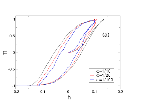
We first consider the effect of the external field rate on the hysteretic behavior. In Fig. 5(a) we show the hysteresis loops obtained for various rates for a system with $n=20$ domains (since from now we will deal with a reasonably high number of domains, we will use with a slight abuse of terms $n$ for the number of domains), where $m$ is the normalized magnetization $m=M/M_{s}$ and $h$ is the normalized magnetic field $h=H/M_{s}$. As expected from experiments and general considerations, small (high) frequencies correspond to narrow (large) cycles. To quantify this observation we can focus on the coercive field $H_{c}$ behavior. In Fig. 5(b) we show the dependence of $H_{c}$ on the field rate $\omega$.

Figure 5: (Color online) (a) Hysteresis loops for different external field rates, for a system with $n=20$ domains, and (b) Coercive field as a function of the external field rate for three different system sizes, $n=20,40,60$; $h_{c}$ vs $dh/dt$ in a linear plot, in comparison with a square root fit (dashed line) and the fit with the power loss formula (continuous line, see text). Every point is mediated over $100$ realizations corresponding to different disorder configurations.

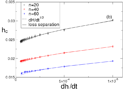For all the considered values of $n$ in Fig. 5, $n=20,40,60$ (for a discussion of the behavior of $H_{c}$ as a function of the number of domains $n$ see the next subsection), $H_{c}$ shows an increasing dependence on $\omega$. The $H_{c}$ dependence on $\omega$ is quite close to a power law of the form

$$H_{c}=H_{p}+A\omega^{1/2},$$ (13)

as suggested for experiments on permalloy thin films and microstructures fabricated from the same sample nistor , and by the theory presented in Ref. lyuksyutov, .

Nevertheless, as it can be seen in Fig.5(b), our curves are best fitted by the loss separation formula bertotti ; colaiori ,

$$H_{c}=H_{p}+C_{ex}[(1+r\dot{H})^{1/2}-1],$$ (14)

where $C_{ex}=n_{0}V_{0}/2$, and $r=4\Gamma\mu/(n_{0}^{2}V_{0})$. Here $n_{0}$ is the number of active walls in the quasi-static limit ($\omega\rightarrow 0$), $V_{0}$ is a characteristic field which controls the increase of $n_{0}$ due to the excess field, $\mu$ is the permeability and $H_{p}$ is the static (hysteretic) component. The fit parameters values are shown in table 1.

n	20	40	60
$H_{p}$	0.024	0.019	0.016
$C_{ex}$	0.003	0.003	0.0036
r	6622	4752	2989
$\mu$	183	153	173
$n_{0}$	18	21	32
$V_{0}$	0.0003	0.0003	0.0002

Table 1: Fit parameter values for Fig. 5(b).

The behavior of $H_{c}$ as a function of $\omega$, suggested in Eq. 14, means that in the adiabatic limit (low frequencies) $H_{c}$ goes to a non-vanishing value $H_{p}$ that we can interpret as the pinning dominated quasi-static component due to structural disorder, while the behavior of $H_{c}$ in the high rate regime represents the domain wall dominated dynamic contribution. Moreover, the scaling function of Eq. 14 describes the evolution from the adiabatic to the domain wall dominated power-law behavior without invoking mechanism crossover between domain wall propagation and nucleation of new domains. In fact, even if the nucleation process is included in our model, besides in a very simplified form, nucleation takes place only in the regions of the hysteresis loops very close to saturation. Thus the cycles are very oblique [see Fig. 5(a)]. Such a kind of hysteresis loops are expected to be dominated by domain wall motion.

V.2 Role of the number of domains

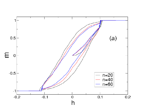
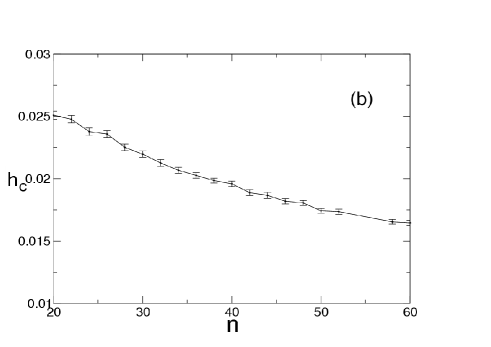
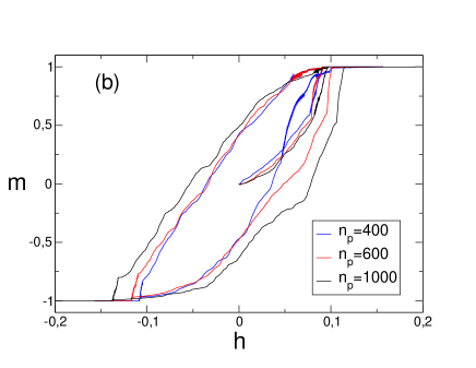
Another interesting issue to analyze is the effect of the number of domains $n$ on the system behavior. We remind here that at the beginning of each simulation we set the maximum number of domains of the specimen. This number can decrease down to one while driving the system to saturation, and then, increasing the external field, it is completely restored around the coercive field. From a qualitative point of view, keeping constant the other system parameters (i.e. the physical dimensions of the specimen under study and the pinning centers density and strength $f_{0}$), a high (low) number of domains corresponds to hysteresis loops with a lower (higher) permeability, in accord with Eq.11, as it can be seen in Fig. 6(a). This happens because the increase of the domain number increases the relative relevance, in the total force balance, of the dipolar contribution. In fact, an absence of collective behavior leads to square shaped cycles, where the whole magnetization reversal process takes place in a few avalanches. Otherwise, in materials in which dipolar interactions are relevant, oblique hysteresis loops are expected. In our simulations, the coercive field $H_{c}$ decreases as a function of $n$, as expected [see Fig. 6(b)].

Figure 6: (Color online) (a) Some hysteresis loops for different system sizes, $n=20,40,60$, for an applied field rate $\omega=1/20$, and (b) Coercive field $H_{c}$ as a function of the number of domains $n$. Every point is an average on $100$ samples, corresponding to different disorder realization, for an applied field rate $\omega=1/1000$. The line is a guide to the eye.

V.3 Effect of disorder

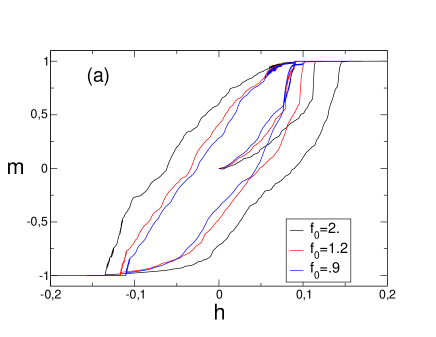
As we have already mentioned, the presence of structural disorder has a crucial role in the physics of ferromagnetic systems. Disorder pins the domain walls, that thus are not able to move until the external field reaches a sufficient value to overcome the pinning and let the wall move again. Hence we will expect, from this simple argument, that more disordered systems have larger hysteresis loops compared to purer specimens, for the same $\omega$.

Figure 7: (Color online) hysteresis loops for varying: (a) disorder strength $f_{0}$ ($n_{p}=600$) and (b) number of pinning centers $n_{p}$ ($f_{0}=1.2$). The rate is $\omega=1/50$.

We remind here that it is difficult to quantify the disorder contribution in real systems. In our model we have two degrees of freedom to control the disorder: we can tune the density of pinning centers (by controlling the total number of pinning sites $n_{p}$) and their strength $f_{0}$.

In Fig. 7 we show some hysteresis cycles for varying values of the two parameters $f_{0}$ [see panel (a)] and $n_{p}$ [see panel (b)]. As we can see, their effect on the loops is qualitatively similar, and the behavior for increasing disorder (i.e. larger cycles for larger disorder) is in agreement with the general argument explained above.

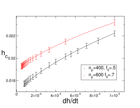
In Fig. 8, we show the coercive field behavior for increasing disorder, intended here as increasing both the values of $n_{p}$ and $f_{0}$: as expected, stronger disorder implies higher coercive field. Moreover, it is important to notice that even varying the disorder strength or density, the $H_{c}$ dependence on the square root of the applied field rate does not change.

Figure 8: (Color online) The reduced coercive field $h_{c}$ dependence on the external field rate $dh/dt$ for a system with $n=40$ domains and two different number of pinning centers $n_{p}$ and disorder amplitude $f_{0}$. The applied field rate is $\omega=1/1000$. Data are fitted by Eq.14. Fit parameters are $H_{p}=0.019$, $C_{ex}=0.003$ and $r=4752$ for $n_{p}=400$; $H_{p}=0.017$, $C_{ex}=0.0038$ and $r=4752$ for $n_{p}=600$.

VI Barkhausen noise

The Barkhausen noise is an unavoidable feature of magnetic hysteresis in disordered samples and its statistical properties have been widely studied in experiments and models dz . The experiments in soft ferromagnetic materials have been divided into universality classes depending on the avalanche distributions dz . Experimental results are well described by models involving a single flexible domain wall, and ignoring any interactions between different walls. Different universality classes are set by the dominant interactions between parts of the walls. Here we explicitely ignore these local interactions and want to account only for the interactions between walls.

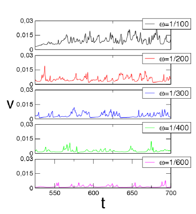
In Fig. 9 we show some simulated signals for various rates of the external field. Partial regions are chosen for the signals, corresponding to the same time interval. As it can be seen, our results reproduce a well-known characteristic of the experimental Barkhausen noise: at low frequencies, the signal is composed of separated avalanches, while this property is progressively lost at higher frequencies. In the latter case, the signal appears as a continuous sequence of peaks and the single avalanches are no more distinguishable. We have analyzed the Barkhausen signal considering the distribution of the signal amplitude, avalanche sizes and durations.

Figure 9: (Color online) Time sequences of Barkhausen noise. The labels indicate the applied field rate. We report portions of simulated signals corresponding to the same time interval. The time is measured considering an integrating time step $\Delta t=0.05$.

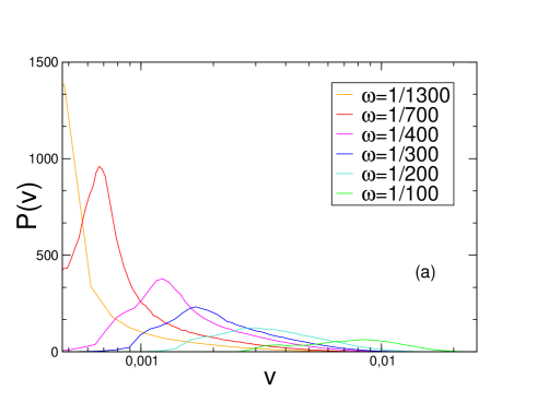
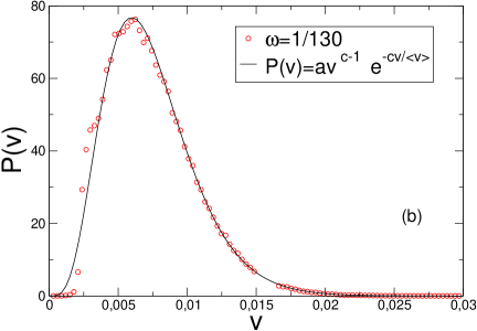
The amplitude probability distribution of the magnetic induction flux rate $\dot{\phi}$ is a measurable quantity and thus has been often used in order to test the reliability of a model for Barkhausen noise (see for instance Ref. ABBM, ). In fact, the flux rate is related to the velocity of the domain walls $v$. In Fig. 10(a) we show the rate dependence of the probability amplitude distribution. In the non-adiabatic limit, in fact, the domain walls velocity is expected to depend on $\omega$. We notice that $P(v)$ passes from a almost symmetric shape for very high frequencies to an asymmetric one for low frequencies.

In the ABBM model ABBM , the predicted shape of the amplitude probability distribution is a Gamma function

$$P(v)\propto v^{c-1}e^{-cv/\langle\!v\!\rangle}.$$ (15)

We remind here that this formula is obtained under the assumption that the disorder is a correlated (Brownian) process.

The mechanism giving rise to the Barkhausen effect is the domain walls motion, and that a domain wall motion can be described as a stationary Markov process, associated with fixed and well-defined values of the magnetization rate imposed to the system and of the permeability of the specimen $\mu$, associated with the part of the hysteresis loop where the domain wall motion is assumed to take place. Even if our model is different from the single wall model ABBM, the formula of Eq. 15 is able to fit our probability distributions $P(v)$ for high rates, although it does not supply a suitable explanation for the low rate regime [see Fig. 10(b)].

Figure 10: (Color online) (a) Probability distribution of the signal amplitude (i.e. of the domain walls velocity) $v$, for various frequencies $\omega$ of the external magnetic field ($\omega=1/1300,1/700,1/400,1/300,1/200,1/100$, for a system with $n=60$ domains. (b) Probability distribution of the signal amplitude for $n=60$ and $\omega=1/130$, fitted with the ABBM function, $P(v)=av^{c-1}exp(-cv/<\!v\!>)$.

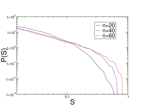
Next, we evaluate the probability distribution for the duration $T$ and the size $S\equiv\int^{T}dtv(t)$ of the avalanches. The distributions are shown in Figs. 11(a) and 11(b).

Figure 11: (Color online) (a) Probability distribution of the avalanche size $S$, and (b) Probability distribution of the avalanche duration $T$, for three different system sizes ($n=20,40,60$).

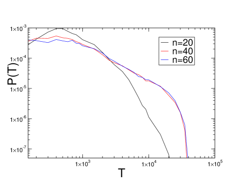As it can be seen, both distributions display a power law behavior of the type $P(S)\sim S^{-\tau}$ and $P(T)\sim T^{-\alpha}$, for almost two decades for the maximum studied size ($n=60$), with a cutoff. The scaling exponents of these distributions are respectively $\tau\sim 1.1$ and $\alpha\sim 1.2$. These exponent values, however, have never been reported for bulk soft magnetic materials where parallel domain walls are commonly observed dz . This is not surprising as we neglect local interactions, and any deformation of the domain wall. It is nevertheless remarkable that just the combined effect of dipolar interactions and disorder yields power law avalanche distribution in a multi-domain model. The latter appear, however, essential to recover quantitatively the experimental results in bulk samples dz . To completely resolve this issue, it would be necessary to study the dynamics of an array of flexible and interacting domain walls.

VII Conclusions

The technological and theoretical relevance of the hysteresis in ferromagnetic systems motivates the effort in modeling the phenomenon. Of particular interest is the study of the dynamic hysteresis, connected with the power losses of the material, and of the Barkhausen noise, which represents a tool for the investigation of the magnetization dynamics.

In this article we have presented a model for the dynamics of a system of parallel and rigid uncharged (Bloch) domain walls, moving in a disordered landscape driven by an external magnetic field. The analyzed configuration of domain walls is a common case both in two and three dimensional samples. Our model is based on the interplay between the long-ranged dipolar interactions and the external field and disorder contributions. Due to the simplicity of the wall configuration, we calculated perturbatively the demagnetizing factor and the magnetostatic susceptibility as functions of the geometrical parameters of the system, namely the thickness, the height and the number of domains at equilibrium, in the absence of external magnetic field. The simulation results perfectly agree with the calculations, and we have thus been able to link a measurable macroscopic quantity to the microscopical system behavior. Next, we have investigated the dynamic hysteresis by means of the study of the coercive field behavior, obtained by simulating the equations of motion of the walls array. The coercive field displays a power law behavior as a function of the applied field rate, with an exponent in agreement with experimental available data. Finally we have analyzed the Barkhausen noise, constructing the probability distributions of the Barkhausen avalanches size and time duration, and found power laws with cutoffs for both the distributions. Moreover we find that the probability distribution of domain walls velocity deviates at low driving rates from the ABBM related formula. Since the latter model is based on the motion of a single domain wall, we can conclude that the multi-domain effects are important in ferromagnetic systems, since they affect system parameters like the demagnetizing factor and the behavior of the Barkhausen noise.

VIII appendix

We can develop the magnetostatic force $F_{m}(k)$ on a generic wall $k$ (see Eq. 6), around its equilibrium position:

$$F_{m}(k)=F_{m}^{eq}(k)+\delta F_{m}(k)=\delta F_{m}(k),$$

since the equilibrium term $F_{m}^{eq}(k)$ is $0$ by definition. It follows:

$$F_{m}(k)=\sum_{j=0}^{n}\left.\frac{\partial F_{m}(k)}{\partial x_{j}}\right|_{u_{j}=0}(-1)^{j+1}u_{j}$$

$$=\sum_{j=1}^{n-1}\left.\frac{\partial F_{m}(k)}{\partial x_{j}}\right|_{u_{j}=0}(-1)^{j+1}u_{j},$$ (16)

where the last equality descends from the fact that the boundaries of the sample are fixed.

For simplicity in the calculations, let us separate the contribution $k=j$ from the others, and rewrite Eq. 16 as:

$$F_{m}(k)=\frac{\partial F_{m}(k)}{\partial x_{k}}u_{k}(-1)^{k+1}+\sum_{j\neq k}\left.\frac{\partial F_{m}(k)}{\partial x_{j}}\right|_{u_{j}=0}(-1)^{j+1}u_{j}$$

$$=2M_{s}^{2}\mu_{0}(-1)^{k+1}u_{k}\sum_{j=1}^{n-1}\left[\left(\frac{\partial^{2}g(x_{j+1},x_{k})}{\partial x_{k}^{2}}-\epsilon^{2}\frac{\partial^{2}g(x_{j},x_{k})}{\partial x_{k}^{2}}\right)\right.$$

$$\left.-\epsilon^{2}\left(\frac{\partial^{2}f(x_{j+1},x_{k})}{\partial x_{k}^{2}}-\epsilon^{2}\frac{\partial^{2}f(x_{j},x_{k})}{\partial x_{k}^{2}}\right)\right]$$

$$+4M_{s}^{2}\sum_{j=0}^{n-1}(-1)^{j+k}\left(\frac{\partial^{2}g(x_{j},x_{k})}{\partial x_{k}^{2}}-\epsilon^{2}\frac{\partial^{2}f(x_{j},x_{k})}{\partial x_{k}^{2}}\right)u_{j}(-1)^{j+1},$$

where we have used the symmetry properties of the derivatives (see Eq. 7 ). In the last sum we have included again the $k$-th term since it is null. If we neglect the contribution from the boundaries, that could be done since we are in the $n\rightarrow\infty$ case, we can translate $j+1\rightarrow j$ in the first sum, together with the sum index. We obtain:

$$F_{m}(k)=4\mu_{0}M_{s}^{2}u_{k}\sum_{j}(-1)^{j}\left(\frac{\partial^{2}g(x_{j},x_{k})}{\partial x_{k}^{2}}-\epsilon^{2}\frac{\partial^{2}f(x_{j},x_{k})}{\partial x_{k}^{2}}\right)$$

$$-4\mu_{0}M_{s}(-1)^{k}\sum_{j}(-1)^{j}u_{j}\left(\frac{\partial^{2}g(x_{j},x_{k})}{\partial x_{k}^{2}}-\epsilon^{2}\frac{\partial^{2}f(x_{j},x_{k})}{\partial x_{k}^{2}}\right).$$

So finally, it results

$$F_{m}(k)=4\mu_{0}M_{s}^{2}\sum_{j=0}^{n-1}\left(\frac{\partial^{2}g(x_{j},x_{k})}{\partial x_{k}^{2}}-\epsilon^{2}\frac{\partial^{2}f(x_{j},x_{k})}{\partial x_{k}^{2}}\right)$$

$$\times\left((-1)^{j}u_{k}-(-1)^{k}u_{j}\right),$$ (17)

where the double derivatives of Eq. 7 are:

$$\left\{\begin{array}[]{l}\displaystyle\frac{\partial^{2}f(x,y)}{\partial x^{2}}=-\frac{2}{\sqrt{4d^{2}+(x-y)^{2}}}\\ \\ \displaystyle\frac{\partial^{2}g(x,y)}{\partial x^{2}}=4\left(\sqrt{\epsilon^{2}+(x-y)^{2}-|x-y|}\right)\\ \\ \displaystyle+2\epsilon\ln\left(\frac{\sqrt{\epsilon^{2}+(x-y)^{2}}-\epsilon}{\sqrt{\epsilon^{2}+(x-y)^{2}}+\epsilon}\right)\end{array}\right.$$ (18)

In order to handle analytically Eq. 17, let us restrict our study to the limit $\epsilon<<|x-y|<<L<<d$, which is the physical case in most ferromagnetic samples. The second derivatives of Eq. 18 thus become

$$\left\{\begin{array}[]{l}\displaystyle\frac{\partial^{2}f(x,y)}{\partial x^{2}}=-\frac{1}{d}\\ \\ \displaystyle\frac{\partial^{2}g(x,y)}{\partial x^{2}}=-\frac{2\epsilon^{2}}{|x-y|}\end{array}\right.$$ (19)

and $F_{m}(k)$ could be in this limit rewritten:

$$F_{m}(k)=4\mu_{0}M_{s}^{2}\sum_{j}\left(-\frac{2\epsilon^{2}}{|x_{j}-x_{k}|}+\frac{\epsilon^{2}}{d}\right)$$

$$\times(-1)^{j+k}\left((-1)^{k}u_{k}-(-1)^{j}u_{j}\right).$$ (20)

To have some insight on Eq. 20, we can study the effect of the magnetostatic force in two simplified situations:

• Let us imagine that all the walls are fixed but the $k$-th. Thus Eq. 20 can be rewritten:

  $$F_{m}(k)=-8\mu_{0}M_{s}^{2}\epsilon^{2}\sum_{i}\frac{(-1)^{i+k}}{|x_{i}-x_{k}|}(-1)^{k}u_{k}$$

  $$=-8\mu_{0}M_{s}^{2}\epsilon^{2}u_{k}\sum_{i}\frac{(-1)^{i}}{|x_{i}-x_{k}|},$$

  that means that every wall $i$ contributes with a term of sign $(-1)^{i+1}$. Since the most important contribution in the sum of Eq. 20 is due to the nearest neighbors, if $k$ is odd (even) and has thus a positive (negative) perturbation on the position, it will be subject to a negative (positive) magnetostatic force, recalling the wall to the equilibrium position.

• Considering the case with all the perturbations $u_{i}=u$, $\forall i$. The magnetostatic force becomes

  $$F_{m}(k)=4M_{s}^{2}\epsilon^{2}u\sum_{i}\left(-\frac{2}{|x_{i}-x_{k}|}+\frac{1}{d}\right)$$

  $$\times(-1)^{i+k}\left((-1)^{k}-(-1)^{i}\right).$$ (21)

  So only the walls with the opposite parity with respect to $k$ will contribute to $F_{m}(k)$. Thus the even (odd) walls, that have a negative (positive) displacement, will experience a positive (negative) force, recalling the wall to the equilibrium position.

Let us restrict ourselves in the following to the limit above, $u_{i}=u$, $\forall i$. So, starting from Eq. 21, we can write

$$F_{m}(k)=\frac{4\mu_{0}M_{s}^{2}\epsilon^{2}u}{d}\sum_{i}\left((-1)^{i}-(-1)^{k}\right)$$

$$-\frac{8\mu_{0}M_{s}^{2}\epsilon^{2}un}{L}\sum_{i}\frac{1}{|i-k|}\left((-1)^{i}-(-1)^{k}\right),$$

using the definition $x_{i}=iL/n$. Since $L<<d$ and $n/|i-k|\geq 1$ $\forall$ $i,k$, we can approximate

$$F_{m}(k)\simeq-\frac{8\mu_{0}M_{s}^{2}\epsilon^{2}un}{L}\sum_{i}\frac{1}{|i-k|}\left((-1)^{i}-(-1)^{k}\right)$$

$$=\alpha\sum_{i}\frac{1}{|i-k|}\left((-1)^{i}-(-1)^{k}\right),$$

defining $\alpha=8\mu_{0}M_{s}^{2}\epsilon^{2}un/L$. In the sum

$$F_{m}(k)=\alpha(-1)^{k}\sum_{i}\frac{1}{|i-k|}\left((-1)^{i+k}-1\right),$$

the only non null terms are the $i$th terms $i^{\prime}$ with opposite parity with respect to $k$, that lead to a contribution

$$F_{m}(k)=\alpha(-1)^{k}(-2)\sum_{i^{\prime}=0}^{n}\frac{1}{|i-k|}.$$

Since $n\rightarrow\infty$, we could consider $k$ in the middle of the sample and write

$$F_{m}(k)=-4\alpha(-1)^{k}\sum_{i^{\prime}=1}^{n/2}\frac{1}{i}=-4\alpha(-1)^{k}\sum_{i=1}^{n/4}\frac{1}{2i-1}$$

$$=-2\alpha(-1)^{k}\left[\gamma+\ln\left(\frac{n}{4}\right)+2\ln{(2)}\right],$$

by using the sum of an harmonic finite series of odd terms, where $\gamma=0.577215$. So finally

$$F_{m}(k)=\frac{8\mu_{0}M_{s}^{2}\epsilon^{2}un}{L}(-1)^{k}A(n)$$

where

$$A(n)=2\left[\gamma+\ln\left(\frac{n}{4}\right)+2\ln{(2)}\right]=2\left[\gamma+\ln(n)\right].$$

The energy term due to the external magnetic field is given by Eq. 9, and in this case could be written

$$E_{ext}=-4\mu_{0}M_{s}H_{ext}d\epsilon\sum_{i}u_{i}.$$

Therefore, $F_{ext}(k)$ is given by:

$$F_{ext}(k)=-\frac{\partial E_{ext}}{\partial x_{k}}=\frac{4\mu_{0}M_{s}H_{ext}d\epsilon\sum_{i}u_{i}}{(-1)^{k+1}u_{k}}$$

$$=(-1)^{k+1}4\mu_{0}M_{s}H_{ext}d\epsilon.$$

Since at the equilibrium the total force $F=0$, in absence of disorder it must be

$$F_{m}(k)+F_{ext}(k)=0$$

$$=\frac{8\mu_{0}M_{s}^{2}\epsilon^{2}un}{L}(-1)^{k}A(n)+(-1)^{k+1}4\mu_{0}M_{s}H_{ext}d\epsilon,$$

from which follows

$$H_{ext}=\frac{2\epsilon uA(n)M_{s}n}{Ld}.$$

The magnetization $M$ could be written

$$M=\frac{4ud\epsilon M_{s}n}{2dL\epsilon}=\frac{2uM_{s}n}{L}.$$

So finally we can calculate the magnetic susceptivity $\chi$:

$$\chi=\frac{\partial M}{\partial H_{ext}}=\frac{M}{H_{ext}}=\frac{d}{\epsilon A(n)},$$ (22)

which was our goal.

References

- (1) G. Bertotti, Hysteresis in magnetism (Academic Press, San Diego, 1998)
- (2) J. P. Sethna, K. Dahmen, S. Kartha, J. A. Krumhansl, B. W. Roberts and J. D. Shore, Phys. Rev. Lett. 70, 3347 (1993)
- (3) J. P. Sethna, K. A. Dahmen and C. R. Myers, Nature, 410 242 (2001)
- (4) E. Vives and A. Planes, Phys. Rev. B 50 3839 (1994)
- (5) E. Vives and A. Planes, J. Mag. Magn. Mat. 221 164 (2000)
- (6) E. Vives and A. Planes, Phys. Rev. B 63 134431 (2001)
- (7) B. K. Chakrabarti and M. Acharyya, Rev. Mod. Phys. 71, 847 (1999)
- (8) M. Acharyya and B. K. Chakrabarti, Phys. Rev. B 52, 6550 (1995)
- (9) S. W. Sides, P. A. Rikvold and M. A. Novotny, Phys. Rev. E 59,2710 (1999)
- (10) H. L. Richards, M. A. Novotny and P. A. Rikvold, Phys. Rev B 54, 4113 (1996)
- (11) S. W. Sides, P. A. Rikvold and M. A. Novotny, Phys. Rev. E 57, 6512 (1998)
- (12) I. F. Lyuksyutov, T. Nattermann and V. Pokrovsky, Phys. Rev. B 59, 4260 (1999)
- (13) B. Alessandro, C. Beatrice, G. Bertotti and A. Montorsi, J. Appl. Phys. 68 2901 (1990)
- (14) S. Zapperi, P. Cizeau, G. Durin and H. E. Stanley, Phys. Rev. B 58, 6353 (1998)
- (15) P. Cizeau, S. Zapperi, G. Durin and H. E. Stanley, Phys. Rev. Lett. 79 4669 (1997)
- (16) J. S. Urbach, R. C. Madison, J. T. Markert, Phys. Rev. Lett. 75 276 (1995)
- (17) O. Narayan, Phys. Rev. Lett. 77 3855 (1996)
- (18) M. Bahiana, B. Koiller, S. L. A. de Queiroz, J. C. Denardin and R. L. Sommer, Phys. Rev. E 59 3884 (1999)
- (19) S. L. A. de Queiroz and M. Bahiana, Phys. Rev. E 64 066127 (2001)
- (20) T. A. Moore and J. A. C. Bland, J. Phys.: Condens. Matter 16, R1369 (2004)
- (21) C. Nistor, E. Faraggi, and J. L. Erskine, Phys. Rev. B 72, 014404 (2005)
- (22) B. Raquet, R. Mamy and J. C. Ousset, Phys. Rev. B 54 4128 (1996)
- (23) Y.-L. He and G.-C. Wang, Phys. Rev. Lett. 70 2336 (1993)
- (24) C. N. Luse and A. Zangwill, Phys. Rev. E 50, 224 (1994)
- (25) Q. Jiang, H.-N. Yang and G.-C. Wang, Phys. Rev. B 52 14911 (1995)
- (26) J.-S. Suen and J. L. Erskine, Phys. Rev. Lett. 78, 3567 (1997)
- (27) W. Y. Lee, B.-Ch. Choi, Y. B. Xu and J. A. C. Bland, Phys. Rev. B 60, 10216 (1999)
- (28) B. C. Choi, W. Y. Lee, A. Samad and J. A. C. Bland, Phys. Rev. B 60, 11906 (1999)
- (29) W. Y. Lee, Y. B. Xu, S. M. Gardiner and J. A. C. Bland, J. Appl. Phys. 87, 5926 (2000)
- (30) W. Y. Lee, A. Samad, T. A. Moore and J. A. C. Bland and B. C. Choi, Phys. Rev. B 61, 6811 (2000)
- (31) J.-S. Suen, M. H. Lee, G. Teeter and J. L. Erskine, Phys. Rev. B 59, 4249 (1999)
- (32) L. Santi, R. Sommer, A. Magni, G. Durin, F. Colaiori and S. Zapperi, IEEE Trans. Magn. 39, 2666 (2003)
- (33) B. Cerruti and S. Zapperi, Phys. Rev. B, 75, 064416 (2007)
- (34) F. Colaiori, G. Durin and S. Zapperi, Phys. Rev. Lett. 97, 257203 (2006).
- (35) G. Durin and S. Zapperi, J. Stat. Mech., P01002, (2006)
- (36) H. Barkhausen, Z. Phys. 20 401 (1919)
- (37) G. Durin and S. Zapperi, The Science of Hysteresis: Physical Modeling, Micromagnetics, and Magnetization Dynamics vol II (Amsterdam: Academic) chapter III (The Barkhausen Noise) pp 181-267 [cond-mat/0404512] (2005)
- (38) H. J. Williams and W. Shockley, Phys. Rev. 75 178 (1949)
- (39) G. Durin and S. Zapperi, Phys. Rev. Lett. 84 4705 (2000)
- (40) K. Kovács, Y. Brechet and Z. Néda, Modelling Simul. Mater. Sci. Eng. 13 1341 (2005)
- (41) A. Hubert and R. Schaefer, Magnetic domains (Springer: New York ) (1998)
- (42) B. Walsh, S. Austvold and R. Proksch, J. Appl. Phys. 84 5709 (1998)
- (43) A. Schwarz, M. Liebmann, U. Kaiser, R. Wiesendanger, T. W. Noh and D. W. Kim, Phys. Rev. Lett. 92 077206 (2004)
- (44) D. -H. Kim, S. -B. Choe and S. -C. Shin, Phys. Rev. Lett. 90 087203 (2003)