Weighted $\ell_{1}$ Minimization for Sparse Recovery with Prior Information

Abstract

In this paper we study the compressed sensing problem of recovering a sparse signal from a system of underdetermined linear equations when we have prior information about the probability of each entry of the unknown signal being nonzero. In particular, we focus on a model where the entries of the unknown vector fall into two sets, each with a different probability of being nonzero. We propose a weighted $\ell_{1}$ minimization recovery algorithm and analyze its performance using a Grassman angle approach. We compute explicitly the relationship between the system parameters (the weights, the number of measurements, the size of the two sets, the probabilities of being non-zero) so that an iid random Gaussian measurement matrix along with weighted $\ell_{1}$ minimization recovers almost all such sparse signals with overwhelming probability as the problem dimension increases. This allows us to compute the optimal weights. We also provide simulations to demonstrate the advantages of the method over conventional $\ell_{1}$ optimization.

I Introduction

Compressed sensing is an emerging technique of joint sampling and compression that has been recently proposed as an alternative to Nyquist sampling (followed by compression) for scenarios where measurements can be costly [14]. The whole premise is that sparse signals (signals with many zero or negligible elements in a known basis) can be recovered with far fewer measurements than the ambient dimension of the signal itself. In fact, the major breakthrough in this area has been the demonstration that $\ell_{1}$ minimization can efficiently recover a sufficiently sparse vector from a system of underdetermined linear equations [2].

The conventional approach to compressed sensing assumes no prior information on the unknown signal other than the fact that it is sufficiently sparse in a particular basis. In many applications, however, additional prior information is available. In fact, in many cases the signal recovery problem (which compressed sensing attempts to address) is a detection or estimation problem in some statistical setting. Some recent work along these lines can be found in [5] (which considers compressed detection and estimation) and [6] (on Bayesian compressed sensing). In other cases, compressed sensing may be the inner loop of a larger estimation problem that feeds prior information on the sparse signal (e.g., its sparsity pattern) to the compressed sensing algorithm.

In this paper we will consider a particular model for the sparse signal that assigns a probability of being zero or nonzero to each entry of the unknown vector. The standard compressed sensing model is therefore a special case where these probabilities are all equal (for example, for a $k$-sparse vector the probabilities will all be $\frac{k}{n}$, where $n$ is the number of entries of the unknown vector). As mentioned above, there are many situations where such prior information may be available, such as in natural images, medical imaging, or in DNA microarrays where the signal is often block sparse, i.e., the signal is more likely to be nonzero in certain blocks rather than in others [7].

While it is possible (albeit cumbersome) to study this model in full generality, in this paper we will focus on the case where the entries of the unknown signal fall into two categories: in the first set (with cardinality $n_{1}$) the probability of being nonzero is $P_{1}$, and in the second set (with cardinality $n_{2}=n-n_{1}$) this probability is $P_{2}$. (Clearly, in this case the sparsity will with high probability be around $n_{1}P_{1}+n_{2}P_{2}$.) This model is rich enough to capture many of the salient features regarding prior information, while being simple enough to allow a very thorough analysis. While it is in principle possible to extend our techniques to models with more than two categories of entries, the analysis becomes increasingly tedious and so is beyond the scope of this short paper.

The contributions of the paper are the following. We propose a weighted $\ell_{1}$ minimization approach for sparse recovery where the $\ell_{1}$ norms of each set are given different weights $w_{i}$ ($i=1,2$). Clearly, one would want to give a larger weight to those entries whose probability of being nonzero is less (thus further forcing them to be zero). The second contribution is to compute explicitly the relationship between the $p_{i}$, the $w_{i}$, the $\frac{n_{i}}{n}$, $i=1,2$ and the number of measurements so that the unknown signal can be recovered with overwhelming probability as $n\rightarrow\infty$ (the so-called weak threshold) for measurement matrices drawn from an iid Gaussian ensemble. The analysis uses the high-dimensional geometry techniques first introduced by Donoho and Tanner [1, 3] (e.g., Grassman angles) to obtain sharp thresholds for compressed sensing. However, rather than use the neighborliness condition used in [1, 3], we find it more convenient to use the null space characterization of Xu and Hassibi [4, 13]. The resulting Grassmanian manifold approach is a general framework for incorporating additional factors into compressed sensing: in [4] it was used to incorporate measurement noise; here it is used to incorporate prior information and weighted $\ell_{1}$ optimization. Our analytic results allow us to compute the optimal weights for any $p_{1}$, $p_{2}$, $n_{1}$, $n_{2}$. We also provide simulation results to show the advantages of the weighted method over standard $\ell_{1}$ minimization.

II Model

The signal is represented by a $n\times 1$ vector ${\bf x}=(x_{1},x_{2},...,x_{n})^{T}$ of real valued numbers, and is non-uniformly sparse with sparsity factor $P_{1}$ over the (index) set $K_{1}\subset\{1,2,..n\}$ and sparsity factor $P_{2}$ over the set $K_{2}=\{1,2,...,n\}\setminus K_{1}$. By this, we mean that if $i\in K_{1}$, $x_{i}$ is a nonzero element with probability $P_{1}$ and zero with probability $1-P_{1}$. However, if $i\in K_{2}$ the probability of $x_{i}$ being nonzero is $P_{2}$. We assume that $|K_{1}|=n_{1}$ and $|K_{2}|=n_{2}=n-n_{1}$. The measurement matrix $\bf A$ is a $m\times n$ ($\frac{m}{n}=\delta<1$) matrix with i.i.d $\mathcal{N}(0,1)$ entries. The observation vector is denoted by ${\bf y}$ and obeys the following:

$${\bf y}=\bf A{\bf x}$$ (1)

As mentioned in Section I, $\ell_{1}$-minimization can recover a vector ${\bf x}$ with $k=\mu n$ non-zeros, provided $\mu$ is less than a known function of $\delta$. $\ell_{1}$ minimization has the following form:

$$\min_{\bf A{\bf x}={\bf y}}{\|{\bf x}\|_{1}}$$ (2)

(2) is a linear programming and can be solved polynomially fast ($O(n^{3})$). However, it fails to encapsulate additional prior information of the signal nature, might there be any such information. One might simply think of modifying (2) to a weighted $\ell_{1}$ minimization as follows:

$$\min_{\bf A{\bf x}={\bf y}}{\|{\bf x}\|_{{\bf w}1}}=\min_{Ax=y}{\sum_{i=1}^{n}{w_{i}|x_{i}|}}$$ (3)

The index ${\bf w}$ is an indication of the $n\times 1$ positive weight vector. Now the question is what is the optimal set of weights, and can one improve the recovery threshold using the weighted $\ell_{1}$ minimization of (3) with those weights rather than (2)? We have to be more clear with the objective at this point and what we mean by extending the recovery threshold. First of all note that the vectors generated based on the model described above can have any arbitrary number of nonzeros. However, their support size is typically (with probability arbitrary close to one) around $n_{1}P_{1}+n_{2}P_{2})$. Therefore, there is no such notion of strong threshold as in the case of [1]. We are asking the question of for what $P_{1}$ and $P_{2}$ signals generated based on this model can be recovered with overwhelming probability as $n\rightarrow\infty$. Moreover we are wondering if by adjusting $w_{i}$’s according to $P_{1}$ and $P_{2}$ can one extend the typical sparsity to dimension ratio ($\frac{n_{1}P_{1}+n_{2}P_{2}}{n}$) for which reconstruction is successful with high probability. This is the topic of next section.

III Computation of the Weak Threshold

Because of the partial symmetry of the sparsity of the signal we know that the optimum weights should take only two positive values $W_{1}$ and $W_{2}$. In other words

$$\forall i\in\{1,2,\cdots,n\}~{}~{}~{}w_{i}=\left\{\begin{array}[]{c}W_{1}~{}\text{if $i\in K_{1}$}\\ W_{2}~{}\text{if $i\in K_{2}$}\end{array}\right.$$

Let ${\bf x}$ be a random sparse signal generated based on the non-uniformly sparse model of section II and be supported on the set $K$. $K$ is called $\epsilon$-typical if $\left||K\cap K_{1}|-n_{1}P_{1}\right|\leq\epsilon n$ and $\left||K\cap K_{2}|-n_{2}P_{2}\right|\leq\epsilon n$. Let $E$ be the event that $x$ is recovered by (3). Then:

$${\rm P}\,[E^{c}] = {\rm P}\,[E^{c}|\text{$K$ is $\epsilon$-typical}]{\rm P}\,[\text{$K$ is $\epsilon$-typical}]$$

$$+ {\rm P}\,[E^{c}|\text{$K$ not $\epsilon$-typical}]{\rm P}\,[\text{$K$ not $\epsilon$-typical}]$$

For any fixed $\epsilon>0$ ${\rm P}\,[\text{$K$ not $\epsilon$-typical}]$ will exponentially approach zero as $n$ grows according to the law of large numbers. So, to bound the probability of failed recovery we may assume that $K$ is $\epsilon$-typical for any small enough $\epsilon$. Therefore we just consider the case $|K|=k=n_{1}P_{1}+n_{2}P_{2}$. Similar to the null-space condition of [13], we present a necessary and sufficient condition for ${\bf x}$ to be the solution to (3). It is as follows:

$$\forall Z\in\mathcal{N}(A)~{}~{}~{}\sum_{i\in K}{w_{i}|Z_{i}|}\leq\sum_{i\in\overline{K}}{w_{i}|Z_{i}|}$$

Where $\mathcal{N}(A)$ denotes the right nullspace of $A$. We can upper bound ${\rm P}\,(E^{c})$ with $P_{K,-}$ which is the probability that a vector ${\bf x}$ of a specific sign pattern (say non-positive) and supported on the specific set $K$ is not recovered correctly by (3) (A difference between this upper bound and the one in [4] is that here there is no ${n\choose k}2^{k}$ factor, and that is because we have fixed the support set $K$ and the sign pattern of ${\bf x}$). Exactly as done in [4], by restricting ${\bf x}$ to the cross-polytope $\{{\bf x}\in\mathbb{R}^{n}\mid\|x\|_{{\bf w}1}=1\}$, and noting that ${\bf x}$ is on a $(k-1)$-dimensional face $F$ of the skewed cross-polytope $\text{SP}=\{{\bf y}\in R^{n}~{}|~{}\|{\bf y}\|_{{\bf w}1}\leq 1\}$, $P_{K,-}$ is essentially the probability that a uniformly chosen $(n-m)$-dimensional subspace $\Psi$ shifted by the point $x$, namely $(\Psi+x)$, intersects SP nontrivially at some other point besides ${\bf x}$. $P_{K,-}$ is then interpreted as the complementary Grassmann angle [9] for the face F with respect to the polytope SP under the Grassmann manifold $Gr_{(}n-m)(n)$. Building on the works by L.A.Santalö [11] and P.McMullen [12] etc. in high dimensional integral geometry and convex polytopes, the complementary Grassmann angle for the $(k-1)$-dimensional face $F$ can be explicitly expressed as the sum of products of internal angles and external angles [10]:

$$2\times\sum_{s\geq 0}\sum_{G\in\Im_{m+1+2s}(\text{SP})}{\beta(F,G)\gamma(G,\text{SP})},$$ (4)

where $s$ is any nonnegative integer, $G$ is any $(m+1+2s)$-dimensional face of the skewed crosspolytope ($\Im_{m+1+2s}(\text{SP})$ is the set of all such faces), $\beta(\cdot,\cdot)$ stands for the internal angle and $\gamma(\cdot,\cdot)$ stands for the external angle. The internal angles and external angles are basically defined as follows [10][12]:

• An internal angle $\beta(F_{1},F_{2})$ is the fraction of the hypersphere $S$ covered by the cone obtained by observing the face $F_{2}$ from the face $F_{1}$. The internal angle $\beta(F_{1},F_{2})$ is defined to be zero when $F_{1}\nsubseteq F_{2}$ and is defined to be one if $F_{1}=F_{2}$.

• An external angle $\gamma(F_{3},F_{4})$ is the fraction of the hypersphere $S$ covered by the cone of outward normals to the hyperplanes supporting the face $F_{4}$ at the face $F_{3}$. The external angle $\gamma(F_{3},F_{4})$ is defined to be zero when $F_{3}\nsubseteq F_{4}$ and is defined to be one if $F_{3}=F_{4}$.

Note that $F$ here is a typical face of SP corresponding to a typical set $K$. $\beta(F,G)$ depends not only on the dimension of the face $G$, but also depends on the number of its vertices supported on $K_{1}$ and $K_{2}$. In other words if $G$ is supported on a set $L$, then $\beta(F,G)$ is only a function of $|L\cap K_{1}|$ and $|L\cap K_{2}|$. So we write $\beta(F,G)=\beta(t_{1},t_{2})$ and similarly $\gamma(G,SP)=\gamma(t_{1},t_{2})$ where $t_{1}=|L\cap K_{1}|-n_{1}P_{1}$ and $t_{2}=|L\cap K_{2}|-n_{2}P_{2}$. Combining the notations and counting the number of faces $G$, (4) leads to:

$${\rm P}\,(E^{c})\leq$$

$$\sum_{{\tiny\begin{array}[]{c}0\leq t_{1}\leq(1-P_{1})n_{1}\\ 0\leq t_{2}\leq(1-P_{2})n_{2}\\ t_{1}+t_{2}>m-k+1\end{array}}}2^{t_{1}+t_{2}}{{\tiny(1-P_{1})}n_{1}\choose t_{1}}{(1-P_{2})n_{2}\choose t_{2}}\times$$ (8)

$$\beta(t_{1},t_{2})\gamma(t_{1},t_{2})~{}+~{}O(e^{-cn})$$ (9)

for some $c>0$. As $n\rightarrow\infty$ each term in (9) behaves like $exp\{n\psi_{com}(t_{1},t_{2})-n\psi_{int}(t_{1},t_{2})-n\psi_{ext}(t_{1},t_{2})\}$ where $\psi_{com}$ $\psi_{int}$ and $\psi_{ext}$ are the combinatorial exponent, the internal angle exponent and the external angle exponent of the each term respectively. It can be shown that the necessary and sufficient condition for (9) to tend to zero is that $\psi(t_{1},t_{2})=\psi_{com}(t_{1},t_{2})-\psi_{int}(t_{1},t_{2})-\psi_{ext}(t_{1},t_{2})$ be uniformly negative for all $t_{1}$ and $t_{2}$ in (9).

In the following sub-sections we will try to evaluate the internal and external angles for a typical face $F$, and a face $G$ containing $F$and try to give closed form upper bounds for them. We combine the terms together and compute the exponents using Laplace method in section IV and derive thresholds for nonnegativity of the cumulative exponent using.

III-A Derivation of the Internal Angles

Suppose that $F$ is a typical $(k-1)$-dimensional face of the skewed cross-polytope

$$\text{SP}=\{{\bf y}\in R^{n}~{}|~{}\|{\bf y}\|_{{\bf w}1}=\sum_{i=1}^{n}w_{i}|{\bf y}_{i}|\leq 1\}$$

supported on the subset $K$ with $|K|=k\approx n_{1}P_{1}+n_{2}P_{2}$. Let $G$ be a $l-1$ dimensional face of SP supported on the set $L$ with $F\subset G$. Also, let $|L\cap K_{1}|=t_{1}$ and $|L\cap K_{2}|=t_{2}$.

First we can prove the following lemma:

Lemma 1

Let $\text{Con}_{F^{\perp},G}$ be the positive cone of all the vectors ${\bf x}\in\mathbb{R}^{n}$ that take the form:

$$-\sum_{i=1}^{k}{b_{i}\times e_{i}}+\sum_{i=k+1}^{l}{b_{i}\times e_{i}},$$ (10)

where $b_{i},1\leq i\leq l$ are nonnegative real numbers and

$$\sum_{i=1}^{k}{w_{i}b_{i}}=\sum_{i=k+1}^{l}{w_{i}b_{i}}~{}~{}~{}\frac{b_{1}}{w_{1}}=\frac{b_{2}}{w_{2}}=\cdots=\frac{b_{k}}{w_{k}}$$

Then

$$\int_{\text{Con}_{F^{\perp},G}}{e^{-\|{\bf x}\|^{2}}}\,d{\bf x}=\beta(F,G)V_{l-k-1}(S^{l-k-1})$$

$$\times\int_{0}^{\infty}{e^{-r^{2}}}r^{l-k-1}\,dx=\beta(F,G)\cdot\pi^{(l-k)/2},$$ (11)

where $V_{l-k-1}(S^{l-k-1})$ is the spherical volume of the $(l-k-1)$-dimensional sphere $S^{l-k-1}$.

Proof:

Omitted for brevity   

From (11) we can find the expression for the internal angle. Define $U\subseteq\mathbb{R}^{l-k+1}$ as the set of all nonnegative vectors $(x_{1},x_{2},\cdots,x_{l-k+1})$ satisfying:

$x_{p}\geq 0,~{}1\leq p\leq l-k+1$ $(\sum_{p=1}^{k}w^{2}_{p})x_{1}=\sum_{p=k+1}^{l}w^{2}_{p}x_{p-k+1}$

and define $f(x_{1},~{}\cdots,~{}x_{l-k+1}):U\rightarrow\text{Con}_{F^{\perp},G}$ to be the linear and bijective map

$$f(x_{1},\cdots,x_{l-k+1})=-\sum_{p=1}^{k}x_{1}w_{p}{\bf e}_{p}+\sum_{p=k+1}^{l}x_{p-k+1}w_{p}{\bf e}_{p}$$

Then

$$\int_{\text{Con}_{F^{\perp},G}}{e^{-\|{{\bf x}}^{\prime}\|^{2}}}\,d{{\bf x}}^{\prime}=\int_{U}{e^{-\|f({\bf x})\|^{2}}}\,df({\bf x})$$

$$=|J(A)|\int_{\Gamma}{e^{-\|f(x)\|^{2}}}\,d{x_{2}}\cdots dx_{l-k+1}$$

$$=|J(A)|\int_{\Gamma}e^{-(\sum_{p=1}^{k}{w_{p}^{2}})x_{1}^{2}-\sum_{p=k+1}^{l}{w_{p}^{2}x_{p-k+1}^{2}}}\,d{x_{2}}\cdots dx_{l-k+1}$$ (12)

$\Gamma$ is the region described by

$$(\sum_{p=1}^{k}w^{2}_{p})x_{1}=\sum_{p=k+1}^{l}w^{2}_{p}x_{p-k+1},x_{p}\geq 0~{}2\leq p\leq l-k+1$$ (13)

where $|J(A)|$ is due to the change of integral variables and is essentially the determinant of the Jacobian of the variable transform given by the $l\times l-k$ matrix $A$ given by:

$$A_{i,j}=\left\{\begin{array}[]{cc}-\frac{1}{\Omega}w_{i}w_{k+j}^{2}&{\scriptsize 1\leq i\leq k,1\leq j\leq l-k}\\ w_{i}&{\scriptsize k+1\leq i\leq l,j=i-k}\\ 0&\text{Otherwise}\end{array}\right.$$ (17)

where $\Omega=\sum_{p=1}^{k}w_{p}^{2}$. Now $|J(A)|=\sqrt{\det(A^{T}A)}$. By finding the eigenvalues of $A^{T}A$ we obtain:

$$|J(A)|=W_{1}^{t_{1}}W_{2}^{t_{2}}\sqrt{\frac{\Omega+t_{1}W_{1}^{2}+t_{2}W_{2}^{2}}{\Omega}}$$ (18)

Now we define a random variable

$$Z=(\sum_{p=1}^{k}w^{2}_{p})X_{1}-\sum_{p=k+1}^{l}w^{2}_{p}X_{p-k+1}$$

where $X_{1},X_{2},\cdots,X_{l-k+1}$ are independent random variables, with $X_{p}\sim HN(0,\frac{1}{2w_{p+k-1}^{2}})$, $2\leq p\leq(l-k+1)$, as half-normal distributed random variables and $X_{1}\sim N(0,\frac{1}{2\sum_{p=1}^{k}{w_{p}^{2}}})$ as a normal distributed random variable. Then by inspection, (12) is equal to

$$Cp_{Z}(0).$$

where $p_{Z}(\cdot)$ is the probability density function for the random variable $Z$ and $p_{Z}(0)$ is the probability density function $p_{Z}(\cdot)$ evaluated at the point $Z=0$, and

$$C =\frac{\sqrt{\pi}^{l-k+1}}{2^{l-k}}\prod_{q=k+1}^{l}\frac{1}{w_{q}}{\sqrt{\sum_{p=1}^{k}w_{p}^{2}}}~{}|J(A)|$$

$$=\frac{\sqrt{\pi}^{l-k+1}}{2^{l-k}}\sqrt{(n_{1}P_{1}+t_{1})W_{1}^{2}+(n_{2}P_{2}+t_{2})W_{2}^{2}}$$ (19)

Combining (11) and (12):

$$\beta(t_{1},t_{2})=\pi^{\frac{k-l}{2}}Cp_{Z}(0)$$ (20)

Figure 1: Recoverable $P_{1}$ threshold as a function of $W_{2}$. $P_{2}=0.1$, $m=0.75n$

III-B Derivation of the External Angle

Without loss of generality, assume $K=\{n-k+1,\cdots,n\}$. Consider the $(l-1)$-dimensional face

$$G=\text{conv}\{\frac{{\bf e}_{n-l+1}}{w_{n-l+1}},...,\frac{{\bf e}_{n-k}}{w_{n-k}},\frac{{\bf e}_{n-k+1}}{w_{n-k+1}},...,\frac{{\bf e}_{n}}{w_{n}}\}$$

of the skewed cross-polytope SP. The $2^{n-l}$ outward normal vectors of the supporting hyperplanes of the facets containing $G$ are given by

$$\{\sum_{i=1}^{n-l}j_{i}w_{i}{\bf e}_{i}+\sum_{p=n-l+1}^{n}w_{i}{\bf e}_{i},j_{i}\in\{-1,1\}\}.$$

(a)

(b)

Figure 2: Successful recovery percentage for weighted $\ell_{1}$ minimization with different weights and suboptimal weights in a nonuniform sparse setting. $P_{2}=0.05$ and $m=0.5n$

Then the outward normal cone $c(G,\text{SP})$ at the face $G$ is the positive hull of these normal vectors. Thus

$$\int_{c(G,\text{SP})}{e^{-\|x\|^{2}}}\,dx =\gamma(G,SP)V_{n-l}(S^{n-l})\int_{0}^{\infty}{e^{-r^{2}}}r^{n-l}\,dx$$

$$=\gamma(G,\text{SP}).\pi^{(n-l+1)/2},$$ (21)

where $V_{n-l}(S^{n-l})$ is the spherical volume of the $(n-l)$-dimensional sphere $S^{n-l}$. Now define $U$ to be the set

$$\{x\in R^{n-l+1}\mid x_{n-l+1}\geq 0,|x_{i}/w_{i}|\leq x_{n-l+1},1\leq i\leq(n-l)\}$$

and define $f(x_{1},~{}\cdots,~{}x_{n-l+1}):U\rightarrow c(G,\text{SP})$ to be the linear and bijective map

$$f(x_{1},~{}\cdots,~{}x_{n-l+1}) = \sum_{i=1}^{n-l}x_{i}{\bf e}_{i}+\sum_{i=n-l+1}^{n}w_{i}x_{n-l+1}{\bf e}_{i}.$$

Then

$$\int_{c(G,\text{SP})}{e^{-\|x^{\prime}\|^{2}}}\,dx^{\prime}=|J(A)|\int_{U}{e^{-\|f(x)\|^{2}}}\,dx$$

$$=|J(A)|\int_{0}^{\infty}\int_{-w_{1}x_{n-l+1}}^{w_{1}x_{n-l+1}}\cdots\int_{-w_{n-l}x_{n-l+1}}^{w_{n-l}x_{n-l+1}}$$

$$e^{-x_{1}^{2}-\cdots-x_{n-l}^{2}-(\sum_{i=n-l+1}^{n}w_{i}^{2})x_{n-l+1}^{2}}\,dx_{1}\cdots\,dx_{n-l+1}$$

$$=|J(A)|\int_{0}^{\infty}e^{-(\sum_{i=n-l+1}^{n}w_{i}^{2})x^{2}}\times$$

$$\left(\int_{-W_{1}x}^{W_{1}x}e^{-y^{2}}\,dy\right)^{(1-P_{1})n_{1}-t_{1}}\left(\int_{-W_{2}x}^{W_{2}x}e^{-y^{2}}\,dy\right)^{(1-P_{2})n_{2}-t_{2}}\,dx$$

$$={\tiny 2^{n-l}\int_{0}^{\infty}e^{-x^{2}}\left(\int_{0}^{\frac{W_{1}x}{\ \xi}}e^{-y^{2}}\,dy\right)^{r_{1}}\left(\int_{0}^{\frac{W_{2}x}{\xi}}e^{-y^{2}}\,dy\right)^{r_{2}}\,dx,}$$

where $\xi=\xi(t_{1},t_{2})=\sqrt{\sum_{i=n-l+1}^{n}w_{i}^{2}},~{}r_{1}=(1-P_{1})n_{1}-t_{1}~{}~{}r_{2}=(1-P_{2})n_{2}-t_{2}$. $|J(A)|=\sqrt{\det(A^{T}A)}=\xi$ is resulting from the change of variable in the integral.

Figure 3: Successful recovery percentage for different weights. $P_{2}=0.1$ and $m=0.75n$

IV Exponent Calculation

Using the Laplace method we compute the angle exponents. They are given in the following theorems, the proofs of which are omitted for brevity. we assume $n_{1}=\gamma_{1}n$, $n_{2}=\gamma_{2}n$ and WLG $W_{1}=1$, $W_{2}=W$.

Theorem 1

Let $t_{1}=t_{1}^{\prime}n$, $t_{2}=t_{2}^{\prime}n$, $g(x)=\frac{2}{\sqrt{\pi}}e^{-\frac{x^{2}}{2}}$, $G(x)=\frac{2}{\sqrt{\pi}}\int_{0}^{x}e^{-y^{2}}dy$. Also define $C=(t_{1}^{\prime}+\gamma_{1}P_{1})+W^{2}(t_{2}^{\prime}+\gamma_{2}P_{2})$, $D_{1}=\gamma_{1}(1-P_{1})-t_{1}^{\prime}$ and $D_{2}=\gamma_{2}(1-P_{2})-t_{2}^{\prime}$. Let $x_{0}$ be the unique solution to $x$ of the following:

$$2C-\frac{g(x)D_{1}}{xG(x)}-\frac{Wg(Wx)D_{2}}{xG(Wx)}=0$$

Then

$$\psi_{ext}(t_{1},t_{2})=Cx_{0}^{2}-D_{1}\log{G(x_{0})}-D_{2}\log{G(Wx_{0})}$$ (23)

Theorem 2

Let $b=\frac{t_{1}+W^{2}t_{2}}{t_{1}+t_{2}}$ and $\varphi(.)$ and $\Phi(.)$ be the standard Gaussian pdf and cdf functions respectively. Also let $Q(s)=\frac{t_{1}\varphi(s)}{(t_{1}+t_{2})\Phi(s)}+\frac{Wt_{2}\varphi(Ws)}{(t_{1}+t_{2})\Phi(Ws)}$. Define the function $\hat{M}(s)=-\frac{s}{Q(s)}$ and solve for $s$ in $\hat{M}(s)=\frac{m}{mb+\Omega}$. Let the unique solution be $s^{*}$ and set $y=s^{*}(b-\frac{1}{\hat{M}(s^{*})})$. Compute the rate function $\Lambda^{*}(y)=sy-\frac{t_{1}}{t_{1}+t_{2}}\Lambda_{1}(s)-\frac{t_{1}}{t_{1}+t_{2}}\Lambda_{1}(Ws)$ at the point $s=s^{*}$, where $\Lambda_{1}(s)=\frac{s^{2}}{2}+\log(2\varphi(s))$. The internal angle exponent is then given by:

$$\psi_{int}(t_{1},t_{2})=(\Lambda^{*}(y)+\frac{m}{2\Omega}y+\log 2)(t_{1}^{\prime}+t_{2}^{\prime})$$ (24)

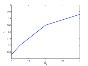
As an illustration of these results, for $P_{2}=0.1$ and $\delta=\frac{m}{n}=0.75$ using Theorems 2 and 1 and combining the exponents with the combinatorial exponent, we have calculated the threshold for $P_{1}$ for different values of $w_{2}$ in the range $[1,3]$ , below which the signal can be recovered. The curve is depicted in Figure 1. As expected, the curve is suggesting that in this setting weighted $\ell_{1}$ minimization boosts the weak threshold in comparison with $\ell_{1}$ minimization. This is verified in the next section by some examples.

V Simulation

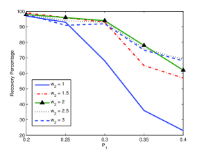
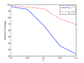
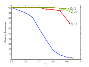
We demonstrate by some examples that appropriate weights can boost the recovery percentage. We fix $P_{2}$ and $n=2m=200$, and try $\ell_{1}$ and weighted $\ell_{1}$ minimization for various values of $P_{1}$. We choose $n_{1}=n_{2}=\frac{n}{2}$ Figure 2a shows one such comparison for $P_{2}=0.05$ and different values of $w_{2}$. Note that the optimal value of $w_{2}$ varies as $P_{1}$ changes. Figure 2b illustrates how the optimal weighted $\ell_{1}$ minimization surpasses the ordinary $\ell_{1}$ minimization. The optimal curve is basically achieved by selecting the best weight of Figure 2a for each single value of $P_{1}$. Figure 3 shows the result of simulations in another setting where $P_{2}=0.1$ and $m=0.75n$ (similar to the setting of the previous section). It is clear from the figure that the recovery success threshold for $P_{1}$ has been shifted higher when using weighted $\ell_{1}$ minimization rather than standard $\ell_{1}$ minimization. Note that this result very well matches the theoretical result of Figure 1.

References

- [1] David Donoho, “High-Dimensional Centrally Symmetric Polytopes with Neighborliness Proportional to Dimension ”, Discrete and Computational Geometry , 102(27), pp. 617-652, 2006, Springer .
- [2] Emmanuel Candes and Terence Tao, “Decoding by linear programming”, IEEE Trans. on Information Theory, 51(12), pp. 4203 - 4215, December 2005.
- [3] David Donoho and Jared Tanner, “Neighborliness of randomly-projected simplices in high dimensions”, Proc. National Academy of Sciences, 102(27), pp. 9452-9457, 2005.
- [4] W. Xu and Babak Hassibi, “Compressed Sensing Over the Grassmann Manifold: A Unified Analytical Framework,” Forty-Sixth Annual Allerton Conference, September 23-26.
- [5] Mark Davenport, Michael Wakin, and Richard Baraniuk, “Detection and estimation with compressive measurements”, Rice ECE Department Technical Report TREE 0610, November 2006
- [6] Shihao Ji, Ya Xue, and Lawrence Carin, “Bayesian compressive sensing,” IEEE Trans. on Signal Processing, 56(6) pp. 2346 - 2356, June 2008
- [7] M. Stojnic, F. Parvaresh and B. Hassibi, “On the reconstruction of block-sparse signals with an optimal number of measurements”, Preprint 2008.
- [8] E. J. Cand s, M. Wakin and S. Boyd. Enhancing sparsity by reweighted l1 minimization. J. Fourier Anal. Appl., 14 877-905
- [9] Branko Grünbaum, Grassmann angles of convex polytopes. Acta Math., 121:pp.293-302, 1968.
- [10] Branko Grünbaum, Convex polytopes, volume 221 of Graduate Texts in Mathematics. Springer-Verlag, New York, second edition, 2003. Prepared and with a preface by Volker Kaibel, Victor Klee and GnterüM. Ziegler.
- [11] L.A.Santaló, Geometría integral en espacios de curvatura constante, Rep.Argetina Publ.Com.Nac.Energí Atómica, Ser.Mat 1,No.1(1952)
- [12] Peter McMullen. “Non-linear angle-sum relations for polyhedral cones and polytopes”. Math. Proc. Cambridge Philos. Soc., 78(2):pp.247-261, 1975.
- [13] M. Stojnic, W. Xu, and B. Hassibi, “Compressed sensing - probabilistic analysis of a null-space characterization”, IEEE International Conference on Acoustics, Speech and Signal Processing, Pages:3377-3380, March 31 2008-April 4 2008.
- [14] http://www.dsp.ece.rice.edu/cs/