Comparison of high-accuracy numerical simulations of black-hole binaries with stationary phase post-Newtonian template waveforms for Initial and Advanced LIGO.

Abstract

We study the effectiveness of stationary-phase approximated post-Newtonian waveforms currently used by ground-based gravitational-wave detectors to search for the coalescence of binary black holes by comparing them to an accurate waveform obtained from numerical simulation of an equal-mass non-spinning binary black hole inspiral, merger and ringdown. We perform this study for the Initial- and Advanced-LIGO detectors. We find that overlaps between the templates and signal can be improved by integrating the match filter to higher frequencies than used currently. We propose simple analytic frequency cutoffs for both Initial and Advanced LIGO, which achieve nearly optimal matches, and can easily be extended to unequal-mass, spinning systems. We also find that templates that include terms in the phase evolution up to 3.5 pN order are nearly always better, and rarely significantly worse, than 2.0 pN templates currently in use. For Initial LIGO we recommend a strategy using templates that include a recently introduced pseudo-4.0 pN term in the low-mass ($M\leq 35\,M_{\odot}$) region, and 3.5 pN templates allowing unphysical values of the symmetric reduced mass $\eta$ above this. This strategy always achieves overlaps within 0.3% of the optimum, for the data used here. For Advanced LIGO we recommend a strategy using 3.5 pN templates up to $M=12\,M_{\odot}$, 2.0 pN templates up to $M=21\,M_{\odot}$, pseudo-4.0 pN templates up to $65\,M_{\odot}$, and 3.5 pN templates with unphysical $\eta$ for higher masses. This strategy always achieves overlaps within 0.7% of the optimum for Advanced LIGO.

1 Introduction

The coalescence of binary black holes is one the most promising sources of gravitational waves for interferometric gravitational-wave detectors, such as LIGO, Virgo and GEO600 [1]. The first-generation LIGO detectors have achieved their design sensitivity and recorded over one year of coincident data [2]. This data, together with data from the Virgo detector, are currently being searched for gravitational waves from compact binary coalescence [3, 4, 5, 6, 7, 8]. Upgrades to improve the sensitivity of these detectors by a factor of two, and ultimately 10, are underway. Optimal searches using the enhanced detectors in 2009 will be sensitive to black-hole coalescence out to hundreds of megaparsecs [9]. The advanced detectors, operational next decade, could detect black-hole binaries at distances of over 1 Gpc [10].

Optimal searches for gravitational waves use matched filtering, which requires accurate knowledge of the waveform [1]. Previous searches in LIGO data have used post-Newtonian and phenomenological templates to search for the coalescence of black-hole binaries [5, 6, 8]. Over the last several years numerical relativity has made remarkable breakthroughs in simulating the late inspiral, merger and ringdown of black-hole binaries. The computational cost of these simulations is high, however, making it impractical to use them directly as template waveforms for use in a matched-filter search. It has been shown that there is good agreement between the waveforms generated by numerical relativity with analytic post-Newtonian waveforms to within just a few orbits of merger [11, 12, 13, 14, 15, 16, 17, 18, 19, 20, 21].

This paper uses the high-accuracy Caltech–Cornell numerical-relativity waveforms to suggest improvements to the analytic waveforms currently used in gravitational-wave searches by LIGO and Virgo. A similar study has been performed by Pan et al. using numerical data from Pretorius and the Goddard groups [13]. Our main results are in agreement with their conclusion that a simple extension of the existing stationary-phase approximation to the adiabatic post-Newtonian waveforms (called TaylorF2 in Ref. [22]) yields high overlaps with numerical waveforms.

In Sec. 2, we review the current techniques used for searching for gravitational waves in gravitational-wave detector data. We discuss the construction of the waveform—a pN–NR hybrid—in Sec. 3. In Sec. 4 we employ the hybrid waveform in a comparison of the detection efficiency of gravitational-wave templates that may be used in upcoming searches of LIGO and Virgo data. Finally, in Sec. 5, we discuss improvements that may be made to the current data-analysis techniques to optimize overlaps.

Throughout this paper, we use only the $(l,m)=(2,2)$ component of the waveform $\Psi_{4}^{2,2}$ (as defined, e.g., in [19]). For convenience, we drop the superscript. Whenever possible, we use dimensionless quantities, like $r\,M\,|\Psi_{4}|$, where $r$ is the areal radius of the observation sphere, and $M$ is the total apparent-horizon mass of the holes in the initial data. However, for any calculation involving the LIGO noise curve, we have a physical scale, and thus use standard mks units.

2 Searches for gravitational waves from black-hole binaries

2.1 Matched filtering

Current searches for gravitational waves from binary black-hole coalescence use matched filtering to search for a waveform buried in noise. The matched filter is the optimal filter for detecting a signal in stationary Gaussian noise. Suppose that $n(t)$ is a stationary Gaussian noise process with one-sided power spectral density $S_{n}(f)$ given by $\langle\tilde{n}(f)\tilde{n}^{\ast}(f^{\prime})\rangle=\frac{1}{2}S_{n}(|f|)\delta(f-f^{\prime})$. For long integration times, the data stream $s(t)$ output by the detector will always be dominated by the noise. Thus, we can simply approximate $n\approx s$ to calculate $S_{n}(f)$.

Using this power spectral density (PSD), we can define the inner product between two real-valued signals—the data stream $s$ and the filter template $h$—by

$$\left({s}\,\mskip 1.0mu\vrule\mskip 1.0mu\,{h}\right) \equiv 2\,\Re\int_{-\infty}^{\infty}\,\frac{\tilde{s}(f)\,\tilde{h}^{\ast}(f)}{S_{n}(|f|)}\,df$$ (1)

$$=4\,\Re\int_{0}^{\infty}\,\frac{\tilde{s}(f)\,\tilde{h}^{\ast}(f)}{S_{n}(f)}\,df\ .$$ (2)

Then, given data $s$ which may contain either noise $n$ or noise and a gravitational wave signal $h$,

$$s=\left\{\begin{array}[]{l}n\\ n+h\end{array}\right.\ ,$$ (3)

the matched-filter signal-to-noise ratio (SNR) is defined as

$$\rho=\frac{1}{\sqrt{\left({h}\,\mskip 1.0mu\vrule\mskip 1.0mu\,{h}\right)}}\left({s}\,\mskip 1.0mu\vrule\mskip 1.0mu\,{h}\right)\ .$$ (4)

The SNR can then be used to construct a detection statistic (directly or in combination with other statistics). It is therefore important to ensure that the templates used in searches accurately model the expected waveforms to avoid reduction in the value of $\rho$. The overlap between two templates $h$ and $h^{\prime}$ is defined as

$$\Braket{h}{h^{\prime}}\equiv\frac{\left({h}\,\mskip 1.0mu\vrule\mskip 1.0mu\,{h^{\prime}}\right)}{\sqrt{\left({h}\,\mskip 1.0mu\vrule\mskip 1.0mu\,{h}\right)\left({h^{\prime}}\,\mskip 1.0mu\vrule\mskip 1.0mu\,{h^{\prime}}\right)}}\ .$$ (5)

The overlap encodes the fractional loss in SNR that results from using the template $h^{\prime}$ rather than the true waveform $h$. In a search that uses $\rho$ as a detection statistic this corresponds to the fractional loss in distance to which the search is sensitive.

The filter template includes arbitrary time and phase offsets, encoded by the arrival time and phase, $t_{\mathrm{a}}$ and $\phi_{\mathrm{a}}$. Under a change of these quantities, the Fourier transform behaves as

$$\tilde{h}(f)\to\tilde{h}(f)\,\rme^{-2\pi ift_{\mathrm{a}}-i\phi_{\mathrm{a}}}\ .$$ (6)

We maximize over these two variables by calculating the inner product as

$$\max_{t_{\mathrm{a}},\phi_{\mathrm{a}}}\,\left({s}\,\mskip 1.0mu\vrule\mskip 1.0mu\,{h}\right) =\max_{t_{\mathrm{a}},\phi_{\mathrm{a}}}\,4\,\Re\int_{0}^{\infty}\,\frac{\tilde{s}(f)\,\tilde{h}^{\ast}(f)}{S_{n}(f)}\,\rme^{2\pi ift_{\mathrm{a}}+i\phi_{\mathrm{a}}}\,df$$ (7)

$$=4\max_{t_{\mathrm{a}}}\,\left|\int_{0}^{\infty}\,\frac{\tilde{s}(f)\,\tilde{h}^{\ast}(f)}{S_{n}(f)}\,\rme^{2\pi ift_{\mathrm{a}}}\,df\right|\ .$$ (8)

Note that this integral is just the (inverse) Fourier transform of the quantity $\tilde{s}(f)\,\tilde{h}^{\ast}(f)/S_{n}(f)$ evaluated at $t_{\mathrm{a}}$. Thus finding the maximum over $t_{\mathrm{a}}$ involves taking the Fourier transform and selecting the largest element of the finite set that results from discretization.

In this paper we are concerned with overlaps between pN waveforms and NR signals; to weight the inner product we use the following PSDs for Initial and Advanced LIGO: for Initial LIGO we use an analytic approximation to the LIGO design PSD given by

$$S_{n}(f) = 3.136\times 10^{-4}\bigg{[}\left(\frac{4.49f}{150.0}\right)^{-56.0}$$ (9)

$$+ 0.16\left(\frac{f}{150}\right)^{-4.52}+\left(\frac{f}{150.0}\right)^{2}+0.52\bigg{]}$$

All integrals start from 40 Hz. As shown in Fig. 4, at this frequency the noise is an order of magnitude higher than its lowest value, and below this frequency it rises rapidly as $\sim f^{-56}$. The region below 40 Hz therefore contributes very little signal power to the SNR [6]. The PSD for Enhanced LIGO, which will begin operation in mid 2009, has a similar shape to that for Initial LIGO although it has a factor of $\sim 2$ increase in strain sensitivity. Our results using the Initial-LIGO PSD are therefore valid for Enhanced LIGO, as the sensitivity factor cancels in Eq. (5); overlaps depend on the shape of the PSD.

For Advanced LIGO we use the GWINC program [23] to generate the PSD. Bench reports the PSD in increments of 0.0124 Hz. When calculating discrete integrals against signals sampled at other frequencies we obtain values for the PSD by linearly interpolating between the values provided by Bench. We start integrals at 10 Hz as that is the point where the noise has increased by two orders of magnitude above its minimum, as also shown in Fig. 4.

2.2 Post-Newtonian template

Searches for gravitational waves in LIGO and Virgo use a post-Newtonian waveform known asTaylorF2 [8]. This is a frequency-domain waveform obtained via the stationary-phase approximation [24], which assumes that the frequency-domain amplitude is simply proportional to $f^{-7/6}$ (the lowest-order behavior), while its phasing is given by the phase of the time-domain waveform, as a function of frequency. For a binary consisting of masses $m_{1}$ and $m_{2}$, located at an “effective” distance $D_{\mathrm{eff}}$, we have

$$\tilde{h}(f;M,\eta,f_{c})=\Theta(f_{c}-f)\,\left(\frac{1\,\mathrm{Mpc}}{D_{\mathrm{eff}}}\right)\,{\mathcal{A}}_{1\,\mathrm{Mpc}}(M,\eta)\,f^{-7/6}\,\rme^{i\varphi(f;M,\eta)}\ ,$$ (10)

where

$${\mathcal{A}}_{1\,\mathrm{Mpc}}(M,\eta) = \left(\frac{5\pi}{24}\right)^{1/2}\left(\frac{GM_{\odot}/c^{2}}{1\,\mathrm{Mpc}}\right)\times$$ (11)

$$\times\left(\frac{\pi GM_{\odot}}{c^{3}}\right)^{-1/6}\left(\frac{\eta}{M_{\odot}}\right)^{1/2}\left(\frac{M}{M_{\odot}}\right)^{1/3}\ ,$$

and the phasing $\varphi$ of the frequency-domain waveform is given to 3.5pN accuracy by the formula [25, 26]

$$\varphi(f;M,\eta) = 2\pi ft_{0}-2\phi_{0}-\pi/4$$ (12)

$$+\frac{3}{128\eta}\Bigg{[}v^{-5}+\left(\frac{3715}{756}+\frac{55}{9}\eta\right)v^{-3}-16\pi v^{-2}$$

$$+\left(\frac{15\,293\,365}{508\,032}+\frac{27\,145}{504}\eta+\frac{3085}{72}\eta^{2}\right)v^{-1}$$

$$+\pi\left[\frac{38\,645}{756}-\frac{65}{9}\eta\right]\left[1+3\ln\left(\frac{v}{v_{0}}\right)\right]$$

$$+\left[\frac{11\,583\,231\,236\,531}{4\,694\,215\,680}-\frac{640}{3}\pi^{2}-\frac{6\,848}{21}\gamma\right]v$$

$$+\bigg{[}\left(-\frac{15\,335\,597\,827}{3\,048\,192}+\frac{2\,255}{12}\pi^{2}-\frac{47\,324.0}{63.0}-\frac{794\,8}{9}\right)\eta$$

$$\qquad+\frac{76\,055}{1\,728}\eta^{2}-\frac{127\,825}{1\,296}\eta^{3}\bigg{]}v$$

$$+\pi\left[\frac{77\,096\,675}{254\,016}+\frac{378\,515}{1\,512}\eta-\frac{74\,045}{756}\eta^{2}\right]v^{2}\Bigg{]}\ .$$

where $v=\left(\frac{GM}{c^{3}}\pi f\right)^{1/3}$, $M=m_{1}+m_{2}$ and $\eta=m_{1}m_{2}/(m_{1}+m_{2})^{2}$.

The overall frequency scale is set by the total mass $M$, as can be seen by observing that each occurrence of $f$ is accompanied by a factor of $M$. Thus, going to a higher-mass system shifts the waveform to lower frequencies. On the other hand, to first order, the timescale for the rate of change of the frequency is given by the chirp mass:

$$\mathcal{M}\equiv\left(\frac{m_{1}^{3}\,m_{2}^{3}}{m_{1}+m_{2}}\right)^{1/5}=M\,\eta^{3/5}\ .$$ (13)

Clearly, the total mass and chirp mass give us two very different handles on the behavior of the waveform. These two handles will be important when we try to match the template to our waveform in regions where the post-Newtonian and stationary-phase approximations are poor. This is typically the case for high-mass systems, which only enter the detector band late in the inspiral. In this case, we can still obtain a high match, at the cost of using templates with the wrong values of $M$ and $\eta$.

We also note that physical binary systems are restricted to $0<\eta\leq 1/4$. However, for higher values of $\eta$, the formulas shown above still give plausible waveforms; in fact, in some cases these templates match the true waveform better than any physical template. We will explore the implications of allowing unphysical values for $\eta$ in searches over the templates in Sec. 4.2.

Note the Heaviside function in Eq. (10). This contains a cutoff frequency $f_{c}$ which is used to ensure that the template does not extend to frequencies much greater than the frequencies contained in the expected signal. This is essentially a third parameter for the template waveform, and will be searched over. See Sec. 4.1 for a discussion of strategies for optimizing detection by changing this cutoff.

Frequencies which are often used to characterize coalescing binary black holes are: (i) the frequency at the innermost stable circular orbit (ISCO), $r=6M$, around a single Schwarzschild black hole with the total mass of the binary system; (ii) the frequency at the light ring, $r=3.0/M$, around a single Schwarzschild black hole with the total mass of the binary system; (iii) the ringdown frequency of the final black hole, which depends on both its spin and mass; and (iv) an “effective ringdown,” $f_{\mathrm{ERD}}\equiv 1.07\,f_{\mathrm{Ringdown}}$ defined in [13].

Current searches use 2pN stationary-phase approximation (SPA) TaylorF2 templates [8]. It has previously been shown that such waveforms provide acceptable detection templates for binary neutron stars and sub-solar mass black holes [27], but not necessarily for higher-mass black holes. This is an issue we will investigate below by testing 2pN and 3.5pN templates.

3 PN–NR hybrid waveform

In order to perform our comparison we need to construct a “true” black-hole binary waveform, which we might expect to observe with detectors. A numerical simulation will provide the data for the crucial nonlinear merger phase. We carefully extract the data and extrapolate it to large radius, and investigate the effects of numerical error on the final result. Because this waveform is very computationally expensive to produce, it covers only about 32 cycles, which is not sufficient for a thorough investigation of the possibility of detecting it in searches of data from gravitational-wave detectors. Thus, we match the numerical waveform to a post-Newtonian waveform, producing a hybrid which extends for many thousands of cycles, covering the entire band of interest.

3.1 Numerical simulation, extraction, and extrapolation

The numerical simulation is the same as that described in Refs. [16, 28]: an equal-mass, non-spinning, black-hole binary with reduced eccentricity [29], beginning roughly 16 orbits before merger, continuing through merger and ringdown [28]. It is performed with the Caltech–Cornell pseudospectral code, using boundary conditions designed to prevent constraint violations and gravitational radiation from entering the domain [30, 31].

Data is extracted from the simulation in the form of the Newman–Penrose scalar

$$\Psi_{4}=-C_{\alpha\beta\gamma\delta}l^{\alpha}\bar{m}^{\beta}l^{\gamma}\bar{m}^{\delta}\ ,$$ (14)

where $l^{\alpha}$ and the complex vector $\bar{m}^{\beta}$ are constructed with reference to the coordinate basis. Along the positive $z$ axis, we have

$$l^{\alpha} = \frac{1}{\sqrt{2}}\,\left(t^{\alpha}-z^{\alpha}\right)\ ,$$ (15)

$$\bar{m}^{\beta} = \frac{1}{\sqrt{2}}\,\left(\frac{\partial}{\partial x}-i\,\frac{\partial}{\partial y}\right)^{\beta}\ .$$ (16)

Here, $t^{\alpha}$ is the timelike unit normal to the spatial hypersurface, and $z^{\alpha}$ is the unit vector in the positive $z$ direction. The vectors $\partial/\partial x$ and $\partial/\partial y$ are the standard coordinate vectors, which are not normalized. $\Psi_{4}$ is extracted as a function of time, at various radii along the positive $z$ axis. This is then extrapolated to large radii, as described in Ref. [16], and in greater detail in Ref. [32].

The measured (instantaneous) frequency at the beginning of the simulation is

$$f_{\mathrm{initial}}=(1.08\pm 0.01)\times 10^{3}\,\mathrm{Hz}\,\frac{M_{\odot}}{M}\ .$$ (17)

The measured ringdown frequency is

$$f_{\mathrm{ringdown}}=(1.78\pm 0.02)\times 10^{4}\,\mathrm{Hz}\,\frac{M_{\odot}}{M}\ .$$ (18)

The measured Christodoulou mass and spin of the final black hole are

$$M_{\chi\mathrm{,final}} = (0.95162\pm 0.00002)\,M_{\chi\mathrm{,initial}}\ ,$$ (19)

$$S_{\mathrm{final}} = (0.68646\pm 0.00004)\,M^{2}_{\chi\mathrm{,final}}\ .$$ (20)

Using this value for the spin, a quasi-analytic formula due to Echeverria [33] predicts a value of $1.77\times 10^{4}\,\mathrm{Hz}\,\frac{M_{\odot}}{M}$, for the ringdown frequency, in close agreement with the measured frequency.

3.2 Accuracy of the numerical simulation

The numerical waveform will be the standard against which we will judge the TaylorF2 waveforms used in LIGO data analysis. To understand how precisely we should trust our final results, we need to understand the accuracy of the waveform itself. The most obvious measure of the error in this fiducial waveform is its convergence with increasing numerical resolution. Fig. 1 shows the overlap (Eq. (5)) between waveforms computed at different resolutions. The data used here are the extrapolated $\Psi_{4}$ waveforms, integrated in time twice.

Figure 1: Convergence testing for numerical waveforms from a data-analysis perspective, using the match between waveforms computed at different numerical resolutions. The waveforms are scaled to various masses, and the Initial-LIGO noise curve is used in the calculation of the match. The upper panel shows the overlap without maximization over arrival time and phase; the lower panel shows the overlap after maximization. In each panel, the lower (dashed) line compares the lowest- and highest-resolution simulations, while the upper (solid) line compares the medium- and highest-resolution simulations. Note that this plot uses only numerical data, with no post-Newtonian contribution.

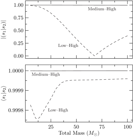
Because of the short extent of the numerical waveforms, we need to be careful when using their Fourier transforms. The signal can be corrupted easily by the non-periodicity of the waveforms, and the discontinuous jumps that result. For Fig. 1 we mitigate this problem by increasing the sampling frequency of the input data, and restricting the Fourier transform to frequencies corresponding to instantaneous frequencies contained in the data. The input data can easily be upsampled in the time domain by interpolating the phase and amplitude of the complex data to a finer time grid. We then perform the transform, and explicitly set the data to zero at frequencies below $f_{\mathrm{initial}}$ and above $f_{\mathrm{ringdown}}$, as given in Eqs. 17 and 18. While the results do depend on whether or not we impose these cutoffs, they do not depend sensitively on the actual cutoff frequencies.

The overlap between the lowest- and highest-resolution simulations (dashed lines) actually passes through zero, as shown in the upper panel. Presumably, this is because of loss of phase accuracy over the course of the simulation. All three simulations begin with the same initial data, so the waveforms are most similar at the beginning. Masses for which this is the most important segment (the lowest masses) will naturally have the highest overlap between resolutions. As the simulation progresses, numerical error accumulates—notably in the phase—so the overlap decreases with masses for which later segments dominate the overlap (higher masses). When the overlap is optimized over arrival time and phase, we can see that the overlap becomes much better, as shown in the lower panel, indicating sufficient accuracy within any frequency band for which phase coherence is required. In either case, the medium and highest resolutions are much more nearly the same. Without optimization, their overlap is within a few tenths of a percent of 1; after optimization, the overlap is within $10^{-6}$ of 1.

In the rest of our analysis we use the highest-resolution waveform. Because we always optimize over arrival time and phase, the lower panel of Fig. 1 is the most relevant, and shows that the waveform has converged to very high accuracy. The overlaps we quote below will only be given to three decimal places at most, because this is roughly the accuracy of the single-precision numerical methods used in the rest of the paper. This accuracy is also sufficient for searches of gravitational-wave data. Thus, the truncation error of the simulated waveform is irrelevant for those purposes.

Other sources of error include residual eccentricity and spin, the influence of the outer boundary of the simulation, extrapolation errors, and coordinate effects, as discussed in Ref. [16]. The eccentricity had a disproportionately large effect on the error quoted in that paper because of the matching technique, which is not used here. Restricting attention to the other effects of eccentricity, the uncertainty falls below that due to numerical error. Similarly, using the techniques of Ref. [34], the initial spins of the black holes have been measured more reliably, and found to be more than an order of magnitude smaller than previously determined, allowing us to reduce the estimate for that error to less than the numerical truncation error. The various coordinate effects were all estimated to be of roughly the same magnitude as the numerical error.

With the numerical error being many times more accurate than needed for this analysis, and the other sources of uncertainty being of roughly the same size, these considerations indicate that the overall error in our fiducial waveform is substantially less than the precision needed for this analysis.

3.3 Hybrid waveform

Numerical simulations cannot simulate a very large portion of the inspiral of a black-hole binary system. Indeed, the longest such simulation currently in the literature is the one used here—which extends over just 32 gravitational wave cycles before merger. Fortunately, this is the only stage in which simulations are needed. It has been shown previously [16] that the TaylorT4 waveform with 3.5-pN phase and 3.0-pN amplitude matches the early part of this simulation to very high accuracy. We generate a TaylorT4 waveform of over 8000 gravitational wave cycles ($t\sim 1.2\times 10^{6}M$, starting at $Mf=0.004$), and transition between the two to create a hybrid. This long waveform is sufficient to ensure that—even for the lowest-mass systems we will consider—the waveform begins well before it enters the frequency band of interest to LIGO.

We begin with $\Psi_{4}$ data, which will later be integrated to obtain $h$. Following Ref. [19], we match the numerical waveform to the pN waveform by adjusting the time and phase offsets of the pN waveform to minimize the quantity

$$\Xi(\Delta t,\Delta\phi)=\int_{t_{1}}^{t_{2}}\,\left[\phi_{\mathrm{NR}}(t)-\phi_{\mathrm{pN}}(t-\Delta t)-\Delta\phi\right]^{2}\,dt\ .$$ (21)

Here, we choose $t_{1}=900\,M$ and $t_{2}=1730\,M$, which is closer to the beginning of the waveform than in the previous paper. This particular interval is chosen to begin and end at troughs of the small oscillations due to the residual eccentricity $e\sim 5\times 10^{-5}$ in our numerical waveform. Taking a range from trough to trough or peak to peak—rather than node to node, for example—of the eccentricity effects minimizes their influence on the matching. The eccentricity oscillations can be seen more easily after low-pass filtering the waveform, though we find filtering to be unnecessary for this paper. The junk radiation apparent in the waveform as shown here has no effect on the resulting match—as we have verified by filtering, and redoing the match. Because the final waveform will incorporate no numerical data before $t_{1}$ and very little immediately thereafter (as explained below), the junk radiation will have no effect on any of our results—as we have also explicitly verified. In particular, by integrating $\Psi_{4}$ to obtain $h$, we will effectively smooth the junk radiation.

Figure 2: Amplitude and phase differences between the numerical and post-Newtonian waveforms, $\Psi_{4}$, that are blended to create the hybrid waveform. The vertical lines at $900M$ and $1730M$ denote the region over which matching and hybridization occur. Note that the agreement is well within the numerical accuracy of the simulation, represented by the horizontal bands, throughout the matching region. Also note that the phase difference is fairly flat for a significant period of time after the matching range, which indicates that the match is not sensitive to the particular range chosen for matching.

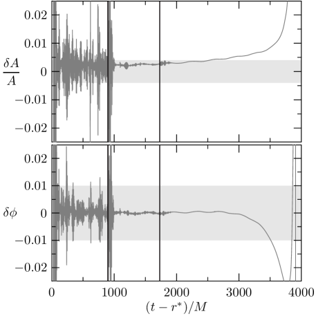
In Fig. 2 we compare the phase of the numerical and pN waveforms. The quantities plotted are

$$\delta\phi \equiv \phi_{\mathrm{pN}}-\phi_{\mathrm{NR}}\ ,$$ (22)

$$\frac{\delta A}{A} \equiv \frac{A_{\mathrm{pN}}-A_{\mathrm{NR}}}{A_{\mathrm{NR}}}\ ,$$ (23)

shown over the interval on which both data sets exist. The vertical bars denote the matching region. Note that the phase difference is well within the accuracy of the simulation (about 0.01 radians, represented by the horizontal band) over a range extending later than the matching region. Also, the difference between the two is fairly flat, which implies that the match is not very sensitive to the region chosen for matching. Because of this, we expect that the phase coherence between the early pN data and the late NR data will be physically accurate to high precision.

The hybrid waveform is then constructed by blending the two matched waveforms together according to

$$A_{\mathrm{hyb}}(t) = \tau(t)\,A_{\mathrm{NR}}+\left[1-\tau(t)\right]\,A_{\mathrm{pN}}(t)\ ,$$ (24)

$$\phi_{\mathrm{hyb}}(t) = \tau(t)\,\phi_{\mathrm{NR}}+\left[1-\tau(t)\right]\,\phi_{\mathrm{pN}}(t)\ .$$ (25)

The blending function $\tau$ is defined by

$$\tau(t)=\left\{\begin{array}[]{ll}0&\mathrm{if}\quad t<t_{1}\\ \frac{t-t_{1}}{t_{2}-t_{1}}&\mathrm{if}\quad t_{1}\leq t<t_{2}\\ 1&\mathrm{if}\quad t_{2}\leq t\end{array}\right.$$ (26)

The values of $t_{1}$ and $t_{2}$ are the same as those used for the matching. The amplitude discrepancy between the pN waveform and the NR waveform over this interval is within numerical uncertainty—roughly $0.4\%$. As with the matching technique (Eq. (21)), this method is similar to that of Ref. [35], but distinct, in that we blend the phase and amplitude, rather than the real and imaginary parts. This leads to a smoothly blended waveform, shown in Fig 3.

Figure 3: The last $t=5000M_{\odot}$ of the hybrid waveform used in this analysis: the $h_{+}$ waveform seen by an observer on the positive $z$ axis. The vertical lines denote the matching and hybridization region. The $0$ on the time axis corresponds to the beginning of data from the numerical simulation.

Up to this point, the waveform has been $\Psi_{4}$ data. With the long waveform in hand, we numerically integrate twice to obtain $h$, and set the four integration constants so that the final waveform has zero average and first moment [29]. Because of the very long duration of the waveforms, this gives a reasonable result, which is only incorrect at very low frequencies—lower than any frequency of interest to us. We have also checked that our results do not change when we effectively integrate in the frequency domain by taking

$$\tilde{h}=-\frac{\tilde{\Psi}_{4}}{4\,\pi\,f^{2}}\ ,$$ (27)

which is the frequency-domain analog of the equation $\Psi_{4}=\ddot{h}$.

4 Detection efficiency of gravitational-wave templates

We now compare the signal described in the previous section to restricted, stationary phase TaylorF2 post-Newtonian templates with terms up to order 2.0, order 3.5, and a “pseudo-4.0 pN-order” term recommended in Ref. [13]. Overlaps are calculated using the techniques of Sec. 2.1, with the signal $s$ being the hybrid waveform described in Sec. 3 scaled to a range of masses. We consider both the Initial- and Advanced-LIGO noise curves.

Plots of the hybrid waveforms in comparison to the Initial-LIGO noise curve are shown in Fig. 4.

Figure 4: Hybrid Caltech–Cornell waveform scaled to various total masses, with sources optimally oriented and placed at 100 Mpc, shown against the Initial- and Advanced-LIGO noise curves. Markers are placed along the lines at frequencies corresponding to various instantaneous frequencies of the waveforms. The triangles represent the beginning and end of the blending region; the circle represents the ISCO frequency; the square the light-ring; and the diamond the measured ringdown frequency. See the text for discussion of the normalization. The values given for $\rho$ use the Initial-LIGO noise curve, with sources at a distance of 100 Mpc.

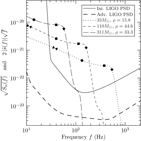
The masses are chosen so that various frequencies of interest (the final stitching frequency, the ISCO, and the ringdown) occur at the “seismic wall” for Initial LIGO: 40 Hz. The waveforms $\tilde{s}$ are scaled to depict the detectability of the signal, typically quantified by the SNR introduced in  (4), which may be written as

$$\rho^{2}\equiv\int_{0}^{\infty}\frac{4\,\tilde{s}(f)\,\tilde{s}^{\ast}(f)}{S_{n}(f)}\,df=\int_{0}^{\infty}\frac{\left|2\,\tilde{s}(f)\,\sqrt{f}\right|^{2}}{S_{n}(f)}\,d\ln{f}\ .$$ (28)

In the final expression, the numerator and denominator have the same units, and are directly comparable. Because the square root of the denominator is familiar, we plot that along with the square root of the numerator. Plotting these two quantities together gives a graphical impression of the detectability of the waveform, and the relative importance of each part of the waveform, by its height above the noise curve. In Ref. [36], Brady and Creighton define a slightly different quantity, the characteristic strain $h_{\mathrm{char}}\equiv f\,|\tilde{s}(f)|\ .$ The relative factor of $\sqrt{f}$ they use is present so that they can plot $h_{\mathrm{char}}$ against $\sqrt{f\,S_{n}(f)}$. Cutler and Thorne [37] define still another quantity, the signal strength $\tilde{h}_{s}(f)$, which is related to the Fourier transform by $\tilde{h}(f)=\sqrt{5}\,\frac{T}{N}\,\tilde{h}(s)\ .$ The factor of $\sqrt{5}$ comes from averaging over the orientation of the binary, which we do not do. $T/N$ is the ratio of the threshold to the rms noise at the endpoint of signal processing.

For each template family we initially optimize over signal mass $M$, symmetric mass ratio $\eta=m_{1}m_{2}/(m_{1}+m_{2})^{2}$, and upper cutoff frequency $f_{c}$. The optimization is performed using a Nelder–Mead (“amoeba”) algorithm [38]. The amoeba starts with a simplex in the parameter space, and proceeds through a series of steps, each of which will improve the value of the function at at least one vertex. The algorithm terminates when all vertices have converged to the same point to within a specified tolerance. This process is deterministic, and amounts to an enhanced steepest-ascent algorithm. It is therefore only guaranteed to find a local maximum, and indeed we find that an amoeba instance started at a random point in the parameter space is most likely to converge to a point that does not give the highest possible overlap. We interpret this as being due to a large region in parameter space containing a local maximum and a relatively smaller region containing the global maximum. We therefore supplement the basic amoeba by running 300 instances with random starting values, and taking the best match obtained over all instances. In repeated runs the same optimal parameters were found by at least some of the amoebas, which supports the claim that this is the true maximum.

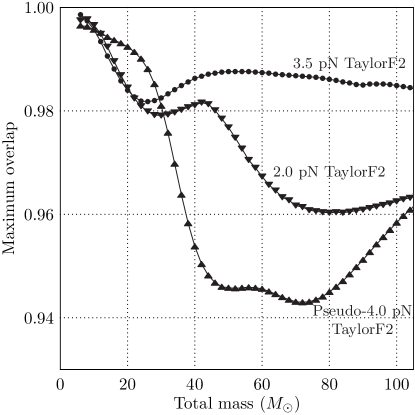
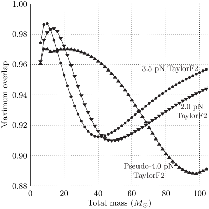
The results of optimizing over all of $M,\eta$ and $f_{c}$ for selected masses for Initial LIGO are given in Table 1 and summarized in Fig. 5. For Initial LIGO, in the range covered by the current Compact Binary Coalescence (CBC) low-mass search $(M<35M_{\odot})$ [8], the pseudo-4.0 pN TaylorF2 waveforms achieve the highest overlaps, exceeding those obtained with 3.5 pN waveforms by $\sim 1\%$. Above $35M_{\odot}$ the 3.5 pN waveforms produce overlaps as much as 4% greater than those obtained with pseudo-4.0 pN waveforms over a range from $40$–$80M_{\odot}$. With the Advanced-LIGO noise curve, in the CBC low-mass range, the 3.5 pN and pseudo-4.0 pN waveforms produce overlaps within 2% of each other, with 3.5 pN producing higher overlaps below 20 $M_{\odot}$ and pseudo-4.0 pN producing higher overlaps in the range $20$–$35M_{\odot}$. Pseudo-4.0 pN continues to give the highest overlaps up to $60M_{\odot}$, producing overlaps as much as 4% greater than those obtained with 3.5 pN waveforms. Above $60M_{\odot}$ 3.5 pN waveforms again yield the best overlaps, by as much as 6% around 90 $M_{\odot}$.

	$(10+10)M_{\odot}$	$(20+20)M_{\odot}$	$(30+30)M_{\odot}$	$(50+50)M_{\odot}$
$\Braket{s^{\textrm{NR-CC}}}{h^{\textrm{SPA}_{c}^{\textrm{ext}}(2.0)}}$	0.99	0.98	0.97	0.96
$M/M_{\odot}$	$23.27^{+0.13}_{-0.12}$	$25.99^{+0.61}_{-0.56}$	$35.22^{+1.84}_{-1.89}$	$47.52^{+6.87}_{-4.73}$
$\eta$	$0.199^{+0.0030}_{-0.0030}$	$0.771^{+0.0490}_{-0.0420}$	$1.000_{-0.1390}$	$1.000_{-0.2490}$
$f_{\mathrm{cut}}$ (Hz)	$501.18^{+523.00}_{-153.00}$	$431.35^{+358.00}_{-77.00}$	$296.05^{+53.00}_{-31.00}$	$190.56^{+20.00}_{-14.00}$
$\Braket{s^{\textrm{NR-CC}}}{h^{\textrm{SPA}_{c}^{\textrm{ext}}(3.5)}}$	0.98	0.99	0.99	0.99
$M/M_{\odot}$	$18.75^{+0.10}_{-0.10}$	$31.88^{+0.77}_{-0.71}$	$47.15^{+4.37}_{-3.27}$	$259.89^{+0.00}_{-194.18}$
$\eta$	$0.290^{+0.0040}_{-0.0040}$	$0.493^{+0.0530}_{-0.0410}$	$0.756^{+0.2440}_{-0.2290}$	$0.954^{+0.0460}_{-0.2090}$
$f_{\mathrm{cut}}$ (Hz)	$506.50^{+518.00}_{-155.00}$	$448.80^{+576.00}_{-83.00}$	$324.74^{+145.00}_{-42.00}$	$197.17^{+24.00}_{-16.00}$
$\Braket{s^{\textrm{NR-CC}}}{h^{\textrm{SPA}_{c}^{\mathcal{Y}}(4)}}$	0.99	0.96	0.95	0.96
$M/M_{\odot}$	$23.64^{+0.13}_{-0.12}$	$47.90^{+1.28}_{-1.13}$	$61.81^{+8.68}_{-6.19}$	$89.93^{+20.44}_{-16.60}$
$\eta$	$0.182^{+0.0030}_{-0.0030}$	$0.181^{+0.0160}_{-0.0140}$	$0.523^{+0.4260}_{-0.1820}$	$0.529^{+0.4720}_{-0.3100}$
$f_{\mathrm{cut}}$ (Hz)	$509.47^{+654.00}_{-145.00}$	$352.44^{+73.00}_{-61.00}$	$309.53^{+72.00}_{-47.00}$	$195.63^{+21.00}_{-15.00}$

Table 1: Maximum overlaps between Caltech–Cornell hybrid waveforms and restricted stationary-phase pN templates using the Initial-LIGO noise curve. The first number in each block is the overlap; subsequent numbers are the template parameters that achieve this overlap. Parameter values within the specified ranges keep the overlap within 1% of the maximum by varying that parameter, while leaving others fixed. We restrict the search to $0\leq\eta\leq 1.000$, so the upper error bounds when $\eta\sim 1.000$ may be artificially small.

	$(10+10)M_{\odot}$	$(20+20)M_{\odot}$	$(30+30)M_{\odot}$	$(50+50)M_{\odot}$
$\Braket{s^{\textrm{NR-CC}}}{h^{\textrm{SPA}_{c}^{\textrm{ext}}(2.0)}}$	0.98	0.92	0.91	0.94
$M/M_{\odot}$	$25.15^{+0.02}_{-0.02}$	$47.73^{+0.12}_{-0.11}$	$54.39^{+0.51}_{-0.43}$	$60.19^{+1.55}_{-1.29}$
$\eta$	$0.170^{+0.0010}_{-0.0010}$	$0.188^{+0.0010}_{-0.0010}$	$0.335^{+0.0080}_{-0.0070}$	$0.891^{+0.0660}_{-0.0490}$
$f_{\mathrm{cut}}$ (Hz)	$444.77^{+132.00}_{-115.00}$	$267.64^{+48.00}_{-50.00}$	$262.44^{+34.00}_{-36.00}$	$182.41^{+24.00}_{-18.00}$
$\Braket{s^{\textrm{NR-CC}}}{h^{\textrm{SPA}_{c}^{\textrm{ext}}(3.5)}}$	0.97	0.92	0.92	0.96
$M/M_{\odot}$	$20.27^{+0.02}_{-0.02}$	$38.11^{+0.11}_{-0.09}$	$50.09^{+0.49}_{-0.42}$	$78.10^{+1.89}_{-1.50}$
$\eta$	$0.245^{+0.0010}_{-0.0010}$	$0.277^{+0.0020}_{-0.0020}$	$0.386^{+0.0130}_{-0.0100}$	$0.494^{+0.0760}_{-0.0330}$
$f_{\mathrm{cut}}$ (Hz)	$355.85^{+97.00}_{-88.00}$	$262.83^{+47.00}_{-48.00}$	$281.34^{+41.00}_{-37.00}$	$186.31^{+30.00}_{-19.00}$
$\Braket{s^{\textrm{NR-CC}}}{h^{\textrm{SPA}_{c}^{\mathcal{Y}}(4)}}$	0.97	0.96	0.94	0.90
$M/M_{\odot}$	$22.24^{+0.02}_{-0.02}$	$46.57^{+0.11}_{-0.11}$	$72.06^{+0.35}_{-0.35}$	$118.50^{+1.99}_{-1.63}$
$\eta$	$0.208^{+0.0010}_{-0.0010}$	$0.190^{+0.0010}_{-0.0010}$	$0.177^{+0.0020}_{-0.0030}$	$0.186^{+0.0100}_{-0.0070}$
$f_{\mathrm{cut}}$ (Hz)	$473.49^{+551.00}_{-136.00}$	$353.18^{+73.00}_{-69.00}$	$242.43^{+37.00}_{-36.00}$	$152.16^{+19.00}_{-19.00}$

Table 2: Maximum overlaps between Caltech–Cornell hybrid waveforms and restricted stationary-phase pN templates using the Advanced-LIGO noise curve. The first number in each block is the overlap; subsequent numbers are the template parameters that achieve this overlap. Parameter values within the specified ranges keep the overlap within 1% of the maximum by varying that parameter, while leaving others fixed. We restrict the search to $0\leq\eta\leq 1.000$, so the upper error bounds when $\eta\sim 1.000$ may be artificially small.

A significant feature of Tables 1 and 2 is the size of the error bars on the cutoff frequencies. For $M=20M_{\odot}$ the cutoff frequency can vary as much as 128% above and 28% below the optimal value while losing no more than 1% of overlap. This leads us to consider the range of possible template parameters which may give high overlaps. In the next section we consider the reduction in overlap as the parameters $f_{c}$ and $\eta$ are independently varied from the optimal value.

Figure 5: Left: Overlaps between Caltech–Cornell hybrid waveforms, scaled to various masses, and restricted stationary-phase pN waveforms for Initial-LIGO PSD. Optimization is over $M$ and $\eta$, which the cutoff frequency $f_{c}$ is prescribed by the weighted average described below. The mass ratio $\eta$ is allowed to range over unphysical values. The best-fit values found for the pseudo-4.0 pN templates are always physical in this case. See Sec. 4.2. Right: The same, for the Advanced-LIGO PSD

4.1 Effect of upper frequency cutoff

As shown in Fig. 4 the amplitude of the NR waveforms drops sharply at around the lightring frequency, which depends on the total mass of the binary. The TaylorF2 waveforms do not model the late inspiral, merger or ringdown and hence will continue to evolve as $f^{-7/6}$ at all frequencies, increasingly deviating from the NR waveform. This suggests that the upper frequency cutoff of the TaylorF2 waveform should be chosen to be below the frequency at which the two diverge. However, the effect of the divergence is mitigated by the PSD. The denominator of the overlap, Eq. (5), depends on $\left({s}\,\mskip 1.0mu\vrule\mskip 1.0mu\,{s}\right)$ which is a constant, and $\left({h}\,\mskip 1.0mu\vrule\mskip 1.0mu\,{h}\right)$ which would increase without limit if not for the PSD. Fig. 6 shows $|\tilde{h}(f)|^{2}/S_{n}(f)$—the integrand of $\left({h}\,\mskip 1.0mu\vrule\mskip 1.0mu\,{h}\right)$—for the Initial-LIGO noise curve for an example TaylorF2 waveform for an equal-mass $10\,M_{\odot}$ binary. We see that above about 450 Hz there is very little contribution to the integrand, and so extending the cutoff frequency above this will not impact the overlap.

Figure 6: Left: Integrand of Eq. (1) for a TaylorF2, 3.5 pN waveform with $M=10$ and $\eta=0.25$, at a distance of 100 Mpc, using the Initial-LIGO noise curve. Note that the shape of this curve does not change as we change $M$ and $\eta$; only the vertical scale changes. Right: Overlap between Caltech–Cornell waveform scaled to $M=40\,M_{\odot}$ and restricted TaylorF2, 3.5 pN waveform using the best-match values for $M$ and $\eta$, as a function of the cutoff frequency $f_{c}$, with the Initial-LIGO noise curve. The vertical bars are meant to delineate 1% loss. Note that the upper bound extends to higher frequencies indefinitely.

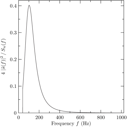
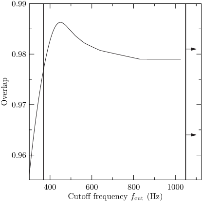
The numerator of the overlap, $\left({s}\,\mskip 1.0mu\vrule\mskip 1.0mu\,{h}\right)$, can only increase as the cutoff frequency is raised, however frequencies above the lightring where the waveforms have diverged will contribute very little. The effect of including higher frequencies on the overlap is therefore determined by the $\left({h}\,\mskip 1.0mu\vrule\mskip 1.0mu\,{h}\right)$ term in the denominator. For systems with ringdown frequencies well above the peak of the integrand in Fig. 6, this term will not significantly reduce the overlap. For example, binaries of total mass roughly $40\,M_{\odot}$ have ringdown frequencies at roughly 450 Hz. Only a small fraction of the SNR comes from higher frequencies. Thus, we expect that systems with lower masses should not suffer great loss in overlap if the cutoff frequency is higher than ringdown. However for higher-mass systems the overlap can be significantly reduced if the upper frequency cutoff is too large. This is indeed what we find, as shown by a representative example on the right in Fig. 6. For this $40\,M_{\odot}$ system, using the Initial-LIGO noise curve, the optimal cutoff frequency is around 450 Hz—roughly the ringdown frequency. Decreasing the cutoff quickly decreases the overlap. The cutoff may be increased almost indefinitely, however, with only 0.5% loss in overlap. This, of course, changes when using the Advanced-LIGO noise curve. We revisit this issue in Sec. 5.

4.2 Unrestricted $\eta$

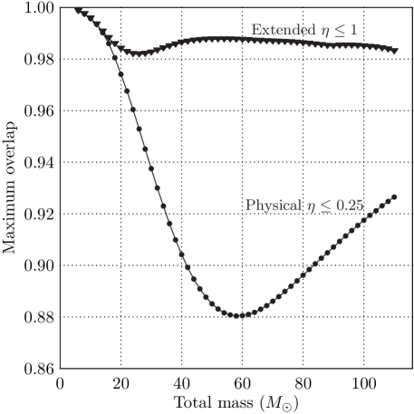
The physical symmetric mass ratio is restricted to the range $0<\eta\leq 0.25$, values above this imply complex-valued masses. However the pN waveforms are well-behaved for $0<\eta<1.0$, and as seen from Tables 1 and 2, the highest overlaps are often obtained at unphysical values of $\eta$. In Fig. 7 we show the effect of limiting the optimization to physical $\eta$. At high masses, the limitation reduces the optimal overlap by up to 12%. TaylorF2 waveforms with $\eta\leq 1/4$ would not be expected to accurately model the late-inspiral and merger part of the waveform, as non-Newtonian effects are increasingly significant in this region. We find that allowing unphysical $\eta$ broadens the space of waveforms covered by the TaylorF2 approximation sufficiently to capture more of the late-inspiral and merger.

Figure 7: Maximum overlaps obtained by allowing $\eta$ to range over unphysical values, compared to those obtained by restricting the range of $\eta$. These overlaps are generated using 3.5 pN TaylorF2 templates, searching over values of the total mass and mass ratio. Extending to unphysical values of $\eta$ improves the match by up to 11%.

5 Recommendations for improvements

Based on the analysis of the previous sections we propose a series of adjustments to searches using TaylorF2 template waveforms to enhance the efficiency of those searches. First, as seen in Fig. 5 for Initial LIGO, adding terms up to 3.5 pN order produces overlaps as large or larger than the current 2.0 pN templates over most of the mass range, while the pseudo-4.0 pN templates recommended in Ref. [13] produce slightly larger overlaps at masses near $20\,M_{\odot}$. Thus, we recommend pseudo-4.0 pN templates for the low mass range, $M<35M_{\odot}$, and 3.5 pN templates for higher masses. The improvement due to 3.5 pN templates over 2.0 pN generally holds for Advanced LIGO as well. The 3.5 pN templates produce larger overlaps than 2.0 pN templates above $50\,M_{\odot}$ without a significant loss (within 1%) at lower masses. However, there is a large region for which the pseudo-4.0 pN term does significantly better. When using an Advanced-LIGO noise curve, we recommend 3.5 pN templates generally, 2.0 pN templates in the range $12$–$21\,M_{\odot}$ and pseudo-4.0 pN templates for masses in the range $21$–$65\,M_{\odot}$.

As a second improvement, we note from Fig. 7 that allowing $\eta$ to range over unphysical values significantly improves matches with 3.5 pN templates above $30\,M_{\odot}$. In preliminary studies we have found that extending to $\eta\leq 1$ roughly doubles the size of the template bank, and the advantages must therefore be weighed against the increase in false alarm rate.

Figure 8: Left: Candidate $f_{c}$ values for 3.5 pN templates with Initial LIGO. The dark gray band contains cutoff frequencies with matches within 1% of the value at which the best overlap was obtained. The light gray band contains frequencies with matches within 3%. Right: Candidate $f_{c}$ values for 3.5 pN templates with Advanced LIGO. The dark gray band contains cutoff frequencies with matches within 1% of the value at which the best overlap was obtained. The light gray band contains frequencies with matches within 3%. Note that the weighted-average cutoff extends past the 1% error bars for $12<M/M_{\odot}<40$. However, in that same region, the 3.5 pN templates do poorly overall, and we recommend pseudo-4.0 pN templates. The optimal cutoff frequency for pseudo-4.0 pN templates is much closer to the weighted-average cutoff in this mass range.

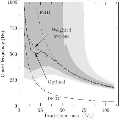
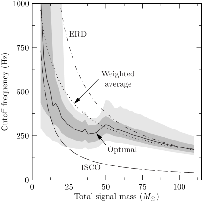
Our third recommendation involves the cutoff frequency used for the template waveform. Optimization over the cutoff frequency is too computationally intensive to be done in searches. Currently, the cutoff frequency is typically taken to be the Schwarzschild ISCO frequency. To examine the effect of this choice we vary $f_{c}$ while keeping the mass and $\eta$ at their optimal values, for each of the signal masses in our range. The result of one such variation is shown in Fig. 6 (right). Figs. 8 shows the variations for all masses, highlighting the regions within which the overlap drops by less than 1% (dark gray) and 3% (light gray) of the optimal value. This figure also shows the ISCO and ERD frequencies, neither of which stays within the 1% band for both Initial and Advanced LIGO. In particular, the ISCO is a poor choice for both Initial and Advanced LIGO except at very low masses, where the precise value of the cutoff is almost irrelevant.

The ISCO is often pointed to—somewhat arbitrarily—as a good estimate of the breakdown of post-Newtonian approximations [39]. So, for instance, if we were to match a pN template to a physical waveform, beginning at some point in the distant past, we might expect them to separate quite badly near the ISCO. Of course, for realistic black-hole binaries, the gravitational waves will only enter the LIGO band late in the inspiral—just before the ISCO for low-mass systems, or after the ISCO for high-mass systems. We can see from Fig. 4 that, for masses below about $30\,M_{\odot}$, the ISCO is high enough that lower-frequency parts of the waveform contribute the most to the SNR. For very high masses, however, this basically cuts the waveform down to nothing. In Initial LIGO, the ISCO is completely buried in seismic noise for masses above about $100\,M_{\odot}$. Thus, we must move the cutoff frequency up. We cannot push the cutoff far above ringdown, because the physical waveform simply ceases to exist (see Fig. 4). It has been suggested that an “effective ringdown” (ERD) frequency $f_{\mathrm{ERD}}\equiv 1.07\,f_{\mathrm{Ringdown}}$ is a useful upper limit [13]. For intermediate masses, we would like to interpolate somehow between these two extremes of ISCO and ERD. We suggest setting the cutoff frequency to a weighted average of the two, where the weights are the contributions to the SNR below the given frequency. If we assume coherent phasing between the template and the physical waveform, we can simply take the amplitudes of the two waveforms. Also, note that the restricted SPA approximation for the amplitude is reasonable. Thus, define

$$\rho_{\mathrm{ISCO}}^{2} \equiv \int_{0}^{f_{\mathrm{ISCO}}}\,\frac{f^{-7/3}}{S_{n}(f)}\,df\ ,$$ (29)

$$\rho_{\mathrm{ERD}}^{2} \equiv \int_{f_{\mathrm{ISCO}}}^{f_{\mathrm{ERD}}}\,\frac{f^{-7/3}}{S_{n}(f)}\,df\ ,$$ (30)

$$\rho_{\mathrm{tot}}^{2} \equiv \int_{0}^{f_{\mathrm{ERD}}}\,\frac{f^{-7/3}}{S_{n}(f)}\,df\ ,$$ (31)

$$f_{\mathrm{cut}} \equiv \frac{f_{\mathrm{ISCO}}\ \rho_{\mathrm{ISCO}}+f_{\mathrm{ERD}}\ \rho_{\mathrm{ERD}}}{\rho_{\mathrm{tot}}}\ .$$ (32)

We have already dropped constant factors in the expressions for $\rho$ that will cancel out.

Note that these expressions only depend on the total mass by way of the limits of integrations—which are very simple, known functions of the mass—so these integrals could be done just once for a given noise curve, storing the intermediate values. When the cutoff needs to be calculated, the cumulative integral could be evaluated at the given ISCO and ringdown frequencies. Hence, this would be a fast way of calculating the cutoff, with no need to do the integrals each time the cutoff is needed.

We can test this recommended frequency by comparing it to the optimal cutoff frequency found by the amoeba search described in Sec. 4. For 3.5 pN templates in Initial LIGO, we find that it is an excellent match to the optimal frequency. Fig. 8 shows these two values, along with dark and light bands showing the regions in which changing $f_{c}$ results in a loss of overlap of 1% and 3%, respectively. Of course, the same figure shows that using the ERD recommendation would stay within the 1% error bounds. Nonetheless, the close match between this recommendation and the true optimum suggests that it is sound. Thus, our final recommendation is to use the weighted-average frequency cutoff throughout the entire mass range. While our analysis has been restricted to equal-mass systems, the cutoff frequency we have defined here could be applied to unequal-mass systems as well. It will be interesting to see how this cutoff fares in those situations.

Similar results hold for Advanced LIGO, when using our recommended template for each mass. That is, in regions where 3.5 pN templates do poorly (see Fig. 5), the weighted average is a poor predictor of the optimal cutoff frequency using those templates, as shown in Fig. 8. However, in those same regions—where pseudo-4.0 pN templates do well—the weighted average is a good predictor of the optimal cutoff frequency for 4.0 pN templates. Thus, again, we recommend using the weighted-average frequency cutoff throughout the entire mass range with Advanced LIGO.

By prescribing a cutoff frequency, the search does not need to extend over that parameter. Similarly, by prescribing a post-Newtonian order, we need use only one template for a given total mass. On the other hand, if these recommendations decrease the overlap found by too much when using them compared to the overlap found by an unconstrained search, it may be better to search the larger parameter space. We can evaluate the loss in overlap by comparing the results found using our recommendations to the results found when searching over the set of all three template families, and all masses, mass ratios, and cutoff frequencies. We have determined that this loss in overlap when using our recommendations is always less than 0.0025 for Initial LIGO, and less than 0.007 for Advanced LIGO.

6 Conclusions

We have compared high-accuracy NR waveforms for equal-mass binary black holes from the Caltech–Cornell group to stationary phase post-Newtonian waveforms. We examined a number of factors that influence the matches between the two, with the goal of optimizing the matches and hence improving the efficiency of templated searches in Initial and Advanced LIGO. We first considered the effect of the post-Newtonian order to which the phase evolution is taken, and found that adding terms up to 3.5 pN or pseudo-4.0 pN to the currently-used 2.0 pN templates significantly improves the matches over a large range of masses, as shown in Fig. 5. We then studied the effect of varying the upper cutoff frequency of the templates. The frequency that achieves the optimal match is a function of mass, and we find this function is well-approximated by an average between ISCO and ERD, weighted by contribution to the SNR, as shown in Fig. 8. Finally, we allow the symmetric mass ratio $\eta$ to range over unphysical values up to $1.0$, and find that this dramatically improves matches, as shown in Fig. 7. Based on the results we recommend adjusting the searches using TaylorF2 template waveforms by going up to 3.5 pN or 4.0 pN over most of the mass range, integrating up to our recommended cutoff, and allowing allowing $\eta$ to extend up to 1. For Initial LIGO, the overlaps obtained using these parameters is always within 0.0025 of overlaps achievable by optimizing over all three parameters.

In future work we plan to extend this analysis to unequal-mass and spinning black-hole systems. We have found that allowing unphysical values of $\eta$ roughly doubles the size of the template bank, and we also plan to study the impact of this on the false alarm rate.

References

- [1] Thorne K S 1987 Three hundred years of gravitation ed Hawking S W and Israel W (Cambridge: Cambridge University Press)
- [2] Abbott B et al. (LIGO Scientific Collaboration) 2007 (Preprint arXiv:0711.3041)
- [3] Abbott B et al. (LIGO Scientific Collaboration) 2004 Phys. Rev. D 69 122001
- [4] Abbott B et al. (LIGO Scientific Collaboration) 2005 Phys. Rev. D 72 082001
- [5] Abbott B et al. (LIGO Scientific) 2005 Phys. Rev. D 72 082002
- [6] Abbott B et al. (LIGO Scientific Collaboration) 2008 Phys. Rev. D 77 062002
- [7] Abbott B et al. (LIGO Scientific) 2008 Phys. Rev. D 78 042002
- [8] Abbott B et al. (LIGO Scientific) 2009 (Preprint arXiv:0901.0302)
- [9] Adhikari R, Fritschel P and Waldman S 2006 Enhanced LIGO Tech. Rep. LIGO-T060156-01-I URL http://www.ligo.caltech.edu/docs/T/T060156-01.pdf
- [10] Fritschel P 2003 (Preprint gr-qc/0308090)
- [11] Buonanno A, Cook G B and Pretorius F 2007 Phys. Rev. D 75 124018
- [12] Baker J G, van Meter J R, McWilliams S T, Centrella J and Kelly B J 2007 Phys. Rev. Lett. 99 181101
- [13] Pan Y, Buonanno A, Baker J G, Centrella J, Kelly B J, McWilliams S T, Pretorius F and van Meter J R 2008 Phys. Rev. D 77 024014
- [14] Buonanno A, Pan Y, Baker J G, Centrella J, Kelly B J, McWilliams S T and van Meter J R 2007 Phys. Rev. D 76 104049
- [15] Hannam M, Husa S, González J A, Sperhake U and Brügmann B 2008 Phys. Rev. D 77 044020
- [16] Boyle M, Brown D A, Kidder L E, Mroué A H, Pfeiffer H P, Scheel M A, Cook G B and Teukolsky S A 2007 Phys. Rev. D 76 124038
- [17] Gopakumar A, Hannam M, Husa S and Brügmann B 2008 Phys. Rev. D 78 064026
- [18] Hannam M, Husa S, Brügmann B and Gopakumar A 2007 Phys. Rev. D 78 104007
- [19] Boyle M, Buonanno A, Kidder L E, Mroué A H, Pan Y, Pfeiffer H P and Scheel M A 2008 Phys. Rev. D 78 104020
- [20] Mroué A H, Kidder L E and Teukolsky S A 2008 Phys. Rev. D 78 044004
- [21] Hinder I, Herrmann F, Laguna P and Shoemaker D 2008 (Preprint arXiv:0806.1037)
- [22] Damour T, Iyer B R and Sathyaprakash B S 2001 Phys. Rev. D 63 044023 erratum: [40]
- [23] GWINC: Gravitational Wave Interferometer Noise Calculator (v1 default parameters) URL http://lhocds.ligo-wa.caltech.edu:8000/advligo/GWINC
- [24] Cutler C and Flanagan E E 1994 Phys. Rev. D 49 2658–2697
- [25] L. Blanchet, B. R. Iyer, and B. Joguet 2002 Phys. Rev. D 65 061501 erratum: [41]
- [26] L. Blanchet, T. Damour, G. Esposito-Farèse and B.R. Iyer 2004 Phys. Rev. Lett. 93 191101
- [27] Droz S, Knapp D J, Poisson E and Owen B J 1999 Phys. Rev. D 59 124016
- [28] Scheel M A, Boyle M, Chu T, Kidder L E, Matthews K D and Pfeiffer H P 2008 (Preprint arxiv:0810.1767)
- [29] Pfeiffer H P, Brown D A, Kidder L E, Lindblom L, Lovelace G and Scheel M A 2007 Class. Quantum Grav. 24 S59–S81
- [30] Holst M, Lindblom L, Owen R, Pfeiffer H P, Scheel M A and Kidder L E 2004 Phys. Rev. D 70 084017
- [31] Lindblom L, Scheel M A, Kidder L E, Owen R and Rinne O 2006 Class. Quantum Grav. 23 S447–S462
- [32] Boyle M and Mroué A H 2008 In preparation
- [33] Echeverria F 1989 Phys. Rev. D 40 3194
- [34] Lovelace G, Owen R, Pfeiffer H P and Chu T 2008 Phys. Rev. D 78 084017
- [35] Ajith P, Babak S, Chen Y, Hewitson M, Krishnan B, Sintes A M, Whelan J T, Brügmann B, Diener P, Dorband N, Gonzalez J, Hannam M, Husa S, Pollney D, Rezzolla L, Santamaría L, Sperhake U and Thornburg J 2008 Phys. Rev. D 77 104017
- [36] Brady P R and Creighton J D 2002 Encyclopedia of Physical Science and Technology vol 7 (Academic Press, Inc) pp 33–48 3rd ed ISBN 978-0122274107
- [37] Cutler C and Thorne K S 2002 Proceedings of the GR16 Conference on General Relativity and Gravitation (World Scientific)
- [38] Press W H, Teukolsky S A, Vetterling W T and Flannery B P 2007 Numerical Recipes: The Art of Scientific Computing 3rd ed (Cambridge University Press)
- [39] Blanchet L 2006 Living Rev. Rel. 9 4
- [40] Damour T, Iyer B R and Sathyaprakash B S 2005 Phys. Rev. D 72 029902
- [41] L. Blanchet, B. R. Iyer, and B. Joguet 2005 Phys. Rev. D 71 129902