Biases and Uncertainties in Physical Parameter Estimates of Lyman Break Galaxies from Broad-band Photometry

Abstract

We investigate the biases and uncertainties in estimates of physical parameters of high-redshift Lyman break galaxies (LBGs), such as stellar mass, mean stellar population age, and star formation rate (SFR), obtained from broad-band photometry. These biases arise from the simplifying assumptions often used in fitting the spectral energy distributions (SEDs). By combining $\rm{\Lambda}$CDM hierarchical structure formation theory, semi-analytic treatments of baryonic physics, and stellar population synthesis models, we construct model galaxy catalogs from which we select LBGs at redshifts $z$ $\sim$ 3.4, 4.0, and 5.0. The broad-band photometric SEDs of these model LBGs are then analysed by fitting galaxy template SEDs derived from stellar population synthesis models with smoothly declining SFRs. We compare the statistical properties of LBGs’ physical parameters – such as stellar mass, SFR, and stellar population age – as derived from the best-fit galaxy templates with the intrinsic values from the semi-analytic model. We find some trends in these distributions: first, when the redshift is known, SED-fitting methods reproduce the input distributions of LBGs’ stellar masses relatively well, with a minor tendency to underestimate the masses overall, but with substantial scatter. Second, there are large systematic biases in the distributions of best-fit SFRs and mean ages, in the sense that single-component SED-fitting methods underestimate SFRs and overestimate ages. We attribute these trends to the different star formation histories predicted by the semi-analytic models and assumed in the galaxy templates used in SED-fitting procedure, and to the fact that light from the current generation of star-formation can hide older generations of stars. These biases, which arise from the SED-fitting procedure, can significantly affect inferences about galaxy evolution from broadband photometry.

1 Introduction

Over the last decade, astronomy has experienced a boom of panchromatic surveys of high redshift galaxies – such as the Great Observatories Origins Deep Survey (GOODS, Giavalisco et al., 2004a) and the Cosmic Evolution Survey (COSMOS, Scoville et al., 2007) – thanks to the developments of space telescopes, like Hubble Space Telescope (HST) and Spitzer Space Telescope ($Spitzer$), and also of ground-based facilities, including Keck observatory, Very Large Telescope (VLT), and Subaru telescope. Spectral energy distributions (SEDs) constructed from the photometric data of wide wavelength coverage have been used to constrain galaxy parameters, such as stellar masses, SFRs, and stellar population ages, of high redshift galaxies via comparison with simple stellar population synthesis models (e.g. Papovich et al., 2001; Shapley et al., 2001, 2005; Shim et al., 2007; Stark et al., 2007; Verma et al., 2007). Accompanied byselection techniques to separate high-redshift galaxy samples efficiently via their broad-band colors and magnitudes, these surveys have provided increasing information about the nature of high-redshift galaxies.

However, despite recent advances in our knowledge of the properties of high redshift galaxies, more accurate estimation of physical parameters is necessary for addressing several important issues in galaxy evolution and cosmology. For example, it is as yet uncertain whether the Lyman break galaxies (LBGs, Steidel et al., 1996; Giavalisco, 2002) – high-redshift, star-forming galaxies selected according to their rest-frame ultraviolet (UV) colors – will evolve into large ellipticals (Adelberger et al., 1998; Steidel et al., 1998), or into smaller spheroids, such as small ellipticals/spiral bulges or subgalactic structures, which will later be merged to form larger galaxies at $z\sim 0$ (Lowenthal et al., 1997; Sawicki & Yee, 1998; Somerville et al., 2001). Accurate knowledge of physical parameters, such as stellar masses and SFRs, serves as one of the important elements in discriminating among the possible evolutionary descendants of LBGs. Also, accurately constraining LBG’s stellar-population ages and stellar masses is necessary for determining how much the LBG populations contributed to cosmic reionization. Better estimation of these parameters is also crucial in comparing different galaxy populations at different redshifts.

The stellar populations of LBGs as well as other populations of high-redshift galaxies have been studied by several authors using SED-fitting methods to compare the photometric SEDs of observed galaxies with various galaxy spectra from stellar population synthesis models. Papovich et al. (2001) investigated 33 spectroscopically-confirmed LBGs with a redshift range, $2.0\leq z\leq 3.5$. They found that the mean lower limit of stellar masses of these LBGs is $\sim 6\times 10^{9}$ $M_{\sun}$ with upper limits of $\sim$ 3-8 times larger and that the mean age is $\sim$ 120 Myr (assuming solar metallicity and Salpeter (1955) IMF) with broad range between 30 Myr and 1 Gyr. More importantly, they concluded that the most robust parameter constrained through SED-fitting is stellar mass, while stellar population age and especially star formation rate (SFR) are only poorly constrained. Also, they speculated that SED-fitting methods (single-component fitting) can only give lower limits to galaxies’ stellar masses because the results from the SED-fitting methods are largely driven by the light from the most massive, most recently formed stars. Shapley et al. (2001) studied the physical parameters of 74, $z\sim$ 3 LBGs with spectroscopic redshifts. They confirmed that among various physical parameters, stellar mass is the most tightly constrained, and that constraints on other parameters such as dust extinction and age are weak. With the assumption of solar metallicity and a Salpeter IMF, the median age (defined as time since the onset of current star formation) was found to be $t_{sf}\sim$ 320 Myr with a large spread from several Myr to more than 1 Gyr. The median stellar mass was 1.2$\times 10^{10}~{}h^{-2}~{}M_{\sun}$, which is higher than the Papovich et al. (2001) value. However, the Shapley et al. (2001) LBGs were generally brighter than LBGs in the Papovich et al. (2001) sample. The two studies found similar stellar masses for LBGs with similar rest-frame UV luminosities. Shapley et al. (2001) also found that about 20 $\%$ of the LBGs have best-fit ages older than 1 Gyr, stellar masses larger than $10^{10}~{}M_{\sun}$, and SFR $\sim$ 30 $M_{\sun}$ $yr^{-1}$, and they interpreted these as galaxies which have formed their stars over a relatively long period in a quiescent manner. Shapley et al. (2001) also noted that more luminous galaxies are dustier than less luminous ones and that younger galaxies are dustier and have higher SFR.

More recently, Verma et al. (2007) studied 21 $z\sim$ 5 LBGs, six of which have confirmed spectroscopic redshifts and the remaining 15 of which have photometric redshifts. These LBGs were found to be moderately massive with median stellar mass $\sim$ $2\times 10^{9}$ $M_{\sun}$, and to have high SFRs with a median of $\sim$ 40 $M_{\sun}\rm{yr^{-1}}$. They also found that the stellar mass estimates are the most robust of all derived properties. Best-fit ages have a large spread with a median value $\sim$ 25 Myr, assuming a metallicity of one-fifth solar (0.2 $Z_{\sun}$) and a Salpeter IMF. Verma et al. (2007) also compared their $z\sim$ 5 LBGs with Shapley et al. (2001)’s $z\sim$ 3 LBGs, assuming the same IMF and metallicity (i.e. solar metallicity and Salpeter IMF), and concluded that these two samples of LBGs with similar rest-frame UV luminosity are clearly different. Specifically, $z\sim$ 5 LBGs are much younger ($\lesssim$ 100 Myr) and have lower stellar masses ($\sim~{}10^{9}~{}M_{\sun}$) than $z\sim$ 3 LBGs. The fraction of young (age $<$ 100 Myr) galaxies is $\sim$ $70\%$ for $z\sim$ 5 LBGs while it is $\sim$ $30\%$ for $z\sim$ 3 LBGs. They also concluded that these $z\sim$ 5 LBGs are the likely progenitors of the spheroidal components of present-day massive galaxies, based on their high stellar mass surface densities. Stark et al. (2007) analysed 72 $z\sim$ 5 galaxies (not just LBGs) with photometric redshifts. They performed an SED-fitting analysis on a spectroscopically confirmed subset of 14 $z\sim$ 5 galaxies to derive best-fit stellar masses ranging between $3\times 10^{8}$ and $2\times 10^{11}$ $M_{\sun}$, and ages from 1 Myr to 1.1 Gyr. Three out of these 14 galaxies have stellar masses in excess of $10^{11}~{}M_{\sun}$. Using stellar mass estimates from both spectroscopically confirmed and candidate galaxies, they calculated a stellar mass density at $z\sim$ 5 of $6~{}\times~{}10^{6}~{}M_{\sun}~{}\rm{Mpc^{-3}}$, which is much larger than the integration of the star formation rate density (SFRD) from $z\sim$ 10 to 5. They attributed this discrepancy either to significant dust extinction or to undetected low-luminosity star-forming galaxies at z $\gtrsim$ 5. Shim et al. (2007) studied the properties of 1088 massive LBGs whose best-fit stellar masses are larger than $10^{11}~{}M_{\sun}$ at $z\sim$ 3. They derived stellar masses of these massive LBGs through SED-fitting with the assumption of a Salpeter IMF, and noted that LBGs which are detected in mid-infrared wavelength are the ones with large stellar mass and severe dust extinction among LBG population.

The SED-fitting method is also used to constrain physical parameters for high-z Lyman-$\alpha$ emitting galaxies (LAEs, Finkelstein et al., 2007) and for submillimetre galaxies (Dye et al., 2008). Finkelstein et al. (2007) analysed $z\sim 4.5$ LAEs through SED fitting and found their ages range from 1 Myr to 200 Myr (assuming a constant star formation history), and stellar masses from $2\times 10^{7}-2\times 10^{9}$ $M_{\sun}$. Dye et al. (2008) used SED fitting to study physical parameters of SCUBA (Submillimetre Common-User Bolometer Array) sources, finding an average stellar mass of $\sim 10^{11.8\pm 0.1}M_{\sun}$.

However, the estimated parameter values and implications derived from these values are prone to several sources of error including errors inherent in SED-fitting methods. It is unclear whether or not SED-fitting methods deliver biased estimates of parameters such as stellar mass, age, and SFR. It is also unclear how much worse the parameter estimates become if spectroscopic redshifts are unavailable and the photometric data must be used to constrain not only the star formation history, but also the redshift. The critical question is how far we can trust the physical parameters derived using mainly photometric data under the assumption of simple star-formation histories (SFHs), when real galaxies are expected to have more complex formation/evolution histories with several possible episodes of star-formation.

In this paper, we address this issue by comparing the statistical distributions of intrinsic physical parameters of model Lyman break galaxies (LBGs) from semi-analytic models (SAMs) of galaxy formation, with the estimates of those same parameters derived from stellar population synthesis models through the commonly used SED-fitting method.

There have been several studies which tried to constrain the stellar populations of LBGs or of high-redshift galaxies by comparing them with predictions from theoretical models, such as semi-analytic models (e.g. Somerville et al., 2001; Idzi et al., 2004) or cosmological hydrodynamic simulations (e.g. Nagamine et al., 2005; Night et al., 2006; Finlator et al., 2007). Somerville et al. (2001) compared $z\sim 3$ and $z\sim 4$ observed LBGs with semi-analytic models to investigate possible scenarios for LBGs, and Idzi et al. (2004) put constraints on the properties of $z\sim 4$ LBGs through comparison of colors of observed LBGs and SAMs model LBGs. Nagamine et al. (2005) and Night et al. (2006) used cosmological simulations to place constraints on properties of UV-selected, $z\sim 2$ galaxies and $z\sim 4-6$ LBGs. Finlator et al. (2007) constructed a set of galaxy templates from hydrodynamical simulations and used them to place constraints on properties of 6 $z\leq 5.5$ observed galaxies. Our approach is distinct from these studies. Here, instead of comparing model galaxies with observed ones, we perform SED fitting on model galaxies, derive best-fit parameters, and compare them with the intrinsic values given in the model, trying to understand quantitatively as well as qualitatively the biases and uncertainties of SED-fitting methods in constraining the physical parameters of LBGs.

To accomplish this, we construct galaxy formation histories by combining $\rm{\Lambda}$CDM hierarchical structure formation theory with semi-analytic treatments of gas cooling, star formation, supernova feedback, and galaxy mergers. Then, using the stellar population synthesis models of Bruzual $\&$ Charlot (Bruzual & Charlot, 2003, hereafter BC03), and a simple model for dust extinction, we derive the photometric properties of these model galaxies. After selecting LBGs through appropriate color criteria, we compare the photometric spectral energy distributions (SEDs) in observed-frame optical (HST/ACS) through mid-infrared ($Spitzer$/IRAC) passbands of these model LBGs with those of SED templates from stellar population synthesis model of BC03 using a $\chi^{2}$-minimization method. In this SED-fitting procedure, a large multi-parameter space is explored to minimize any prior. Each parameter – such as star-formation time scale, age, dust-extinction, and metallicity – in this parameter space spans a broad as well as physically realistic range. The distributions of physical parameters of these model LBGs derived from this SED-fitting method are compared with the input distributions of these parameters from the semi-analytic model.

Various parameters in the semi-analytic model are calibrated to reproduce the colors of observed LBGs in the southern field of the GOODS (GOODS-S). The GOODS (Giavalisco et al., 2004a) is a deep, multiwavelength survey which covers a combined area of $\sim 320$ $\rm{arcmin^{2}}$ in two fields – GOODS-N centered on the Hubble Deep Field-North (HDF-N), and GOODS-S centered on the Chandra Deep Field-South (CDF-S). The extensive wavelength coverage of the photometric data in the GOODS fields including HST/ACS (${\it Advanced~{}Camera~{}for~{}Surveys}$) and $Spitzer$/IRAC (${\it Infrared~{}Array~{}Camera}$) is beneficial for the derivation of various physical parameters of galaxies including stellar mass, SFR, and age. Deep observations (reaching $z_{850}\sim 26.7$) in the GOODS fields can probe the high redshift universe in a comprehensive and statistically meaningful manner. This has enabled many authors to investigate high-redshift LBG populations in the GOODS fields (e.g. Giavalisco et al., 2004b; Idzi et al., 2004; Papovich et al., 2004; Lee et al., 2006; Ravindranath et al., 2006; Yan et al., 2006; Stark et al., 2007; Verma et al., 2007). In this work, we use bandpasses for the HST/ACS filters F435W ($B_{435}$), F606W ($V_{606}$), F775W ($i_{775}$), F850LP ($z_{850}$), VLT/ISAAC (Infrared Spectrometer And Array Camera) $J$, $H$, $Ks$ bands, and $Spitzer$/IRAC 3.6, 4.5, 5.8, 8.0 $\mu m$ channels for SED-fitting. The CTIO (Cerro Tololo Inter-American Observatory) MOSAIC U band is used for selecting U-dropouts.

A description of the semi-analytic model of galaxy formation used in this work is given in § 2, with the Lyman break galaxy sample selection and the SED-fitting procedures explained in § 3. The statistical properties of the derived physical parameters for model LBGs are shown in § 4. We analyse, in detail, the effects of various factors on the biases in SED-fitting in § 5, and the bias in estimating SFR from rest-frame UV magnitude in § 6. We discuss the effects of these biases on the galaxy evolution studies in § 7 and a summary and our conclusions are given in § 8. Throughout the paper, we adopt a flat $\rm{\Lambda}$CDM cosmology, with ($\Omega_{m},\Omega_{\Lambda}$) = (0.3,0.7), and $H_{0}$ = 100$h$ $km$ $s^{-1}$ $Mpc^{-1}$, where $h$=0.7, and all magnitudes are expressed in the AB magnitude system (Oke, 1974).

2 Semi-Analytic Models of Galaxy Formation

Semi-analytic models (SAMs) of galaxy formation are embedded within the framework of a $\Lambda$CDM initial power spectrum and the theory of the growth and collapse of fluctuations through gravitational instability. The models include simplified physical treatments of gas cooling, star formation, supernova feedback, dust extinction, and galaxy merging. In this work, we use the SAMs model run which was constructed and used in Idzi (2007). The Idzi (2007) work was based on the Somerville & Primack (1999) model, which is also used by Somerville et al. (2001) and Idzi et al. (2004). Specifically, among various model runs in Idzi (2007), we use here the model run which showed the closest match to the rest-frame UV-continuum and UV-optical colors of observed U- $\&$ B-dropouts in the GOODS-S field. The details of the model can be found in the above references, and here we briefly highlight the most important aspects of the model (including some changes from the models described in the original papers).

2.1 Description of Semi-Analytic Models

The semi-analytic model used in this work implements the method of Somerville & Kolatt (1999) to build merging histories of dark matter halos. After dark matter merging histories are constructed, the semi-analytic treatments for various physical processes, such as gas cooling, mergers, star formation (both in a merger-induced burst mode and in a quiescent mode), supernovae feedback, chemical evolution, and dust extinction, are applied to realize predictions of the formation history of a statistical ensemble of galaxies.

A newly formed dark matter halo (residing at top of the tree) contains pristine shock-heated hot gas at the virial temperature. When a halo collapses or undergoes a merger with a larger halo, the associated gas is assumed to be shock-heated to the virial temperature of the halo. This gas then radiates energy and consequently cools. For small halos at high redshift, cooling is limited by the accretion rate, since the amount of gas that can cool at any given time cannot exceed the amount of hot gas contained within the halo’s virial radius.

Once halos merge, the galaxies within them remain distinct for some time. The central galaxy of the largest progenitor halo is set as the central galaxy of the merged dark matter halo. All the other galaxies become satellites, which then fall in towards the central galaxy due to dynamical friction. Unlike in Somerville et al. (2001), collisions between satellite galaxies are neglected here.

Both quiescent and merger-driven modes of star formation are included in the model. We assume that every “major” galaxy-galaxy merger above a certain mass-ratio threshold (1:4) triggers a starburst, which converts 100 % of the available gas into stars in a tenth of a halo dynamical time. Quiescent star formation is modeled with a Kennicutt-like law, such that the star formation rate is proportional to the mass of cold gas in the disk divided by the dynamical time. We also scale the SFR by a power-law function of the galaxy circular velocity, such that star formation is less efficient in low-mass galaxies. This mimics the effect of a SF threshold, as implemented in more recent semi-analytic models (e.g. Somerville et al., 2008). The total star formation rate of a galaxy is the sum of the burst and quiescent modes.

Supernova feedback is also modeled via a simple recipe, where the rate of reheating of cool gas by supernovae is proportional to the SFR times a power-law function of circular velocity, such that the reheating is more efficient in smaller mass galaxies. If the halo’s virial velocity is less than a preset ejection threshold (set to 100 $km$ $s^{-1}$ in our model), then all of the reheated gas is ejected from the halo; otherwise the reheated gas is placed in the hot gas reservoir within the halo. The gas and metals that are ejected from the halo are distributed outside of the halo with a continuation of the isothermal $r^{-2}$ profile that we assumed inside the halo. This material falls in gradually as the virial radius of the halo increases due to the falling background density of the Universe.

Chemical evolution is treated by assuming a constant mean mass of metals produced per mass of stars. The metals produced in and ejected from stars are first deposited into the surrounding cold gas, at which point they may be ejected from the disk and mixed with the hot halo gas. The metallicity of any newly formed stars is set to equal the metallicity of the ambient cold gas at the time of formation.

For each galaxy, the SAM predicts the two-dimensional distribution of the mass in stars of a given age and metallicity. We convolve this distribution with the SSP models of BC03 (using the Padova 1994 isochrones) to create a synthetic SED. We adopted a Chabrier (2003) IMF with lower and upper mass cutoffs of $m_{L}~{}=~{}0.1~{}M_{\sun}$ and $m_{U}~{}=~{}100~{}M_{\sun}$. We then use the model of Madau (1995) to account for the opacity of intervening HI in the intergalactic medium as a function of redshift, and convolve the SEDs with the response functions appropriate to the ACS, ISAAC, IRAC, and MOSAIC photometric bands.

Dust extinction is treated assuming that the face-on optical depth in the V-band is $\tau_{V,0}=\tau_{dust,0}\times(\dot{m_{*}})^{\beta_{dust}}$ where $\tau_{dust,0}$ and $\beta_{dust}$ are free parameters set as 1.2 and 0.3, to match the observations in the GOODS-S. This choice is motivated by the observational results of Hopkins et al. (2001). The dependence of the extinction on wavelength (the attenuation curve) is calculated using a Calzetti attenuation curve (Calzetti et al., 2000).

In summary, we use the semi-analytic models to build galaxies that have rich and varied star formation histories that are motivated by the hierarchical galaxy formation picture. Star formation is bursty and episodic. Stars have a distribution of metals consistent with the assumed star formation history, and the dust content is plausible. In contrast, the simple SED templates which we will use to $analyze$ these model galaxies have uniform metallicity and monotonically declining star formation rates.

3 Lyman Break Galaxy Samples and Spectral Energy Distribution Fitting

3.1 Model Galaxy Catalog and Lyman Break Color Selection

We created a suite of model runs by varying the uncertain model parameters controlling the burstiness of star formation and dust extinction. As stated in § 2, the rest-frame UV-continuum and UV-optical colors of model LBGs from each semi-analytic model run were compared with the colors of LBGs observed in the GOODS-S field, and the best-fit model run was selected based on these comparisons. From this best-fit model run, a model galaxy catalog, which contains a total of 44281 galaxies within a redshift range 2.3 $\leq z\leq$ 5.7, has been constructed. This catalog carries the various physical parameters such as stellar mass and SFR, along with the (dust-extinguished) broad band photometry for several bandpasses used in the GOODS observations. The photometric data in this catalog are derived by combining the SAM’s star formation and enrichment histories with BC03 stellar population synthesis models, and including models for dust extinction and absorption by the IGM, as described in § 2.

These photometric data are used to select high-redshift, star-forming galaxies through the Lyman-break color selection technique. The Lyman-break color selection technique – which uses the ‘Lyman-break’ feature at $\lambda\sim 912$ $\rm{\AA}$ in galaxy spectra and the Lyman-$\alpha$ forest flux deficit between 912 $\rm{\AA}$ and 1216 $\rm{\AA}$ together with blue colors at longer rest-frame UV wavelengths to identify star-forming galaxies located at high redshift – has been shown to be an effective way to construct large samples of high-redshift, star-forming galaxies from optical photometric data sets (Madau et al., 1996; Steidel et al., 2003). Spectroscopic follow-ups for the LBG samples have verified the robustness and efficiency of this technique in building up high-$z$ galaxy samples (Steidel et al., 1996, 1999; Vanzella et al., 2006)

The color criteria used in this work to select U-, B-, $\&$ V-dropout model LBGs are as follows:

$$(U~{}-~{}B_{435})~{}\geq~{}0.62~{}+~{}0.68~{}\times~{}(B_{435}~{}-~{}z_{850})~{}\wedge$$ (1)

$$(U~{}-~{}B_{435})~{}\geq~{}1.25~{}\wedge$$ (2)

$$(B_{435}~{}-~{}z_{850})~{}\leq~{}1.93$$ (3)

for U-dropouts (z$\sim$3.4),

$$(B_{435}~{}-~{}V_{606})~{}>~{}1.1~{}+~{}(V_{606}~{}-~{}z_{850})~{}\wedge$$ (4)

$$(B_{435}~{}-~{}V_{606})~{}>~{}1.1~{}\wedge$$ (5)

$$(V_{606}~{}-~{}z_{850})~{}<~{}1.6$$ (6)

for B-dropouts (z$\sim$4), and

$$((V_{606}~{}-~{}i_{775})~{}>~{}1.4667~{}+~{}0.8889~{}\times~{}(i_{775}~{}-~{}z_{850}))~{}\vee((V_{606}~{}-~{}i_{775})~{}>~{}2.0)~{}\wedge$$ (7)

$$(V_{606}~{}-~{}i_{775})~{}>~{}1.2~{}\wedge$$ (8)

$$(i_{775}~{}-~{}z_{850})~{}<~{}1.3$$ (9)

for V-dropouts (z$\sim$5).

Here, $\rm{\wedge}$ means logical ‘AND’, and $\rm{\vee}$ is logical ‘OR’.

The criteria for B- $\&$ V-dropouts used here are the same ones which have been tested and used in previous works on GOODS survey fields (e.g., Giavalisco et al., 2004b; Idzi et al., 2004; Papovich et al., 2004; Idzi, 2007). The criteria for U-dropouts are set (1) to select $z\sim$ 3 star-forming galaxies, (2) to effectively avoid contamination from foreground stars, and (3) to minimize the overlap with B-dropouts. These color criteria and additional magnitude cuts for the ACS z-band ($z_{AB}\leq 26.6$) and IRAC channel 1 or channel 2 ($m_{3.6\micron}\leq 26.1$ or $m_{4.5\micron}\leq 25.6$), which correspond to detection magnitude limits for each bands in GOODS-S, give samples of LBGs containing 2729 objects for U-dropouts with redshift range $3.1\leq z\leq 3.6$, 2638 objects for $\rm{B}_{435}$-dropouts with $3.6\leq z\leq 4.6$, and 808 for $\rm{V}_{606}$-dropouts with $4.6\leq z\leq 5.6$.

Figure 1 shows the redshift distributions of model U-, B-, and V-dropout galaxies selected with the above criteria. The color selection criteria effectively isolate three distinct redshift intervals. Because the models include a realistic distribution of galaxy luminosities, the galaxies preferentially lie toward the lower redshift boundary of each redshift interval, as they do for real surveys.

3.2 Spectal Energy Distribution Fitting

The goal of this work is to compare the statistical distributions of various physical parameters of model Lyman break galaxies with the ones derived from the SED-fitting method. To do this, we performed $\chi^{2}$-minimization to find the best-fit stellar population synthesis model templates and best-fit parameters derived from them. Here, we use as the stellar population synthesis model the BC03 model with Chabrier (2003) IMF and Padova 1994 evolutionary tracks. This is the same set of SSP models used to construct the SEDs for the SAM galaxies. Only few discrete values of metallicities are available in the BC03 model library; among these, two sub-solar (0.2 $Z_{\sun}$ and 0.4 $Z_{\sun}$) and solar metallicities were used. Studies of high redshift LBG spectra have shown that their metallicities are subsolar or solar ($Z\sim 0.2~{}-~{}1.0~{}Z_{\sun}$) (Pettini et al., 2001; Shapley et al., 2003; Ando et al., 2004). For internal dust extinction, the Calzetti extinction law (Calzetti et al., 2000) is used with 0.000 $\leq$ $E(B-V)$ $\leq$ 0.950 with a step size 0.025, and intergalactic absorption by neutral hydrogen according to Madau (1995) is included. The star formation histories are parameterized as $\varpropto e^{-t/\tau}$ with the $e$-folding time, $\tau$ ranging between 0.2 and 15.0 Gyr, and the time since onset of star formation, $t$ spanning from 10 Myr to 2.3 Gyr, with limiting $t$ being smaller than the age of the universe at each corresponding redshift. The parameter values used in our SED-fitting are summarized in table. 1. From the observed LBGs in GOODS-S, mean errors for different magnitude bins at each passband of ACS, ISAAC and IRAC are calculated, and assigned to each SAM galaxy photometric value according to their magnitudes in the calculation of $\chi^{2}$. Fluxes of the SAM galaxies in the ACS $B_{435},~{}V_{606},~{}i_{775},~{}z_{850}$ bands ($B_{435}$ band photometry are not used in fitting for $V_{606}$-dropouts), ISAAC $J,~{}H,~{}Ks$ bands, and IRAC 3.6, 4.5, 5.8, 8.0 $\mu$m channels are compared with those of BC03 model templates, and based on the calculated $\chi^{2}$ values, the best-fit galaxy template is determined for each model LBG. The best-fit stellar mass is calculated by multipling the mass-to-light ratio and bolometric luminosity of the best-fit template.

The best-fit stellar mass equals to the integration of the SFR over time, correcting for stellar mass recycling.

$$M_{*}=A\times[\int_{0}^{t_{0}}\Psi(t^{\prime},\tau)dt^{\prime}-\Gamma(t_{0},\tau)]$$ (10)

Here, $t_{0}$ and $\tau$ are the best-fit $t$ and $\tau$ respectively, $M_{*}$ is the best-fit stellar mass, and $A$ is a normalization factor. $\Psi(t,\tau)$ and $\Gamma(t,\tau)$ are unnormalized SFR and stellar mass recycling fraction respectively, and can be known from the best-fit $t$ and $\tau$. The best-fit instantaneous SFR is then,

$$SFR(t_{0},\tau)=A\times\Psi(t_{0},\tau),$$ (11)

where $\Psi(t_{0},\tau)=e^{-t_{0}/\tau}$.

Not correcting for recycling would result in a $\sim$ 29 $\%$ underestimation of the correct SFR and 8 $\sim$ 9 $\%$ overestimation of the mean age. The statistical behaviors of various physical parameters, such as stellar mass, SFR, and mean age, derived from these best-fit templates are compared with the intrinsic distributions from the SAMs in the following sections.

4 Constraining Physical Parameters using the SED-Fitting Method

4.1 Physical Parameters of Model Lyman Break Galaxies

In the ideal case, in which the SED-fitting methods can determine various physical parameters accurately, the one-to-one comparison between intrinsic SAM parameters and best-fit parameters from SED-fitting should show no deviation from a straight line with a slope of unity. However, there are several factors that introduce errors in the parameters derived from SED-fitting, which include the complex star formation/merging histories of individual galaxies and photometric errors. So, the interesting question is how well the SED-fitting methods can recover the intrinsic or true statistical distributions of various physical parameters – such as stellar mass, star formation rate (SFR), mean stellar population age, and so on – which are used to constrain galaxies’ formation histories.

The star formation rate of a galaxy is an ill-defined quantity. Strictly speaking, it is always zero except at those instants in time when a collapsing ball of gas begins to generate energy through nuclear fusion. It is common in the literature to implicitly average over some time interval $\Delta t$ without specifying $\Delta t$. In our view, it is important to be specific about the timespan for this averaging. Henceforth in this paper, we define the SFR to be the mass in stars formed in the past 100 Myr. Our reason for this choice is as follows: unlike the BC03 model galaxy templates whose SFRs are assumed to decrease exponentially with time, the star formation activity in semi-analytic model galaxies – and probably in real LBGs also (e.g. Papovich et al., 2005) – is more episodic and complex. So, instantaneous SFRs or SFRs averaged over very small $\Delta t$ are less meaningful for SAM LBGs.

In this work, we repeat our SED-fitting experiment with several different choices of conditions: (1) holding redshift fixed and fitting redshift as an additional free parameter, (2) using various combinations of passbands of $ACS$, $ISAAC$, and $IRAC$, and (3) with limited $\tau$ ranges. We also try two-component templates as well as single-component templates.

In this section, we show the SED-fitting results in cases where we use all the passbands from $ACS$, $ISAAC$, and $IRAC$: first, assuming the redshift is known, and second, fitting redshift as an additional free parameter.

Figures 2, 3, and 4 compare the intrinsic distributions to the fitted values of stellar mass, SFR (averaged over the past 100 Myr), and (mass-weighted) mean stellar population age for $z$ $\sim$ 3.4 (U-dropouts), 4.0 (B-dropouts), and 5.0 (V-dropouts) model LBGs, with the redshift fixed to the actual value in the SAM model catalog.

Figure 2 shows that the SED-fitting method recovers relatively well the input distributions of stellar masses in spite of the very different star formation histories (SFHs) in the semi-analytic model and in the templates from the BC03 stellar population synthesis models. The mean values of the SED-derived stellar masses of U-, B-, and V-dropouts differ from the intrinsic mean values by $\sim$ 19 $\%$ (U-dropouts), 25 $\%$ (B-dropouts), and 25 $\%$ (V-dropouts) of the intrinsic mean values, in the sense that the SED-fitting method systematically underestimates the mean values of stellar masses for all of three dropout samples. This trend may be attributed to the fact that light from a recent generation of star formation can easily mask (some portion of) the presence of an older stellar population. Our results are consistent with the earlier arguments that the stellar masses of LBGs are underestimated when derived from (single-component) SED-fitting methods (e.g. Papovich et al., 2001; Shapley et al., 2005).

However, figures 3 and 4 show that there are larger biases in constraining SFRs and mean ages of galaxies using the SED-fitting method. As can be seen in these figures, the mean SFRs derived from the SED-fitting method systematically underestimate the intrinsic mean values by $\sim$ 65 $\%$ for U-dropouts, $\sim$ 58 $\%$ for B-dropouts and $\sim$ 62 $\%$ for V-dropouts, while the stellar population mean ages are overestimated by about factors of two for all three sets of dropouts.

The bottom rows of figure 5, 6, and 7 show the results when the redshift is allowed to float as an additional free parameter in the fit – which is analogous to the case of color-selected LBG samples without spectroscopic (or pre-calculated photometric) redshift information.

The bottom rows of the first columns of figure 5, 6, and 7 show that when we allow redshift to vary as an additional free parameter, the differences between the distributions of SAM intrinsic and SED-derived stellar masses increase especially for B- and V-dropouts. The mean values of the SED-derived stellar masses are underestimated by 25 $\%$ (U-dropouts), 51 $\%$ (B-dropouts), and 43 $\%$ (V-dropouts) when redshifts were allowed to float.

More interestingly, bimodalities in the distributions of SED-derived SFRs and mean ages become more significant, as can be seen in the second and third columns of the bottom row of figures 5, 6, and 7. The change is more significant for B- and V-dropouts. When we fix the redshift, we can only see hints of the existence of this bimodality in the SFR and age distributions of B-dropouts. The existence of these bimodalities, which are absent in the intrinsic distributions, indicates that there are sub-populations of LBGs whose behavior in the SED-fitting procedure is distinct from others, and the different behaviors of these subpopulations are exaggerated when we do not fix the redshifts. The directions of these bimodal distributions show that for this sub-population of LBGs, the SED-fitting method does not underestimate (or even overestimates) SFRs and underestimates mean ages. The characteristic SFHs of this sub-population of galaxies are discussed in § 4.4

SED-fitting generally underestimates redshifts slightly and the ranges of redshift discrepancies, ($z_{SED}-z_{SAM}$)/(1+$z_{SAM}$) are $\sim$ -0.137 $-$ 0.043 for U-dropouts, $\sim$ -0.115 $-$ 0.044 for B-dropouts, and $\sim$ -0.052 $-$ 0.010 for V-dropouts. For galaxies whose redshifts are severely underestimated, stellar masses and ages are severely underestimated and SFRs are overestimated. The means of $|z_{SED}-z_{SAMs}|$/(1+$z_{SAMs}$) are 0.022, 0.032, and 0.014 for U-, B-, and V-dropouts.

Table. 2 summarizes the main results of the SED-fitting in the case where we fix the redshifts to the values in the SAM model galaxy catalog (analogous to observations with spectroscopic redshifts) as well as in the case where we allow redshift to float as an additional free parameter (analogous to observations without spectroscopic redshifts). The contents of table. 2 are the mean values of SAM intrinsic and SED-derived stellar masses, SFRs, and mean ages as well as redshifts for each set of dropouts.

4.2 Biases in Constraining Physical Parameters

In section 4.1, we showed the statistical behavior of various physical parameters derived from the SED-fitting compared with the intrinsic distributions. In this and the next section, we investigate more thoroughly the biases in the statistical properties of physical parameters derived from SED-fitting, focusing in particular on the dependencies of the offsets on various galaxy parameters.

First, in this section, we show how the discrepancies in LBGs’ stellar mass, SFR, and mean age depend on the magnitudes and colors of LBGs. Specifically, we investigate the behavior of biases as functions of rest-frame UV and optical magnitudes (i.e. ACS $V_{606}$ and IRAC $m_{4.5\micron}$ for U-dropouts, ACS $i_{775}$ and IRAC $m_{5.8\micron}$ for B-dropouts, and ACS $z_{850}$ and IRAC $m_{5.8\micron}$ for V-dropouts), and rest-frame UV and UV-optical colors ($B_{435}-V_{606}$ and $i_{775}-m_{3.6\micron}$ for U-dropouts, $V_{606}-i_{775}$ and $i_{775}-m_{3.6\micron}$ for B-dropouts, and $i_{775}-z_{850}$ and $z_{850}-m_{4.5\micron}$ for V-dropouts) in figures 8-10 for the case of fixed redshifts and in figures 11-13 for the case of allowing redshift as an additional free parameter. In these figures, relative errors of stellar mass, SFR, and mean age are defined as $\Delta^{r}M_{*}=(M_{*,SED}-M_{*,SAM})/M_{*,SAM}$, $\Delta^{r}SFR=(SFR_{SED}-SFR_{SAM})/SFR_{SAM}$, and $\Delta^{r}Age=(Age_{SED}-Age_{SAM})/Age_{SAM}$, respectively. Here, $value_{SED}$ is stellar mass, SFR, or mean age derived from SED-fitting, and $value_{SAM}$ is the intrinsic stellar mass, SFR, or mean age of each galaxy. These figures clearly show that the SFRs of most galaxies are underestimated and mean ages are almost always overestimated.

For both the case of fixed redshifts and where we vary redshift as a free parameter, the magnitude- and color-dependent behaviors are similar; however, the plots for B-dropouts when redshifts are fixed (figure 9) and for U-, B-, and V-dropouts when redshifts are allowed to vary freely (figures 11-13) reveal subpopulation(s) of LBGs whose behaviors in SED-fitting are distinguished from the majority of LBGs in each dropout sample even in stellar mass estimation. The bimodality which is clearly seen in figure 9 is not evident in the mass distributions shown in section 4.1. According to figure 9 and figures 11-13, galaxies which are belong to this subpopulation show distinguished pattern of biases from the majority of galaxies: (1) Their stellar masses are more severely underestimated than the majority of galaxies. (2) SFRs are less severely underestimated or even overestimated. (3) Mean ages are underestimated for these galaxies in the subpopulation while they are overestimated for the majority of galaxies. Also, this subpopulation of galaxies is more likely to reside on the fainter side of the rest-frame UV magnitude distribution. A more detailed investigation of this subpopulation is given in section 4.4. It should also be noted that figure 12 indicates that there are actually (at least) two subpopulations whose behavior in the SED-fitting procedure are distinct from the majority of LBGs.

The offsets in stellar mass, SFR, and mean age show relatively clear dependencies on rest-frame UV-optical color. (1) The stellar mass is more likely underestimated for redder LBGs, (2) the bluer the LBG is in rest-frame UV-optical color, the more the SFR is underestimated and the more the mean age is overestimated. Rest-frame UV-optical color is considered to be a crude indicator of a galaxy’s stellar population age, so dependencies of offsets on rest-frame UV-optical color may indicate that (one of) the main cause(s) of the biases in SED-fitting is the mean age (or SFH), in the sense that systematic offsets between intrinsic and best-fit SFRs and mean ages increase for younger galaxies.

Interestingly, stellar masses tend to be overestimated for galaxies that are blue in rest-frame UV-optical color. These are also the galaxies whose biases in SFR and mean age are largest, which suggests that the mass-overestimation and age-overestimation share the same origin.

The parameter that shows the clearest dependence on rest-frame optical magnitude is stellar mass. Stellar mass is more likely to be underestimated for LBGs which are brighter in rest-frame optical magnitudes, while stellar masses of fainter LBGs are more likely to be overestimated. At both faint and bright rest-frame optical magnitude, SFRs are clearly underestimated, while relative errors are distributed widely. This indicates that several different factors may contribute to the biases in SFR estimates.

The offsets show almost no dependence on rest-frame UV-color, and relatively weak dependence on rest-frame UV magnitude. The dispersions of offsets are larger for galaxies whose rest-frame UV magnitudes are fainter, and SFRs are more likely underestimated for galaxies with bright rest-frame UV magnitudes.

These color/magnitude dependencies become more complex when we do not fix the redshifts. More specifically, for some galaxies with red rest-frame UV-optical color, stellar masses are greatly underestimated, SFRs are severely overestimated, and ages are severely underestimated. These trends are similar for the subpopulation of B-dropouts shown in figure 9.

Also, there are also some hints of galaxies with blue rest-frame UV-optical color, whose stellar masses are underestimated, SFRs are roughly correct, and ages are underestimated.

Table. 3 lists the means and standard deviations of relative offsets for physical parameters such as stellar masses, SFRs, mean ages, and redshifts for each set of dropouts. Here, the relative offset for each parameter is defined as ($Value_{SED}-Value_{SAM}$)/($Value_{SAM}$). For redshift, the relative offset is defined slightly differently as ($z_{SED}-z_{SAM}$)/($1+z_{SAM}$), following the convention used in the literature.

4.3 Origins of the Biases of Galaxy Population Parameters

In this section, we investigate the dependencies of the fitting discrepancies on intrinsic properties of the SAM model galaxies, such as stellar mass, SFR, age, and specific SFR (SSFR; defined as SFR per unit stellar mass) to investigate the causes of these biases in SED fitting.

Figures 14, 15, and 16 show how relative errors (as defined in previous section) in stellar mass, SFR, and mean age are correlated with intrinsic stellar mass, SFR, mean age and SSFR for U-, B-, and V-dropouts, with redshift fixed. These correlations shed light on the origins of the biases found in sections 4.1 and 4.2.

4.3.1 Origin of Bias in Age Estimation

The clearest correlations are seen in ‘$\Delta^{r}M_{*}$ vs. $M_{*,SAM}$’, ‘$\Delta^{r}Age$ vs. $Age_{SAM}$’, and ‘$\Delta^{r}Age$ vs. $SSFR_{SAM}$’. The tight correlation of relative mean age errors with intrinsic ages is not unexpected from the correlation between relative mean age errors and rest-frame UV-optical colors. This correlation and the one between relative mean age errors and intrinsic SSFRs are a strong indication that mean ages and/or SSFRs are the main cause of bias. The sense of bias is that the stellar population mean age overestimates are worse for galaxies with the youngest intrinsic ages and/or largest SSFRs (i.e. galaxies whose current SF activity is strong compared with the past SF activity), as can be seen in figure 17. In this figure, which shows the intrinsic mean ages (y-axis) and SSFRs (x-axis) of B-dropout galaxies, blue dots represent galaxies whose relative age errors are $0.0\leq\Delta^{r}Age\leq 0.75$, i.e. galaxies with the smallest $\Delta^{r}Age$. Green dots are for galaxies with $0.75<\Delta^{r}Age\leq 2.0$, and large red dots are for galaxies with the largest $\Delta^{r}Age$ ($>2.0$). This figure clearly shows that galaxies with very large age overestimates are relatively young galaxies with high SSFRs. The Young mean ages and large SSFRs of these galaxies indicate that they have experienced a relatively high level of SF activity recently. The mismatch between the SFHs predicted by the semi-analytic galaxy formation model and the simple SED templates from the BC03 stellar population model is expected to be largest for galaxies with this type of SFH. In the BC03 templates, SFRs are assumed to decrease exponentially, so the strongest SF activity always occurs at early times, which is nearly the opposite of the SFHs of these galaxies. This difference makes ages overestimated severely for these galaxies. Figures 18 and 19, which show SF activity as a function of lookback time for individual galaxies, support this speculation. Figure 18 shows the typical SFHs (we will refer this type of SFH as ‘type-2’ from now on) of galaxies whose age-overestimation is largest. The star formation histories of these galaxies are clearly distinct from the SFHs of galaxies whose age-overestimation is smallest. The typical SFHs of galaxies with the smallest age-overestimation are shown in figure 19 (‘type-1’ SFHs from now on). In figure 17, there is a dearth of galaxies with old age and high SSFR and galaxies with young age and small SSFR. Very young galaxies with low SSFR would not pass our color selection criteria and/or magnitude limits or would not be detected in real galaxy samples. Old galaxies with high SSFR, in contrast, would be probably detected. To have a high SSFR and an old mass-weighted stellar population age, galaxies would need to have had a very extreme SFH – for example, two strong, very short, widely separated bursts.

4.3.2 Origins of Bias in Stellar Mass Estimation

How does this age overestimation affect other derived physical parameters, such as stellar mass and SFR? When the mean stellar age is overestimated, some portion of the galaxy’s luminosity will be attributed to older stars, with consequently higher mass-to-light ratios, than would be the case for the true SFH. This leads to an overestimation of the stellar mass.

In previous studies, it has been suspected that the stellar masses of galaxies are underestimated through single-component SED-fitting, since light from the recent star formation can easily mask some portion of the older stellar population. This is confirmed through the experiments done with the composite BC03 templates in section 5.4. As stated in section 4.1, the mean values of stellar masses are underestimated by $\sim$ 19-25 $\%$, which is in qualitative agreement with the arguments of previous studies. However, figures 8-10 and 14-16 show that the stellar mass is not always underestimated. For some galaxies with very small stellar masses and/or relatively young ages, the stellar mass can be overestimated. These galaxies are the ones for which the age overestimation is large. We speculate that the stellar mass estimation of LBGs is affected by two different factors. One factor is the fact that the recent generation of star formation can dominate the broadband SED, leading to the underestimation of stellar mass. The other is the SFH difference between SAM galaxies and BC03 templates. If the age is overestimated due to the SFH difference, the mass-to-light ratio is overestimated, which results in the stellar-mass overestimation.

In figures 14-16, it can be seen that the stellar masses are most likely underestimated for the galaxies with the oldest ages and/or smallest SSFRs, for which the age-underestimation is minimal. More clearly, (a)-(c) in figure 20 show that the stellar masses are underestimated when the age estimation is nearly correct. This confirms that the stellar mass is underestimated in single-component SED-fitting when the effect of the other origin of bias – SFH difference between the SAM galaxies and the BC03 templates – is minimal

In figure 20 (a)-(c), we can also see that the age discrepancies and the stellar-mass discrepancies are correlated. Stellar masses tend to be underestimated for galaxies with the smallest $\Delta^{r}Age$, while they are overestimated for most galaxies with the largest $\Delta^{r}Age$. This supports the speculation that the age-overestimation (due to the SFH mismatch between the SAM galaxies and the BC03 templates) causes the mass-overestimation through mass-to-light ratio overestimation. Evidently, in the stellar mass estimation, two sources of bias are compensating with each other. While SFH differences between the SAM galaxies and the BC03 templates tend to make stellar masses to be overestimated in SED-fitting, recent SF activity can easily mask older stellar population causing the stellar masses to be underestimated. The compensating effects of these two biases in the estimation of stellar mass explains why the stellar mass distributions are recovered better than other parameters through the SED-fitting, and also provides a clue as to why the stellar mass has turned out to be the most robust parameter in earlier studies based on the SED-fitting (e.g. Papovich et al., 2001; Shapley et al., 2001, 2005).

4.3.3 Origins of Bias in Star Formation Rate Estimation

Let us now consider the sources of bias in the SFR estimates. First, when ages are overestimated, the SED fitting erroneously assigns some portion of the luminosity to older stars instead of stars that are just forming. Figures (d)-(f) of figure 20 show that the SFRs are most severely underestimated for galaxies with the largest $\Delta^{r}Age$.

However, the SFR still tends to be underestimated even when the age estimates are nearly correct. Even some of the most extreme underestimates can be found for galaxies whose SED-derived age is correct to within a factor of two. This indicates that there is another source of bias in the SFR estimation.

Interestingly, the correlation between the relative SFR error and the relative stellar mass error shown in (g)-(i) of figure 20 reveal distinct behaviors of the upper envelopes in this correlation between galaxies with the positive relative stellar mass errors and galaxies with the negative errors, providing another indication that there are two sources of bias in the SFR estimation. For galaxies whose stellar masses are underestimated – i.e. galaxies whose age-overestimation is small due to the little SFH difference or galaxies with type-1 SFH – the SFR discrepancy is proportional to the stellar mass discrepancy. As stated in § 3.2, the SFR is calculated from the estimated stellar mass accumulated over 100 $Myr$. Thus, for galaxies with the smallest age discrepancy (with the type-1 SFH), the underestimation of stellar mass results in the SFR underestimation.

However, unlike in the stellar mass estimation, both of these two origins of bias – the age-overestimation due to the SFH mismatch and the hidden old stellar population by the recent SF activity – cause the SFRs to be underestimated. This results in the overall underestimation of the SFR distributions and the large offsets in the mean SFRs.

In addition to these two origins, the well-known ‘age-extinction degeneracy’ leads to more significant SFR underestimation. For galaxies with large (positive) $\Delta^{r}Age$, dust extinctions tend to be underestimated due to the ‘age-extinction degeneracy’. This further deflates estimated SFRs for these galaxies.

In summary, the main origins of biases in estimating physical parameters, such as stellar mass, SFR, and mean age, are: (1) the differences in the assumed SFHs in the SAM galaxies and in the BC03 stellar population templates, (2) the effects of the recent SF activity hiding some portion of old generations of stellar population, and (3) the age-extinction degeneracy. In the stellar mass estimation, issues (1) and (2) compete with each other, resulting in the best-fit stellar mass distributions that resemble the intrinsic distributions. For the SFRs, all of these issues work in the same direction, leading to the large offsets in the distributions and in the mean values. The mass-weighted mean ages are mostly affected by issue (1).

Figures 21-23, and figure 24 are similar plots with figures 14-16, and 20, but when redshift is an additional free parameter in the SED-fitting procedure. These figures show trends similar to the redshift-fixed case except that subpopulations are more evident, especially for B- and V-dropouts. The increased ambiguity due to the lack of redshift information evidently enlarges the subsets of galaxies that behave distinctly from the majority of galaxies in the SED-fitting. However, for the majority of galaxies, the lack of redshift information does not significantly affect the SED-fitting results, which is not surprising given the relatively small mean redshift errors in SED-fitting.

There is a subset of galaxies whose stellar masses are severely underestimated, SFRs are severely overestimated, and ages are severely underestimated. These are similar trends with those shown by a subpopulation of B-dropouts when redshift is fixed. However, the number of galaxies which belong to this subpopulation substantially increases when the redshift is allowed to float as an additional free parameter. For these galaxies, redshift is underestimated in the SED fitting. For U-dropouts, this sub-population is not as significant as for B- or V-dropouts.

Also, there are galaxies with high SSFRs/young ages which act differently if we perform the SED-fitting without fixing redshift. For these galaxies, ages are greatly overestimated, stellar masses are overestimated, and SFRs are greatly underestimated when we fix redshift in the SED-fitting (i.e. these are the galaxies with type-2 SFHs). When we vary redshift freely as a free parameter, redshifts are slightly underestimated and ages/stellar masses are underestimated. The SFRs are similar to or slightly higher than the intrinsic values.

4.4 Characteristics of Sub-populations in the Fitted Distributions

Figures 9, 15, and (b), (e), and (h) of figure 20 reveal the presence of a subpopulation of B-dropout galaxies whose behavior in the SED-fitting is distinct from the majority of galaxies. For these galaxies, the ages are underestimated, the SFRs are overestimated, and the stellar masses are more severely underestimated than other galaxies. What makes the behavior of the galaxies in this subpopulation different from the majority of galaxies?

Because one of the main origins for biases in SED fitting is the SFH difference between the SAM galaxies and the BC03 templates, it is plausible that the SFHs of these galaxies are distinct from others. Figure 25 shows SFHs of typical model galaxies in this subpopulation (’type-3’ SFHs from now on). Generally, they have small SSFR values like those shown in figure 19. However, the SF activity in figure 25 shows a slower increase and more rapid decrease with a peak at later time compared with the galaxies shown in figure 19. The gradual decreases of the SFRs shown in figure 19 are not significantly different from the exponentially decreasing SFRs assumed in the BC03 model, which makes the relative age errors small for these galaxies. On the other hand, for galaxies shown in figure 25, the strong SF activity, which occurred relatively recently, dominates SEDs. Combined with the age-extinction degeneracy, this causes the mean ages to be severely underestimated, distinguishing behaviors of these galaxies in the SED-fitting. The purple crosses in figure 17 represent galaxies in this sub-population. They are not clearly distinguished from other galaxies with the type-1 SFH in this age-SSFR domain, but have, on average, slightly younger ages than the type-1 SFH galaxies with similar SSFR.

Of course, the SFHs of all galaxies are not clearly divided into typical examples shown in figures 18, 19, or 25. For example, when only $ACS$ and $IRAC$ fluxes are used (i.e. if smaller number of passbands are used; see § 5.2.2), more galaxies behave similarly to galaxies with SFH type-3, making the bimodal distributions of SFRs and ages more prominent.

5 Effects of Parameter Changes on the Results of the SED-fitting

In the following sections, we investigate how the bias in the SED fitting behaves as we change some of the conditions in the SED-fitting procedure, such as the range of e-folding time of star formation history, $\tau$, combinations of broad passbands used, or the assumed SFH.

5.1 Two-Component Fitting

Here, we try to allow more complex star formation histories in the SED-fitting, by using the two-component templates instead of single component ones. Some studies tried this method to constrain the hidden mass in old stellar population or for better estimation of total stellar mass. To construct the two-component stellar population templates, various combinations of simple SFHs have been tried in the literature, including: (1) combining a maximally old, instantaneous burst with a more moderately decreasing SFH (e.g. Papovich et al., 2001; Shapley et al., 2005), or (2) adding a secondary young bursty SFH component to an old, slowly decreasing SFH (e.g. Kauffmann et al., 2003; Drory et al., 2005; Pozzetti et al., 2007). Also, different authors have used different ways of fitting two components: (1) fitting with a young SF component first, then fitting the residual SED with an old component (Shapley et al., 2005), or (2) constructing the combined templates with various ratios between a young and an old simple SFH templates (Kauffmann et al., 2003; Pozzetti et al., 2007).

5.1.1 Slowly Decreasing Star Formation Histories with a Secondary Burst

Here, we constructed the two-component SFH templates by adding (maximally) old, very slowly varying SFH templates ($\tau$ = 15 Gyr), and younger, more bursty templates ($\tau$ = 0.2 Gyr). Old components are assumed to start forming at $z_{f}$ = 10. The star formation activity of the secondary burst is constrained to be initiated at least 200 $Myr$ later than that of the old component, and at most 500 $Myr$ earlier than the observed time, with the percentage of young templates varying between 5 $\%$ to 95 $\%$ (with 5 $\%$ step size). This construction is expected to reflect better the SFHs of some galaxies in the semi-analytic models used in this study (for example, galaxies with type-2 SFHs shown in figure 18), and using this type of composite templates ought to reduce the systematic bias for galaxies with type-2 SFHs. The SFHs constructed in this way can mimic the SFHs of galaxies that experienced the secondary star formation due to merger/interaction.

The trends in the SED-derived distributions of various parameters in this type of two-component fitting are: (1) the stellar masses are underestimated more severely than in the single-component fitting (middle row of figure 26), (2) the SFR/age distributions show reduced offsets compared with the single-component fitting (middle rows in figures 27 and 28), and (3) the bimodalities that existed in the age distributions have disappeared, while the bimodalities in the SFR distributions are enhanced for B- and V-dropouts (for U-dropouts, the SFR distribution becomes much broader). These bimodalities in the SFR distributions are, however, not driven by the subpopulation of galaxies with type-3 SFHs, as can be seen below.

The first two trends are not unexpected since we are adding a young stellar population with a low mass-to-light ratio to the SED templates. This young component makes the best-fit ages younger, thereby reducing bias in the mean ages, while its lower mass-to-light ratio makes the best-fit stellar masses smaller, thereby increasing bias. Younger ages, and thus increased dust extinctions, lead to higher SFRs, and decrease bias in the SFRs.

Figure 29 – showing the correlation between the relative errors arising in the two-component fitting and the relative errors in the single-component fitting – reveals behaviors of galaxies with different SFH types in the two-component fitting performed in this section. Galaxies whose ages are greatly overestimated in the single-component fitting (with type-2 SFHs) show significantly reduced age-overestimation in the two-component fitting. This improvement in the age estimation is expected. In the single-component fitting, the ages are greatly overestimated for the SFH type-2 galaxies because the young component is ignored. By adding a young component in the templates, ages are better fitted for this type of galaxies improving the age estimation. For these galaxies, the stellar masses are generally overestimated in the single-component fitting. Improving the age estimates also improves the stellar-mass estimates

However, when the age is relatively well constrained in the single-component fitting (i.e. for galaxies with type-1 SFHs), an added young component causes the underestimation of ages, and therefore more severe underestimation of the stellar mass which is already underestimated in the single-component fitting. The age underestimation of these galaxies couples with the age-extinction degeneracy, leading to the overestimation of the SFRs shown in (g), (h), and (i) in figure 29. This causes the bimodalities in the SFR distributions shown in middle row of figure 27.

Interestingly, for a small number of galaxies, the ages and the stellar masses derived in the two-component fitting are higher than the ones derived in the single-component fitting. These galaxies are the ones with SFH type-3 and are manifested as a subpopulation in figures 9 and 15. Through the single-component fitting, ages and stellar masses of these galaxies are greatly underestimated, and the SFRs are severely overestimated due to the large age underestimation. The higher values of the ages and stellar masses derived through the two-component fitting reduce the errors in the age and stellar mass for these galaxies. For these galaxies with the type-3 SFHs, the best-fit $t$s are small in the single-component fitting. So, the actual effect of the two-component fitting performed in this section is to add an old component for these galaxies, while for the other galaxies (with the type-1 or type-2 SFHs), the the effect of the two-component fitting is to add a young component. This makes the best-fit ages from the two-component fitting older than the ones derived from the single-component fitting, the best-fit masses higher (due to higher mass-to-light ratios), and the best-fit SFRs lower for galaxies with type-3 SFHs. Older best-fit ages of the type-3 SFH galaxies derived in the two-component fitting removes the bimodalities shown in the SED-derived age distributions in the single-component SED-fitting.

The age distributions derived in the two-component fitting are narrower than the intrinsic distributions (middle row of figure 28). The ages tend to be underestimated for older galaxies (possibly with SFHs of type-1 or type-2), while ages are more likely overestimated for younger galaxies (probably SFH type-3 galaxies). The SFR distributions derived in the two-component fitting are more extended toward the high SFRs than in the single-component fitting for U-dropouts (bringing the SFR distributions closer to the intrinsic distributions). For B- and V-dropouts, the bimodality in the SFR distribution is enhanced, i.e. the SFRs are overestimated for more galaxies.

In summary, the two-component fitting performed in this section reduces bias in the SFR and age distributions, but increases the offsets in the stellar mass distributions. However, the detailed investigation reveals that the changes of behavior in the two-component fitting compared with the case of the single-component fitting are different for galaxies with different types of SFH. Errors in the estimation of ages and stellar masses are reduced for galaxies with SFHs type-2 or type-3, while the stellar mass errors increase for galaxies with type-1 SFHs.

5.1.2 Maximally Old Burst Combined with Slowly Varying Younger Components

In the previous section, we experimented with two-component fitting by adding a young, burst-like ($\tau=0.2$ Gyr) component to a more continuously varying ($\tau=15$ Gyr) old component. Such two-component templates are expected to match better the type-2 SFHs, and turned out to give better age estimates for the galaxies with type-2 as well as type-3 SFHs.

In this section, we perform another type of two-component fitting in an attempt to give a better constraint on the hidden old stellar mass. To achieve this we construct the two-component SFH templates in a similar way done as in § 5.1.1, but exchange the roles of a $\tau=0.2$ Gyr component and a $\tau=15$ Gyr component. We add an old, $\tau=0.2$ Gyr component formed at $z_{f}=10$ and younger $\tau=15$ Gyr components with various ages. The star formation activity of the young components is constrained to start at least 200 Myr later than an old burst, to make the two-component templates clearly distinguished from the single-component template. By adding an old, bursty component to a more continuously varying SFH component, we can expect that this method will give us higher mass than the single-component fitting.

The bottom row of figure 26 shows that the stellar mass distributions are moved toward higher values than the ones derived in § 5.1.1 (middle row of figure 26) and also than the ones from the single-component fitting. Compared with the intrinsic distributions, the derived stellar mass distributions from the two-component fitting with an additional old, burst-like component are slightly crowded at high stellar mass for U- and B-dropouts. The bimodalities both in the SFRs and ages have disappeared (bottom rows of figures 27 and 28).

The mean values of stellar masses are higher by $\sim 19$ $\%$, 54 $\%$, and 1 $\%$ than the values from the single-component fitting for U-, B-, and V-dropouts, respectively. For individual galaxies, the stellar mass from the two-component fitting with an old, burst-like component can be as large as several times of the stellar mass from the single-component fitting. For a few galaxies (mostly with type-3 SFHs), the stellar mass from the two-component fitting with an old burst can reach $\sim 4-9$ times of the stellar masses from the single-component fitting. However, the relatively small increase in the mean values of the best-fit stellar mass (especially for V-dropouts) indicates that the young component dominates the SEDs even in the two-component fitting performed in this section.

The dominance of the young component can be seen by the fact that the mean values of the best-fit ages derived in the two-component fitting are much younger (by $\sim 39$ $\%$, 35 $\%$, and 42 $\%$ for U-, B-, and V-dropouts) than the mean values derived in the single-component fitting. (The star-formation time scale of the young component in the two-component fitting performed in this section is fixed as $\tau=15$ Gyr, and this leads to younger best-fit ages – see § 5.3.2, below.)

Even though the two-component fitting performed in this section gives higher values of the mean stellar mass, it is not always true that stellar masses derived from the single-component fitting and this kind of two-component fitting bracket the true, intrinsic stellar mass. For some galaxies with small stellar mass (with $log$ ($M_{*}/M_{\sun}$) $\lesssim$ 9.5), even the single-component fitting overestimates the stellar mass. On the other hand, the stellar mass derived through the two-component fitting with an old, burst-like component often remain smaller than the intrinsic value for some massive galaxies.

If we were to limit the fractional contribution of the young component to smaller values than allowed here – as done, for example, in Kauffmann et al. (2003) – the stellar masses derived in the two-component fitting would become higher than the ones derived in this section. Also, we can derive higher stellar masses from the two-component fitting: (1) by fitting the old component first, then fitting the younger component to the residual fluxes (i.e. forcing the contribution from the old component to increase), or (2) by setting the formation redshift ($z_{f}$) of the old component higher (i.e. increasing the mass-to-light ratio of the old stellar component). However, even with these more extreme settings, it is still possible that the derived stellar masses for some very massive galaxies will be smaller than the intrinsic ones.

In summary, it is not universally true that the single-component fitting and the two-component fitting (with an old, burst component added on more continuous SFH components) bracket the true stellar mass.

5.2 Effects of Wavelength Coverage

The main results presented in § 4 are based on the analysis using broadband photometric information from observed-frame optical through MIR range – i.e. $ACS$ $B_{435}$- to $z_{850}$-bands, $ISAAC$ $J$- to $Ks$-bands, $\&$ $IRAC$ 3.6 $\mu m$ through 8.0 $\mu m$. However, not all the observed LBGs have photometric data with this wavelength coverage. Before the $Spitzer$ era, the majority of the observed photometric data only covers up to the observed-frame NIR range. Thus, it is interesting and important to examine how the results vary as we use different combinations of passbands in the SED-fitting.

5.2.1 SED-fitting without IRAC Data

Several authors investigated the effects of inclusion of IRAC photometry (of wavelength coverage of $\sim$ 3-10 $\mu m$) in constraining the properties of high-redshift galaxies (Labb$\rm{\acute{e}}$ et al., 2005; Shapley et al., 2005; Wuyts et al., 2007; Elsner et al., 2008). Shapley et al. (2005) analysed $z\sim 2$ star-forming galaxies with and without IRAC photometric data. They reported that the SED-derived stellar mass distribution shows little change with the inclusion of IRAC data, while including IRAC data can reduce errors in the stellar mass estimation for individual galaxy. Investigating 13 $z\sim 2-3$, red ($J_{s}-K_{s}>2.3$) galaxies, Labb$\rm{\acute{e}}$ et al. (2005) showed that the best-fit ages are younger without IRAC data for dusty star forming galaxies, while there is little change for old, dead galaxies. Wuyts et al. (2007) studied $2<z<3.5$, $K$-selected galaxies, and showed that inclusion of IRAC data does not change the overall distributions of stellar masses and ages. Analyzing $0<z<5$ observed galaxies, Elsner et al. (2008) showed that the mean stellar masses increase when derived omitting $Spitzer$ data. The discrepancy is maximum at $z\sim 3.5$ with $log(M_{U-4}/M_{U-K})\sim-0.5$, and decreases with redshift at $z>3.5$. (At $z\leq 3.0$ or $z\geq 4.0$, $log(M_{U-4}/M_{U-K})\leq-0.3$.) In addition, they reported that despite this overall trend, the stellar masses and mean ages decrease without IRAC data for some very young (faint) galaxies. Thus, there is no clear consensus in the literature on the benefits of including IRAC.

The effects of omitting IRAC data are shown in the third rows of figures 5, 6, and 7). Without IRAC data, the stellar mass estimates shift to lower values for U- and B-dropouts, but are virtually unchanged for V-dropouts. Conversely, the SFR estimates are virtually unchanged for U- and B-dropouts, but shift to lower values (increasing the discrepancy with the SAMs) for V-dropouts. The age distributions shift to younger ages for the U- and B-dropouts (which actually brings them into better agreement with the intrinsic distributions) while for V-dropouts, the age distribution is only slightly changed.

Evidently, removing the IRAC photometry for the U- and B-dropouts increases the dominance of the younger stellar populations due to the shorter wavelengths. This drives the best-fit ages to lower values, resulting in lower stellar masses for a given amount of stellar light. The stellar masses are reduced by $\sim 57$ $\%$ and $\sim 48$ $\%$ for U- and B-dropouts, respectively, relative to the results from fits, in which the IRAC data are included.

The age and stellar mass decreases are largest for the galaxies with the high SSFRs and young ages, i.e. galaxies with type-2 SFHs (similar with the ones shown in figure 18). These galaxies have roughly two components of stellar populations – an ‘old’, slowly varying component and a ‘young’, burst-like component. In the SED-fitting with IRAC photometry included, the ‘old’ component dominates the SED, resulting in much older best-fit ages than the intrinsic ages. However, without IRAC photometry, the SEDs cover only up to the rest-frame $\sim 4000-5000$ $\rm{\AA}$. Due to the resulting shortage of information at long wavelengths, the ‘young’ component comes to dominate the SED. This moves the best-fit ages younger, even younger than the intrinsic ages in extreme cases.

The changes of the best-fit age and stellar mass for V-dropouts are much smaller ($\sim 13$ $\%$ and $\sim 4.8$ $\%$ of decreases, respectively). This is presumably due to the generally younger ages of V-dropouts. As can be seen in figures 18 and 19, V-dropouts, on average, started forming stars more recently than U- and B-dropouts. Therefore, the proportion of the old stellar population hidden without IRAC data is much smaller for V-dropouts than U- and B-dropouts.

Interestingly, the bimodalities in the SFR- and age-distributions shown (for B-dropouts) in figures 3 and 4 disappear when we exclude IRAC photometry. For the type-3 SFHs shown in figure 25, the SFRs have lower values and the ages (and stellar masses) have higher values than the ones derived including IRAC bands. The behaviors of these galaxies are thus opposite to the majority of B-dropouts.

What makes this sub-population of galaxies (with type-3 SFHs) behave differently from other galaxies? The difference of the SFHs between the ones shown in figure 25 (i.e. type-3 SFHs) and the ones shown in figure 19 (i.e. type-1 SFHs) becomes significant when the lookback time is larger than $\sim 400-500$ Myr. With only ACS and ISAAC photometry, which covers only up to the rest-frame $\sim 4000-5000$ $\rm{\AA}$, the SFHs at early time are hard to constrain. Therefore, the SED-fitting without IRAC data cannot discriminate between SFH type-1 (figure 19) and type-3 (figure 25), resulting in the disappearance of the bimodalities in the SFR and age distributions.

Figure 30 shows the ratios of the best-fit stellar masses, SFRs, and ages with and without IRAC photometry for U-, B-, and V-dropouts. Without IRAC photometry, the stellar masses are underestimated (compared with when IRAC data are included) for most U-dropouts (figure 30-(a)), and for the majority of B-dropouts (figure 30-(b)). For the subpopulation of galaxies in B-dropouts, the best-fit stellar masses without IRAC data are larger than the ones with IRAC data. For V-dropouts (figure 30-(c)), the stellar masses are underestimated for some galaxies, and overestimated for other galaxies, making the distributions with and without IRAC data similar.

In summary, the effect of removing the IRAC data depends on the redshift and/or SFHs. This redshift and SFH dependence can explain the apparent disagreement between the different previous investigations, since the samples included galaxies with different redshift ranges and also different types of galaxies with possibly different SFHs.

5.2.2 SED-fitting without ISAAC data

Next, we perform the SED-fitting with only $ACS$ and $IRAC$ photometry, excluding the $J$, $H$, and $Ks$-band $ISAAC$ photometry. The effect of omitting $ISAAC$ photometry is insignificant for U-dropouts and for the majority of B- and V-dropouts. As can be seen by comparing the second and the fourth rows from the top in figure 5, the distributions of best-fit stellar masses, SFRs, and ages show little change without $ISAAC$ data for U-dropouts. The mean stellar mass and mean age increase by $1.9\%$ and $2.4\%$ compared with the values derived using $ACS+ISAAC+IRAC$ photometry.

For B- and V-dropouts, the bimodalities in the SFR/age distributions become more prominent as can be seen in the fourth rows of figures 6 and 7. For some galaxies whose age offsets are small when the SED-fitting is done with full photometry, the best-fit ages become much younger if we use only $ACS$ and $IRAC$ photometry. This age underestimation leads to the stellar mass underestimation and SFR overestimation as explained in § 4.3, and the extinction overestimation due to the well-known age-extinction degeneracy enhances the SFR overestimation further. These galaxies skew the mean values of stellar mass and mean age of total sample lower by about 10 $\%$ for B- and V-dropouts, even though the majority of galaxies show little change.

5.3 Effects of $\tau$-range Used in SED-fitting

The changes of the allowed ranges of parameters, such as $\tau$, $t$, or metallicity, in the SED-fitting would affect the derived values of physical parameters, as well. Here, we focus on the effects of the different range of $\tau$s used in the SED-fitting on the estimation of physical parameters of LBGs. This investigation is beneficial for the comparison with previous works done using the SED-fitting methods with various $\tau$ ranges as well as for better understanding biases of the SED-fitting methods.

5.3.1 SED-fitting with $\tau\leq 1.0$ Gyr Templates

First, we limit the $\tau$ range to $\leq 1.0$ Gyr during the SED-fitting. Through this experiment, we can look into the biases arising due to the usage of ‘not-long-enough’ $\tau$ values in the SED-fitting.

As expected, the enforced smaller $\tau$ values cause smaller best-fit $t$, to match $t$/$\tau$ values, compared with the case when the full range of $\tau$ is allowed from 0.2 Gyr to 15 Gyr. This bias systematically makes the best-fit ages to be younger. As explained in § 4.3, this age-underestimation leads to the mass-underestimation, increasing differences between the intrinsic- and SED-derived stellar masses. The effects of the limited $\tau$ values on the SFR estimation is complicated due to the age-extinction degeneracy. The offsets due to the limited $\tau$ values as $\leq 1.0$ Gyr are greatest for B-dropouts because of the severely enhanced bimodalities. Relative changes of the mean stellar masses and ages when we limit $\tau$ range to $\leq 1.0$ Gyr, compared with the mean values derived with the full range of $\tau$s, are shown in table. 4.

As can be seen in figure 31, the lowered best-fit values of ages/stellar masses are largely driven by galaxies with preferentially young intrinsic ages (top row) and/or high intrinsic SSFRs (middle row). These are mostly the galaxies with SFH type-2, whose ages are severely overestimated when we fit the SEDs with the full range of $\tau$s (from 0.2 Gyr to 15 Gyr) (bottom row of figure 31).

The type-2 star formation histories have two main components. One component is a relatively low level of long-lasting SF activity, which corresponds to large $\tau$ values. The other is a relatively young, strong SF activity, which is more likely represented by small $\tau$. When we fit SEDs with full range of $\tau$s, best-fit models tend to be determined by the underlying, long-last SFH component giving the severely overestimated ages to these galaxies (see § 4.3.1). In the case when only small values of $\tau$ ($\leq 1.0$ Gyr) are allowed in the SED-fitting procedure, the best-fit models are more likely determined by the young SF component with relatively small star formation time scale. The best-fit $t$ values then are much smaller than the ones derived utilizing the full range of $\tau$s, resulting in much younger best-fit mean ages and much smaller best-fit stellar masses.

Another significant feature is the more prominent bimodalities in the distributions of best-fit SFRs and ages. Galaxies in the smaller sub-population have very young best-fit ages and very high best-fit SFRs compared with the remaining galaxies. Figure 31 shows the increase in the number of galaxies which belong to this sub-population as an effect of limitation on the allowed $\tau$ values. They are the galaxies with small intrinsic SSFRs (middle row) as galaxies with type-1 or type-3 SFHs. The discrepancies between the intrinsic- and best-fit ages are very small when the full range of $\tau$s is used in the SED-fitting (bottom row), which means they behave like the galaxies with type-1 SFH. However, when we restrict $\tau$ as $\leq 1.0$ Gyr, their best-fit ages become much younger and join the sub-population. The bottom row of figure 31 also shows that galaxies which are in this subpopulation when $\tau$ has the full range remain in the subpopulation when $\tau$ is restricted to be $\leq 1.0$ Gyr.

In summary, if we limit $\tau$ to be $\leq 1.0$ Gyr in the SED-fitting, the overall trends are: (1) the best-fit ages (and hence the best-fit stellar masses) become smaller for the galaxies with type-2 SFHs. (2) a larger number of galaxies joins the subpopulation that has much smaller best-fit ages and stellar masses than the intrinsic SAMs values. These trends result in (1) an overall downward shift of the age/stellar mass distributions (increasing the discrepancies between the intrinsic- and SED-derived stellar mass distributions) and (2) more prominent bimodalities in the SFR/age distributions.

5.3.2 SED-fitting with $\tau$=15 Gyr Templates

Next, we hold $\tau$ fixed at 15 Gyr, which is equivalent to assigning a constant star formation rate, considering the age of the universe at redshifts $\sim 3-5$. Figure 32 reveals that the best-fit values of $t_{\tau 15}$ generally increase for galaxies with small best-fit $t_{all}$ derived with full range of $\tau$s, but decrease if the best-fit $t_{all}$s are large. Here, $t_{\tau 15}$ refers the best-fit $t$ derived if we fix $\tau$ at 15 Gyr, and $t_{all}$ is the best-fit $t$ obtained when we allow the full range of $\tau$. This behavior is caused by the restriction on $t$ to be younger than the age of the universe at each redshift If the best-fit $t$ is already large for the full range of $\tau$s, there is no room to increase $t$ to match the red color of these old galaxies. Instead, the fitted value of the extinction increases and the fitted age generally decreases.

Also, with the larger value of $\tau$, larger $t$ does not always results in older mean ages while smaller $t$ always makes mean age younger, since mean age is a function of $\tau$ as well as $t$. Therefore, the mean ages (and the stellar masses also as a result) are slightly underestimated overall. Galaxies whose best-fit $t$s are very small ($\leq 0.2$ Gyr) show little differences in best-fit $t$ with or without the $\tau=15$ Gyr restriction.

Table. 4 shows the relative changes in the mean values of stellar masses and ages when we set $\tau=15$ Gyr compared with the case when we allow the full range of $\tau$.

5.4 SED Models with Extreme SFHs from BC03 Model

We further test what would be the results of the SED-fitting for the galaxies with the extreme star formation histories (SFHs). To do this, here, we construct three types of toy models from the BC03 model, replacing SAM galaxies. The parameter settings used in these toy models are summarized in table. 5. The aims of each toy model are to examine the biases which arise: (1) when we use shorter $\tau$s than real in the SED fitting (toy model 1), (2) when we use longer $\tau$s than real (toy model 2), and (3) when we try the single-component fitting for the galaxies with clearly distinct, two generations of star formation.

5.4.1 Effects of SED-fitting Using Too Small $\tau$s

First, in the case (1), the toy model SEDs have a very long SF time scale ($\tau=15.0$ Gyr). By restricting $\tau$ for the SED fitting not to exceed 1.0 Gyr, we can re-examine more transparently (because we compare the same BC03 models) what would happen if we fit the SEDs with $\tau$ values much shorter than the actual SF time scales of (model or real) galaxies.

As expected, the best-fit mean ages are underestimated. To match colors (or SED shapes) of ‘$\tau=15$ Gyr’ samples with much shorter $\tau$s, the SED templates with smaller $t$s are found as the best-fit templates, which causes the mean ages are systematically underestimated. The amount of the age underestimation increases with age. The relative age error reaches up to $\sim$ 30 $\%$ underestimation for the oldest galaxies (with $t=1.0$ Gyr).

The systematic underestimation of ages leads to systematic mass underestimation, since the given amount of light from galaxy is attributed to younger (more massive) stars with lower mass-to-light ratios. The relative mass underestimation increases as the relative age underestimation increases. For the oldest galaxies whose relative age underestimation reaches up to $\sim$ 30 $\%$, relative mass underestimations are $\sim$ 9 - 19 $\%$. The ‘Younger-than-input’ best-fit ages result in higher average SFRs, whose relative overestimation spans from $\sim$ 0 through 9 $\%$.

For the samples with $t$ as small as 0.01 $Gyr$, all the physical parameters, such as stellar masses, SFRs, and mean ages, are well recovered through the SED-fitting. This reflects the fact that the effects of SFH difference are insignificant for the very young galaxies.

In summary, if one tries to fit galaxies’ SEDs with relatively short $\tau$s, the resultant best-fit stellar masses and mean ages can be underestimations of the true values especially for galaxies which have very extended SFHs for relatively long timescales. These trends confirm the speculation of § 5.3.1. The SFRs are overestimated, but the relative errors are not as large as those of stellar masses/mean ages.

5.4.2 Effects of SED-fitting Using Too Large $\tau$s

In the case (2), the input toy models have shorter $\tau$ than the values allowed in the SED-fitting procedure. This highlights the biases that can arise in the SED-fitting if galaxies have much shorter SF time-scales (probably burst-like) than the $\tau$ values allowed in the SED fitting.

The direction of bias in the best-fit mean ages is divided into two regimes depending on the actual age (or $t$) of each galaxy. For the model galaxies with small enough $t$ (i.e. $t$ = 0.1, 0.2 Gyr) compared with the age of the universe at corresponding redshift (which is $z$ $\sim$ 4, in this case), the best-fit $t$s are larger than the input $t$s to match the SEDs with longer $\tau$s than the input ($\tau$ = 0.2 Gyr), leading to the overestimation of the mean ages by amount of $\sim$ 30 $\%$ for the galaxies with the input $t$ = 0.1 Gyr, and $\sim$ 50 $\%$ for the ones with the input $t$ = 0.2 Gyr.

For the similar reason as in the case (1) (but, in the opposite direction), the age overestimation results in the mass overestimation by attributing light to older stars with higher mass-to-light ratios. The mass overestimation is about $\sim$ 11-13 $\%$. The ‘older-than-input’ best-fit ages make the SFRs underestimated by $\sim$ 22-34 $\%$.

However, for the model galaxies with relatively large values of $t$, which are not much shorter than the age of the universe, there is not so much room for $t$ to increase. So, for the toy model galaxies with input $t$ = 1.0 and 1.3 Gyr, the best-fit $t$s are only slightly larger than the input $t$s, and the mean ages are younger than the input due to larger $\tau$s than input. Here, the stellar masses are overestimated even for the underestimated mean ages, mainly because of the more extended SFHs. The important difference between the models with large input $t$s and small input $t$s is that the derived dust extinctions, parameterized as $E(B-V)$, are greatly overestimated to compensate the ‘younger-than-input’ mean ages for the SED models with large input $t$s.

During the SED-fitting procedure, the best-fit $t$s generally move in the direction which ‘correct’ the difference in $\tau$s – ‘smaller-than-input’ $t$s for the long input $\tau$ models, and ‘larger-than-input’ $t$s for the short input $\tau$ models. However, for the toy model galaxies with small $\tau$s and large $t$s, the SED-fitting cannot overcome the $\tau$ difference by adjusting the best-fit $t$s due to the restriction that $t$ be smaller than the age of the universe. Instead, the best-fit $E(B-V)$ starts to be overestimated by the amount of $\Delta E(B-V)$ $\sim$ 0.25-0.3 for the input-$t$ = 1.0 Gyr models and $\sim$ 0.45 for the input-$t$ = 1.3 Gyr models. This large bias, in turn, results in a large bias toward overestimated SFRs. The best-fit SFRs are about $\sim$ 13-17 times of the input SFRs for input-$t$ = 1.0 Gyr models, and reach up to $\sim$ 70-110 times of the input SFRs for the input-$t$ = 1.3 Gyr models. The extinction overestimation also leads to the larger mass overestimation, but the effects are not as dramatic as in the SFR estimation. This example illustrates how the well-known ‘age-extinction’ degeneracy affects the results of the SED-fittings, especially for the galaxies with extreme SFHs and/or for the case when parameter (for example, $\tau$) space allowed during the SED-fitting is not sufficiently large.

In summary, if one tries to fit galaxies’ SEDs with very long $\tau$s only, the resultant stellar masses are generally overestimated. If galaxies have sufficiently young ages (compared with the age of the universe at the redshifts where galaxies reside) the mean ages are overestimated, as the best-fit $t$s to be much larger than the input $t$s to compensate the $\tau$ difference. However, for old galaxies whose input $t$s are compatible to the age of the universe at corresponding redshift, the direction of bias in the age estimation is that the mean ages are underestimated (even though the best-fit $t$s are slightly larger than the input $t$s). Instead, the dust extinctions are greatly overestimated, which makes the best-fit SFRs erroneously high (up to two orders of magnitude).

5.4.3 Effects of Single Component SED-fitting for Galaxies with Two Generations of Star Formation

Lastly, in the case (3), the model galaxies have two clearly distinguished generations of star formation with $t$ = 0.1 $\&$ 1.0 Gyr. Both of the components are set to have $\tau$ = 0.2 Gyr. When we try to derive the best-fit physical parameters of these two component model galaxies via the single-component SED-fitting, both the mean ages and stellar masses are underestimated, as the result of the older stellar population being at least partially ignored.

The age underestimation is minimal ($\sim$ 10 $\%$) for the toy model galaxies in which the young-to-old ratio is smallest (i.e. $young$ component fraction $\sim$ 0.1). The age underestimation increases as the proportion of young component increases (up to $\sim$ 77-88 $\%$ for the ones with $young$/$old$ $\sim$ 1.0). This implies the best-fit parameters tend to be determined by the stellar component whose fractional occupation is large. However, as the $young$ component fraction increases further to $young$/$old$ = 2.6, the age underestimation decreases and becomes similar to that for the galaxies with $young$/$old$ = 0.52, because the mean ages of these galaxies (with $young$/$old$ = 2.6) are already small enough to be greatly underestimated.

As stated in previous sections, the age underestimation propagates to the mass underestimation. The mass underestimation is minimal ($\sim 9-11$ $\%$) for the model galaxies with $young$/$old$ = 0.1 due to the lowest age underestimation, and for the ones with $young$/$old$ = 2.6 because they have the smallest portion of their mass in the $old$ component. This means the mass underestimation depends on two factors – the degree of age underestimation (i.e. the amount of the mis-interpretation of the mass-to-light ratio) and the fraction of stellar mass in the $old$ component. The mass underestimation for galaxies with $young$/$old$ = 0.26, 0.52, and 1.0, is in the range 21-40 $\%$.

The SFRs are underestimated by $\sim$ 14-43 $\%$, and the discrepancy is larger for the galaxies with larger fractional mass in the $old$ component. This is because the best-fit parameters are affected by the $old$ component while the SFR contribution of the $old$ component is very small ($\sim$ 0.2-4 $\%$ of the total SFR, depending on the mass fraction of the $old$ component). The best-fit $\tau$s are larger than the input (i.e. 0.2 Gyr), and the best-fit $t$s are larger than the input $young$ component (i.e. 0.1 Gyr) due to the effects of the $old$ component, and this leads to lower SFRs.

In summary, if one tries to fit galaxy’s SED with single-component SED-fitting when the real SFH has two episodes, the mean ages and the stellar masses are generally underestimated indicating the $old$ components are to some extent masked. And, the SFRs are underestimated since the $old$ components with very little current SF activity pollute the SEDs.

6 SFR Estimation from Rest Frame Ultra-violet Luminosity

For galaxies with a roughly constant star-formation rate, the extinction-corrected UV luminosity is expected to provide a reasonably good estimate of the star-formation rate. This is fortunate, because often the only data available for high-redshift galaxies are a few photometric data points in the rest-frame UV.

The relation between SFR and UV luminosity can be calibrated using spectral synthesis models, such as BC03. Kennicutt (1998) notes that the calibrations differ over a range of $\sim 0.3$ dex, when converted to a common reference wavelength and IMF, with most of the difference reflecting the use of different stellar libraries or different assumptions about the star-formation timescale. The calibrations usually assume constant or exponentially declining star-formation rates.

It is interesting to see how well this technique works for the more varied star-formation histories of the semi-analytic models. In this case, we are using BC03 and the same IMF for both the calibration and the SAM galaxies, so the discrepancies in derived SFRs must be primarily due to the different star-formation histories.

Here, we derive SFRs of SAM B-dropout galaxies with the assumption that we do not know their redshifts, which is similar to the case when there is no spectroscopic redshift information for a color-selected LBG sample.

The (dust-uncorrected) rest-frame UV ($\lambda_{0}=1500~{}\rm{\AA}$) luminosity of each SAM B-dropout galaxy is calculated from the $i_{775}$ band flux as

$$L_{\nu,1500}=\frac{4\pi d^{2}_{L}}{(1+z)}\times f_{\nu,i775},$$ (12)

assuming all B-dropouts are at $z=4.0$.

Here, $f_{\nu,i775}$ and $L_{\nu,1500}$ are specific flux at $i_{775}$ band and specific luminosity at rest-frame 1500 $\rm{\AA}$, respectively, and $d_{L}$ is luminosity distance at redshift $z$, which is assumed to be 4.0.

There are two major possible sources of systematic biases, which can arise due to the assumption that all galaxies are at $z=4.0$: (1) ignoring the bolometric correction – which is a decreasing function of redshift and is small – a factor of $1.0\pm 0.2$ in the redshift range of B-dropouts ($3.6\leq z\leq 4.6$) for Chabrier (2003) IMF and solar metallicity, and (2) ignoring error in luminosity distance ($d_{L}$).

These two sources of bias act in opposite direction. Not including bolometric correction causes the UV luminosity to be slightly overestimated at high redshift, since it is a decreasing function of redshift. Underestimation of the luminosity distances for galaxies at high redshift ($z>4.0$) leads to underestimated UV luminosities. The correction factor due to the error in $d_{L}$ estimation is slightly larger at high-redshift than the bolometric correction factor, and ranges from 0.8 to 1.4 in the redshift range of B-dropouts. Together, this will cause rest-frame UV luminosity to be slightly underestimated at the high-redshift end of the range.

For all B-dropout galaxies, dust-extinction is assumed to be $E(B-V)=0.15$, which is the same value used for dust-correction in high-redshift LBG studies, such as Giavalisco et al. (2004b) and Sawicki & Thompson (2006).

Star-formation rates are then calculated using the conversion of Kennicutt (1998) divided by 2.0 to correct for the different assumed IMF, because Kennicutt (1998) uses a Salpeter (1955) IMF with a mass range 0.1 to 100 $M_{\odot}$.

Figure 33 shows the ratio of dust-corrected, UV-derived SFR to intrinsic SFR as a function of redshift. In this figure, we can see the redshift dependent behavior of the star-formation rate calibration from the rest-frame UV. This behavior is a combined effect of luminosity-distance underestimation, which is small, though, as explained above, and the redshift-dependent difference in average dust-extinction. The large scatter of SFR ratios at a given redshift reflects the variation of galaxies’ intrinsic dust-extinction and SFH.

Differences in dust extinction can have a large effect. For example, small change in assumed value of mean $E(B-V)$ will significantly change the derived SFR values – for a range of $E(B-V)$ from 0.10 to 0.20, the dust-correction factor vary from 2.6 to 6.5.

With the assumed dust-extinction of $E(B-V)=0.15$, mean UV-derived SFR is 11.099 $M_{\sun}~{}yr^{-1}$. For comparison, mean values of intrinsic and SED-derived SFRs are 15.650 $M_{\sun}~{}yr^{-1}$ and 6.638 $M_{\sun}~{}yr^{-1}$, respectively.

Figure 34 shows the distributions of intrinsic SFRs ($left$), and of SFRs derived by assuming all galaxies are at $z=4.0$ and assuming dust-extinction of $E(B-V)=0.15$ ($right$). The distribution of SFRs derived from rest-frame UV luminosity, assuming all galaxies are at $z=4.0$, is much narrower than the intrinsic one.

7 Discussion

We have shown in this paper that there are significant biases in the physical parameters derived from the SED-fitting of standard $\tau$-model to broadband photometry. Biases are severe especially for the SFR and mean age, but even the SED-derived stellar masses are biased. We now address in some detail how the biases in the derivation of these physical parameters can affect the investigation of high-$z$ galaxies and the inferred galaxy evolution studies.

7.1 Artificial Age bimodality

Figures 3 and 4 show that there are bimodalities in the SFRs and mean ages derived through the SED-fitting (most clearly shown for B-dropout LBGs) while there is no such bimodality in the intrinsic distributions. These bimodalities are enhanced when we try to fit the SEDs omitting some available input information, such as NIR photometry from ISAAC or the spectroscopic redshift (figures 5, 6, and 7). The main origin of these artificial bimodalities is the mismatch of the SFHs between the SAM model galaxies and the templates from the BC03 stellar population model as explained in § 4.4. Such bimodalities can lead to the false interpretation that there are clearly distinguished populations among the similarly selected star-forming galaxies.

Recently, Finkelstein et al. (2008) analysed 14 Lyman-$\alpha$ emitting galaxies (LAEs) and found that there is a clear bimodality in their age distribution, which are derived through SED-fitting, such that their ages either very young ($<$ 15 Myr) or old ($>$ 450 Myr). Based on this bimodality, they concluded that there are two distinct populations of LAEs – dusty starbursts and evolved galaxies. However, according to the results presented in our work, it is possible that this age bimodality reported in Finkelstein et al. (2008) may not be real but an artifact which arises in the SED-fitting procedure due to the difference of their SFHs. Of course, caution should be applied in interpreting the SED-fitting results of the LAEs based on our analysis performed for the LBGs. It is still controversial how similar (or how different) the LBGs and LAEs are, despite some indications of similarities in their physical parameters (Lai et al., 2007) and the possible overlap between LBGs and LAEs (Rhoads et al., 2008).

Shapley et al. (2005) also reported a subset of galaxies in their sample of $z\sim 2$, star-forming galaxies with extremely young ages (with $t\leq 10$ Myr). The galaxies in this subpopulation are relatively less massive ($<$log $M_{*}/M_{\sun}$$>$ = 9.64 (calculated from column 7 in table 3 of Shapley et al. (2005)), while the mean value of total sample is 10.32. More dramatic difference between galaxies in this subset and other remaining galaxies is shown in the derived SFR distribution. Among 72 galaxies, there are 10 galaxies whose SFRs are larger than 200 $M_{\sun}$ $yr^{-1}$, and among these 10, nine galaxies belong to this subset of galaxies with $t\leq 10$ Myr according column 8 in their table 3 (one remaining galaxy with high SFR has the best-fit $t=15$ Myr). In contrast, almost half of their sample has very low SFRs ($\leq 10M_{\sun}$ $yr^{-1}$). Based on our analysis, it is plausible that the 10 galaxies with the very high SFRs have similar SFHs as shown in figure 25 (i.e. type-3 SFHs), and therefore their ages and stellar masses are underestimated while their SFRs are greatly overestimated. If so, the ages and SFRs of their total sample would present more continuous distributions.

Bimodalities in the inferred ages are also seen among $z\sim 5$ LBGs of Verma et al. (2007) and among 14, $z\sim 5$ LBGs with spectroscopy of Stark et al. (2007).

More interestingly, in the Shapley et al. (2005) sample, there are three galaxies whose physical parameters derived through the SED-fitting methods do not agree with the indications from their rest-frame UV spectra. The SED-fitting results indicate that these are old ($t/\tau$ $>>$ 1) galaxies with very low level of SFRs ($\sim$ a few $M_{\sun}$ $yr^{-1}$), while there are indications of a young population of stars with active star formation in there spectra (see §  4.5 in Shapley et al. (2005) for detail). This apparent disagreement can be explained if these galaxies have the star formation histories similar with the ones shown in figure 18 (i.e. type-2 SFHs).

7.2 Possible Descendants of High Redshift Star Forming Galaxies

There is great interest in connecting LBGs to their possible descendants – i.e. determining whether or not they are progenitors of local massive ellipticals (e.g. Lowenthal et al., 1997; Adelberger et al., 1998; Sawicki & Yee, 1998; Steidel et al., 1998; Somerville et al., 2001). Many properties of LBGs – including their sizes, morphologies, number densities, clustering properties, and physical properties – are closely linked to this issue. Therefore, more accurate estimation of LBGs’ physical parameters are clearly important for addressing this issue properly.

According to our analysis, the stellar masses derived using the single-component SED-fitting methods tend to underestimate the true values, on average, by 19-25 $\%$. Moreover, bias in the stellar mass estimation seems to strongly depend on the stellar mass itself, in a sense that the stellar masses are more severely underestimated for more massive galaxies (see figures 14, 15, and 16). For some of very massive galaxies ($M_{*}>10^{10}M_{\sun}$), the best-fit stellar masses can be less than half of the intrinsic stellar masses. Accompanied by the SFR underestimation, which is generally more severe than the stellar mass underestimation, this discrepancy can significantly affect the discrimination among possible evolutionary descendants of massive LBGs. Since the current (or recent) SFR is a measure of the possible additional stellar mass which can be added to LBGs during their evolution to the lower redshift, the underestimation of the stellar mass and SFR of massive LBGs can plausibly lower their possible stellar masses at lower redshift or at $z\sim 0$ significantly.

Interestingly, studies based on the clustering properties of LBGs speculated that massive, high-$z$ LBGs could be the progenitors of local massive ellipticals (e.g. Adelberger et al., 1998; Steidel et al., 1998), while Sawicki & Yee (1998), based on the SED-fitting analysis, suggested that LBGs would not become sufficiently massive at low-$z$ to be massive ellipticals unless experience significant number of mergers.

Biases and uncertainties in the estimation of LBGs’ ages – which are shown not only to be large and but also to vary significantly as the fitting parameters change in our study – can also affect understanding of LBG properties and the predictions regarding their possible evolutionary paths. For example, biases in the age estimation would propagate into errors in their estimation of the star-formation duty cycle, which would, in turn, affect the estimates of the number of galaxies which have similar stellar masses/ages with detected LBGs, but are undetected due to their reduced SFRs.

8 Summary $\&$ Conclusions

In this paper, we examine how well the widely-used SED-fitting method can recover the intrinsic distributions of physical parameters – stellar mass, SFR, and mean age – of high-redshift, star-forming galaxies. To this end, we construct model high-redshift galaxies from the semi-analytic models of galaxy formation, make a photometric catalog via the BC03 synthesis model, and select LBGs through the appropriate color selection criteria based on their broadband colors. Then, we perform SED-fitting analysis, comparing the photometric SEDs of these model galaxies with various galaxy spectral templates from the BC03 stellar population model to derive the distributions of best-fit stellar masses, SFRs, and mean ages. We use this test to explore (rather exhaustively) the errors and biases that arise in such SED fitting and the underlying causes of these errors and biases.

Here are the summary of the main results of this work.

1. When we fix the redshift to the given value in the SAM catalog and use $ACS$/$ISAAC$/$IRAC$ passbands, the SED-fitting method reproduces relatively well the input distributions of stellar masses with a minor tendency to underestimate the stellar masses and with substantial scatter for individual galaxies. The mean stellar masses are underestimated by about 19$\sim$25 $\%$, which is due to the fact that the old generations of stars can be hidden by the current generation of star formation. The distributions of SFRs and mean ages show larger offsets than the stellar mass distributions. The SFRs are systematically underestimated and the mean ages are systematically overestimated, and these trends mainly reflect the difference in the SFHs predicted by the semi-analytic models and assumed in the simple galaxy templates used in the SED fitting. The well-known ‘age-extinction degeneracy’ plays an important role in biasing the derived SFRs.

2. When we use redshift as an additional free parameter, the discrepancy between the intrinsic- and SED-derived stellar mass distributions increase (i.e., the overall stellar mass underestimation becomes worse), while the bimodalities which appear in the SFR $\&$ mean age distributions become more significant. The distributions of offsets of individual galaxies indicate that there exist sub-population(s) of LBGs whose behaviors are distinct from the majority of LBGs in the SED-fitting. The SED-fitting generally underestimates the redshift slightly.

3. The age overestimates are clearly related to the intrinsic age and specific star formation rate of each galaxy. The overestimation of mean ages is worse for galaxies with younger ages and higher SSFRs. Inspection of the SFHs of individual SAM galaxy confirms that the main origin of the bias in the age estimation is the difference of assumed SFHs in SAM galaxies and the simple galaxy templates used in the SED fitting. This bias in the age-estimation propagates into the stellar mass and SFR estimations, in the sense that the age-overestimation leads to the mass-overestimation and SFR-underestimation. The SFR-underestimation is further enhanced by the ‘age-extinction degeneracy’. Another source of biases is the dominance of the current generation of star formation over the old generation(s) of star formation in the SED-fitting. This causes both of the stellar masses and SFRs to be underestimated.

4. We perform two types of two-component SED-fitting: (1) adding a young, bursty component to an old component with long-lasting SFH, and (2) combining an old, bursty component with a younger, long-lasting component. The changes of behaviors in these two types of two-component fitting depend on galaxies’ SFHs. Generally, compared with the best-fit values in the single-component fitting, the best-fit stellar masses are generally smaller in the two-component fitting with a young, bursty component embedded in an older, long-lasting component, while they become larger in the two-component fitting with an old burst combined with a younger, long-lasting component. For the majority of galaxies (mainly, with type-1/type-2 SFHs), the best-fit ages become younger and the best-fit SFRs become higher in both types of the two-component fitting. The behavior of galaxies with type-3 SFH is opposite: the best-fit ages are older and the best-fit SFRs are smaller than the values derived in the single-component fitting.

5. We perform the SED-fitting with different combinations of passbands – by omitting $IRAC$ data or $ISAAC$ data. If we fit the galaxy SEDs with $ACS$ and $ISAAC$ data only omitting $IRAC$ data, the derived distributions of stellar masses, SFRs and mean ages are significantly affected. The detailed behaviors of change in the SED-fittings with and without IRAC data strongly depend on galaxy’s redshift and SFH. Alternatively, if we fit the SEDs of LBGs with $ACS$ and $IRAC$ data only, the derived distributions of stellar masses, SFRs, and means age do not show significant changes except for the enhanced bimodalities in the SFR/age distributions for B-/V-dropouts. This indicates that the significant changes occur only for a small fraction of galaxies, while the effects of $ISAAC$ data in the SED-fitting are insignificant for the majority of LBGs. These experiments demonstrate the usefulness of the observed-frame MIR data from $IRAC$ in constraining physical properties of the high-$z$, star-forming galaxies.

6. When the allowed range of $\tau$ (star formation $e$-folding timescale) is limited to be insufficiently short or long, biases in the SED-fitting increase, in general, compared with the case when sufficiently broad range of $\tau$ is allowed (from 0.2 Gyr to 15.0 Gyr in this study). The mean values of the best-fit stellar mass and age are smaller than the values derived with the full range of $\tau$ used. The age shifts are larger when we limit $\tau$ to be small ($\leq$ 1.0 Gyr) than when we use very large value of $\tau$ (= 15.0 Gyr). Detailed behaviors of change for individual galaxy depend on the SFH.

7. The experiments with the SED templates constructed from the BC03 model (§ 5.4) isolate the effect of limiting the allowed range of $\tau$. If $\tau$ is restricted to be $\tau\leq 1$ Gyr, both the stellar mass and mean age are underestimated while the SFR is overestimated. If only very long values of $\tau$ are used, the stellar mass is overestimated for the majority of model galaxies (from BC03 model) as a result of the mis-assignment of light to older stars (with consequently higher mass-to-light ratio). The biases in the SFR and age estimation depend on the age of galaxy. If the age (more exactly, value of $t$, i.e. time since the onset of star formation) is long, compatible to the age of the universe, the mean age is underestimated and $E(B-V)$ is greatly overestimated leading to the severe overestimation of SFR. Otherwise, the mean age is overestimated and SFR is underestimated. In the case when one tries the single-component SED-fitting for the galaxies with two clearly distinguished generations of star formation (resembling repeated-burst models), the stellar mass, SFR, and mean age are all underestimated.

8. Star-formation rates estimated from the UV luminosity alone may be less biased than those estimated from SED-fitting, provided one has a reasonable estimate of $E(B-V)$. This is mainly due to the fact that the results are less subject to the degeneracy between age and dust-extinction when we use only rest-frame UV photometry. However, the bias depends on galaxies’ redshift, and more significantly on the estimation of mean dust-extinction, which is challenging. A relatively small change in $E(B-V)$ would result in large bias in UV-derived SFRs.

9. We show that biases arising in the SED-fitting procedure can affect studies of the high-redshift, star-forming galaxies. The different directions and amounts of biases depending on galaxy’s SFH can produce the artificial bimodalities in the age or SFR distributions. This can affect the interpretation of the properties and nature of these galaxies. Also, the stellar mass underestimation for massive LBGs, combined with the SFR underestimation, can affect the interpretation of possible evolutionary paths for these massive LBGs.

In conclusion, we show that single-component SED-fitting generally slightly underestimates the LBGs’ stellar mass distributions, while the SFR distributions are significantly underestimated and the age distributions are significantly overestimated. The main causes of these biases are: (1) the difference of assumed SFHs between in the SAM galaxies and simple templates used in the SED-fitting, and (2) the effects of the current generation of star formation masking the previous generation(s) of stellar population. The well-known ‘age-extinction degeneracy’ (or ‘age-extinction-redshift degeneracy’ in the case when redshifts are allowed to vary freely as an additional free parameter during the SED-fitting procedure) plays an additional role, mainly in the estimation of SFR distributions. Consequently, the directions and amounts of the biases in the SED-fitting strongly depend on galaxy’s star formation history (SFH). If we change various inputs or fitting parameters in SED-fitting, such as the range of $\tau$ – the e-folding timescale of star formation, combinations of passbands used, or assumed SFHs, the derived distributions of best-fit stellar masses, SFRs and ages can change dramatically. Due to the compensating causes of biases, the best-fit stellar mass distributions are more stable against these changes than the SFR/age distributions. Moreover, the behaviors of individual galaxy in various settings of the SED-fitting strongly depend on galaxy’s SFH.

These biases arising in the SED-fitting can have significant effects in the context of the galaxy formation/evolution studies as well as cosmological studies. Besides the effects discussed in § 7, biases in the estimation of stellar mass and SFR (which are dependent on the various input settings in the SED-fitting, on available passbands and more importantly on individual galaxy’s SFH) can affect, for example, the estimation of the stellar mass function as well as the global density of the stellar mass and SFR, which are important probes in galaxy formation/evolution. The blind comparison among various works – which were done with different input settings in the SED-fitting, with the different sets of available photometric data (e.g. works done before or after $Spitzer$-era), or with differently-selected galaxy samples – can also misleads us. Therefore, appropriate caution should be applied to the estimates of physical parameters of high-redshift, star-forming galaxies through the SED-fitting, and also to the interpretation in the context of galaxy formation/evolution based on (the comparisons of) the derived results.

Figure 1: Redshift distributions of model U-, B-, $\&$ V-dropout galaxies selected through Lyman break color criteria as explained in § 3.1.

Figure 2: Distribution of the logarithm of stellar masses for U-dropouts (left column), B-dropouts (middle column), and V-dropouts (right column) when galaxy redshifts are fixed and all of the $ACS$/$ISAAC$/$IRAC$ passbands are used in the SED-fitting procedure. Figures in the top row are the intrinsic distributions from the semi-analytic models and figures in the bottom row are the distributions of best-fit values from SED-fitting. Stellar masses are given in $M_{\sun}$.

Figure 3: Distribution of the logarithm of SFRs averaged over last 100 Myr (in $M_{\sun}$ $yr^{-1}$) for U-dropouts (left column), B-dropouts (middle column), and V-dropouts (right column) when galaxy redshifts are fixed and all of the $ACS$/$ISAAC$/$IRAC$ passbands are used. The top row shows the intrinsic distributions from the semi-analytic models and the bottom row shows the distributions of best-fit values from SED-fitting.

Figure 4: Distribution of the stellar-mass weighted mean stellar-population ages (given in Gyr) for U-dropouts (left column), B-dropouts (middle column), and V-dropouts (right column) when galaxy redshifts are fixed and all of the $ACS$/$ISAAC$/$IRAC$ passbands are used for SED fitting. Figures in the top row are the intrinsic distributions from the semi-analytic models and figures in the bottom row are the distributions of best-fit values from SED-fitting.

Figure 5: Comparison of the statistical distributions of stellar masses (left column), SFRs (middle column), and mean ages (right column) of U-dropouts when we use $ACS$, $ISAAC$, $\&$ $IRAC$ (the second row), when we use $ACS$ $\&$ $ISAAC$ only (i.e. without using $IRAC$ bands, the third row), and when we use $ACS$ $\&$ $IRAC$ only (i.e. without $ISAAC$, the fourth row), all with the redshift held fixed. The bottom row shows the case when we vary redshift as a free parameter. Intrinsic distributions are shown in the top row. Stellar masses are given in $M_{\sun}$, SFRs are given in $M_{\sun}$ $yr^{-1}$, and mass-weighted mean ages are given in $Gyr$.

Figure 6: Same as figure 5, but for B-dropouts.

Figure 7: Same as figures 5 and 6, but for V-dropouts.

Figure 8: Relative errors of stellar masses, SFRs, and mean ages vs. rest-frame UV (ACS $V_{606}$) and optical (IRAC 4.5$\mu$m) magnitudes, and vs. rest-framge UV ($B_{435}-V_{606}$) and UV-optical ($i_{775}-m_{3.6~{}\mu m}$) colors of U-dropout LBGs in case when $ACS$/$ISAAC$/$IRAC$ passbands are used and galaxy redshifts are fixed at the input values during the SED fitting. One object with $\Delta SFR/SFR_{SAM}$ larger than 3 is excluded in figures in the middle row for visual clarity.

Figure 9: Relative errors of stellar masses, SFRs, and mean ages vs. rest-framge UV (ACS $i_{775}$) and optical (IRAC 5.8$\mu$m) magnitudes, and vs. rest-frame UV ($V_{606}-i_{775}$) and UV-optical ($i_{775}-m_{3.6~{}\mu m}$) colors of B-dropout LBGs in case when $ACS$/$ISAAC$/$IRAC$ passbands are used and galaxy redshifts are fixed at the input values.

Figure 10: Relative errors of stellar masses, SFRs, and mean ages vs. rest-frame UV (ACS $z_{850}$) and optical (IRAC 5.8$\mu$m) magnitudes, and vs. rest-frame UV ($i_{775}-z_{850}$) and UV-optical ($z_{850}-m_{5.8~{}\mu m}$) colors of V-dropout LBGs in case when $ACS$/$ISAAC$/$IRAC$ passbands are used and galaxy redshifts are fixed.

Figure 11: Relative errors of stellar masses, SFRs, and mean ages vs. rest-frame UV (ACS $V_{606}$) and optical (IRAC 4.5$\mu$m) magnitudes, and vs. rest-framge UV ($B_{435}-V_{606}$) and UV-optical ($i_{775}-m_{3.6~{}\mu m}$) colors of U-dropout LBGs in case when $ACS$/$ISAAC$/$IRAC$ passbands are used and galaxy redshifts are allowed to vary as an additional free parameter.

Figure 12: Relative errors of stellar masses, SFRs, and mean ages vs. rest-frame UV (ACS $i_{775}$) and optical (IRAC 5.8$\mu$m) magnitudes, and vs. rest-frame UV ($V_{606}-i_{775}$) and UV-optical ($i_{775}-m_{3.6~{}\mu m}$) colors of B-dropout LBGs in case when $ACS$/$ISAAC$/$IRAC$ passbands are used and galaxy redshifts are allowed to vary as an additional free parameter.

Figure 13: Relative errors of stellar masses, SFRs, and mean ages vs. rest-frame UV (ACS $z_{850}$) and optical (IRAC 5.8$\mu$m) magnitudes, and vs. rest-frame UV ($i_{775}-z_{850}$) and UV-optical ($z_{850}-m_{4.5~{}\mu m}$) colors of V-dropout LBGs in case when $ACS$/$ISAAC$/$IRAC$ passbands are used and galaxy redshifts are allowed to vary as an additional free parameter. One object with $\Delta M_{*}/M_{*,SAM}$ larger than 2.5 is excluded from the figures in the top row for visual clarity.

Figure 14: Relative errors of stellar masses, SFRs, and mean ages vs. intrinsic stellar masses, SFRs, mean ages, and SSFRs for U-dropout LBGs. $ACS$/$ISAAC$/$IRAC$ passbands are used and redshifts are fixed. One object with $\Delta SFR/SFR_{SAM}$ larger than 3 is excluded from the figures in the middle row for visual clarity.

Figure 15: Relative errors of stellar masses, SFRs, and mean ages vs. intrinsic stellar masses, SFRs, mean ages, and SSFRs for B-dropout LBGs. $ACS$/$ISAAC$/$IRAC$ passbands are used and redshifts are fixed.

Figure 16: Relative errors of stellar masses, SFRs, and mean ages vs. intrinsic stellar masses, SFRs, mean ages, and SSFRs for V-dropout LBGs. $ACS$/$ISAAC$/$IRAC$ passbands are used and redshifts are fixed.

Figure 17: Intrinsic age vs. specific SFR (SSFR) for B-dropout galaxies. Blue dots represent galaxies with $0.0\leq\Delta Age/Age_{SAM}\leq 0.75$. Green dots are for galaxies with $0.75<\Delta Age/Age_{SAM}\leq 2.0$, and larger, red dots are for ones with $\Delta Age/Age_{SAM}>2.0$. Purple crosses show age and SSFR for galaxies whose mean ages are underestimated, unlike the majority of B-dropouts. Ages are given in $Gyr$, and SSFRs are given in $yr^{-1}$.

Figure 18: Intrinsic star formation histories of typical dropout galaxies among the galaxies with the largest overestimation of mean stellar population ages (blue line), along with star formation histories of the best-fit BC03 template (red line). These galaxies are the ones with type-2 SFH (see text). The red, dotted vertical line shows the point where lookback time is 100 $Myr$. SFR are measured over past 100 $Myr$ timespan in this work. Lookback time is given in $Gyr$.

Figure 19: Intrinsic star formation histories of typical dropout galaxies among the galaxies with the smallest overestimation of mean stellar population ages (blue line) along with star formation histories of the best-fit BC03 template (red line). These galaxies are the ones with type-1 SFH (see text). The red, dotted vertical line shows the point where lookback time is 100 $Myr$. SFR are measured over past 100 $Myr$ timespan in this work. Lookback time is given in $Gyr$

Figure 20: Correlations among relative errors of stellar masses, SFRs, and mean ages for U-,B-,V-dropout galaxies. $ACS$/$ISAAC$/$IRAC$ passbands are used and redshifts are fixed in the SED-fitting.

Figure 21: Relative errors of stellar masses, SFRs, and mean ages vs. intrinsic stellar masses, SFRs, mean ages, and SSFRs for U-dropout LBGs. $ACS$/$ISAAC$/$IRAC$ passbands are used and redshifts are allowed to vary as a free parameter.

Figure 22: Relative errors of stellar masses, SFRs, and mean ages vs. intrinsic stellar masses, SFRs, mean ages, and SSFRs for B-dropout LBGs. $ACS$/$ISAAC$/$IRAC$ passbands are used and redshifts are allowed to vary.

Figure 23: Relative errors of stellar masses, SFRs, and mean ages vs. intrinsic stellar masses, SFRs, mean ages, and SSFRs for V-dropout LBGs. $ACS$/$ISAAC$/$IRAC$ passbands are used and redshifts are allowed to vary. One object with $\Delta M_{*}/M_{*,SAM}$ larger than 2.5 is excluded from the figures in the top row for visual clarity.

Figure 24: Correlations among relative errors of stellar masses, SFRs, and mean ages for U-,B-,V-dropout galaxies. $ACS$/$ISAAC$/$IRAC$ passbands are used and redshifts are allowed to vary.

Figure 25: Star formation histories of typical B-dropout galaxies with underestimated mean stellar population ages (type-3 SFH, see text). The dotted vertical line shows the point where lookback time is 100 $Myr$. SFR are measured over past 100 $Myr$ timespan in this work. Lookback time is given in $Gyr$.

Figure 26: Stellar mass distributions of U-dropouts (left column), B-dropouts (middle column), and V-dropouts (right column). Figures in the top row show the distributions of intrinsic stellar masses. The middle row is for stellar masses from the two-component fitting with a secondary young burst added to a main component (as investigated in § 5.1.1), and the bottom row is for stellar masses from the two-component fitting with a maximally old, burst component plus a younger, long-lasting component (§ 5.1.2). Stellar masses are given in $M_{\sun}$.

Figure 27: SFR distributions of U-dropouts (left column), B-dropouts (middle column), and V-dropouts (right column). Figures in the top row show intrinsic SFR distributions. The middle row is for SFRs from the two-component fitting with a secondary young burst added to a main component (§ 5.1.1), and the bottom row is for SFRs from the two-component fitting with a maximally old burst component plus a younger, long-lasting component (§ 5.1.2). SFRs are given in $M_{\sun}$ $yr^{-1}$.

Figure 28: Mass-weighted stellar-population mean age distributions of U-dropouts (left column), B-dropouts (middle column), and V-dropouts (right column). Figures in the top row show intrinsic age distributions. The middle row is for ages from the two-component fitting with secondary a young burst added to a main component (§ 5.1.1), and the bottom row is for ages from the two-component fitting with a maximally old burst component plus a younger, long-lasting component(§ 5.1.2). Age is given in $Gyr$.

Figure 29: Correlations between relative errors in two-component fitting with a secondary young burst (§ 5.1.1) and relative errors in single-component fitting. Figures in the top row show correlations between relative age errors in two-component fitting and relative age errors in the single-component fitting. The middle row is for correlations between relative stellar mass errors in the two-component fitting and relative stellar mass errors in the single-component fitting. The bottom row is for correlations between relative SFR errors in the two-component fitting and relative age errors in the single-component fitting. $\Delta^{a}value$ represents ‘(value from two-component fitting) - (intrinsic value)’, and $\Delta^{b}value$ represents ‘(value from single-component fitting) - (intrinsic value)’.

Figure 30: Ratio of the best-fit stellar masses ((a)-(c)), SFRs ((d)-(f)), and mean ages ((g)-(i)) with and without IRAC photometry for U-dropouts ((a), (d), and (g)), B-dropouts ((b), (e), and (h)), and V-dropouts ((c), (f), and (i)) dependent on the best-fit values with IRAC photometry. ‘AS’ stands for values without IRAC photometry, and ‘ASR’ for values with IRAC photometry. Objects with $Age_{AS}/Age_{ASR}>4.5$ are excluded from the figures in the bottom row for visual clarity.

Figure 31: $(Age_{\tau 1}-Age_{all})/Age_{all}$ as a function of intrinsic age (top row), intrinsic specific SFR (middle row), and $(Age_{all}-Age_{SAM})/Age_{SAM}$ (bottom row) for U-dropouts (left column), B-dropouts (middle column), and V-dropouts (right column). Here, $Age_{\tau 1}$ and $Age_{all}$ are the best-fit mean ages derived when we limit $\tau$ as $\leq 1.0$ $Gyr$ and when we allow $\tau$ to vary from $0.2$ $Gyr$ to $15.0$ $Gyr$, respectively. $Age_{SAM}$ is an intrinsic age, and $SSFR_{SAM}$ is an intrinsic SSFR.

Figure 32: Best-fit $t_{all}$ dependent discrepancies in best-fit $t$ ($t_{\tau 15}-t_{all}$). $t_{all}$ is the best-fit $t$ obtained when we allow the full range of $\tau$, and $t_{\tau 15}$ is the best-fit $t$ derived if we use single value of $\tau$ ($=15.0$ $Gyr$) in the SED-fitting. $t_{\tau 15}$ and $t_{all}$ are in $Gyr$.

Figure 33: Ratio of SFR derived from rest-frame UV luminosity to intrinsic SFR as a function of redshift for B-dropouts. All B-dropouts are assumed to be at $z=4.0$, and to be extincted by dust with amount of $E(B-V)=0.15$.

Figure 34: Distributions of intrinsic SFRs ($left$), and SFRs derived from rest-frame UV luminosity assuming all galaxies are at $z=4.0$ and have mean dust-extinction of $E(B-V)=0.15$ ($right$) for B-dropout galaxies.

Table 1: Fitting Parameters

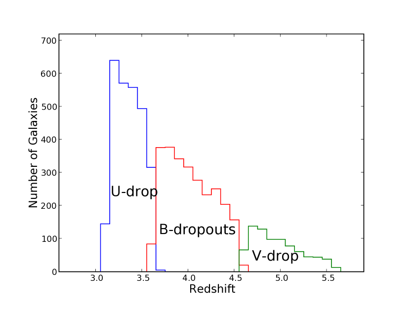
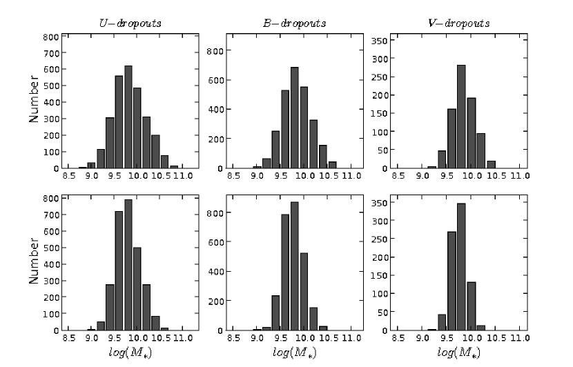
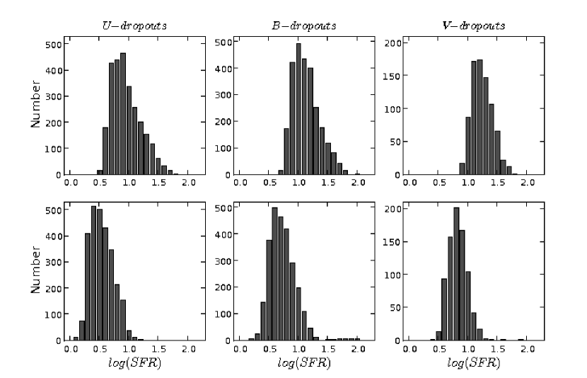
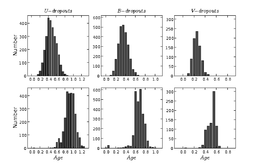
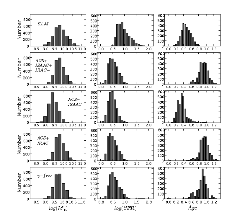
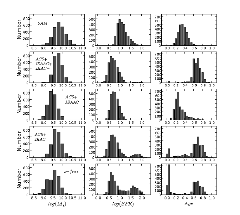
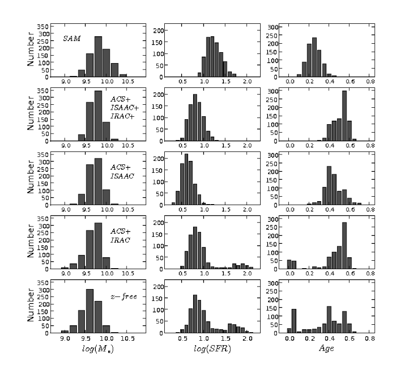
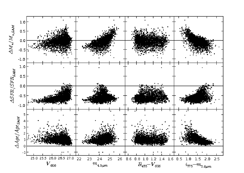
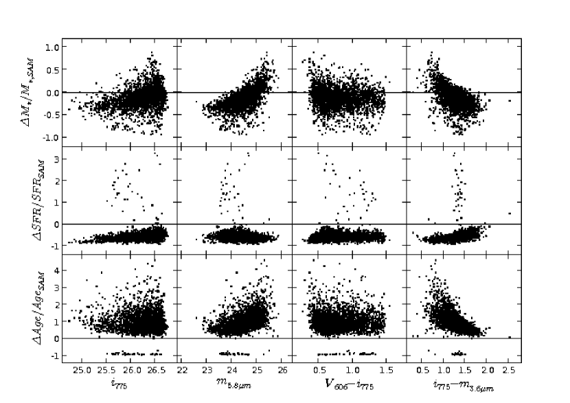
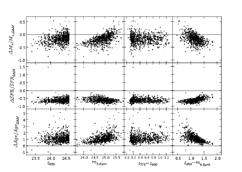
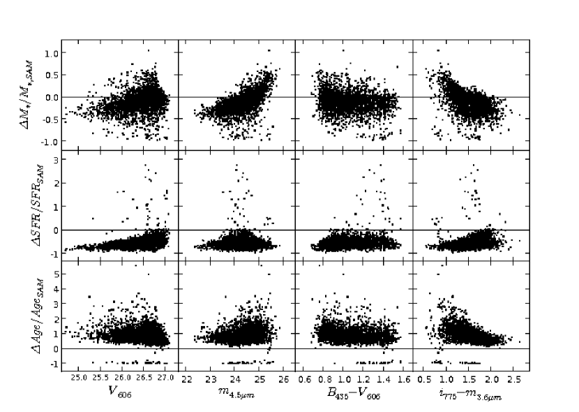
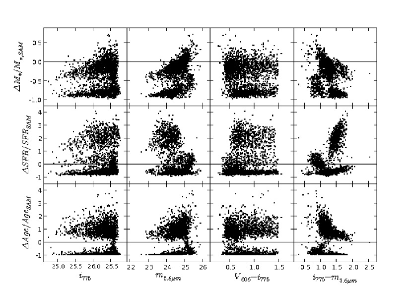
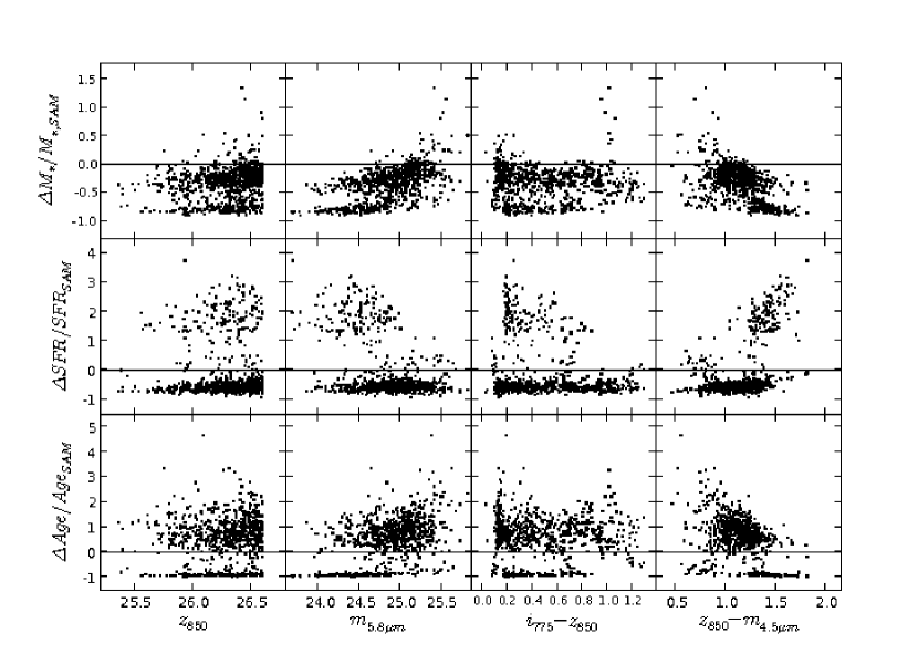
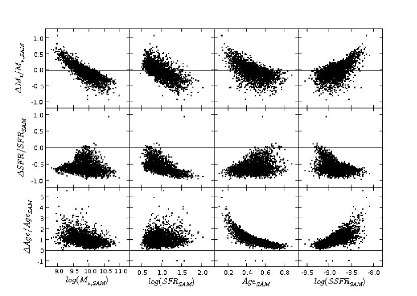
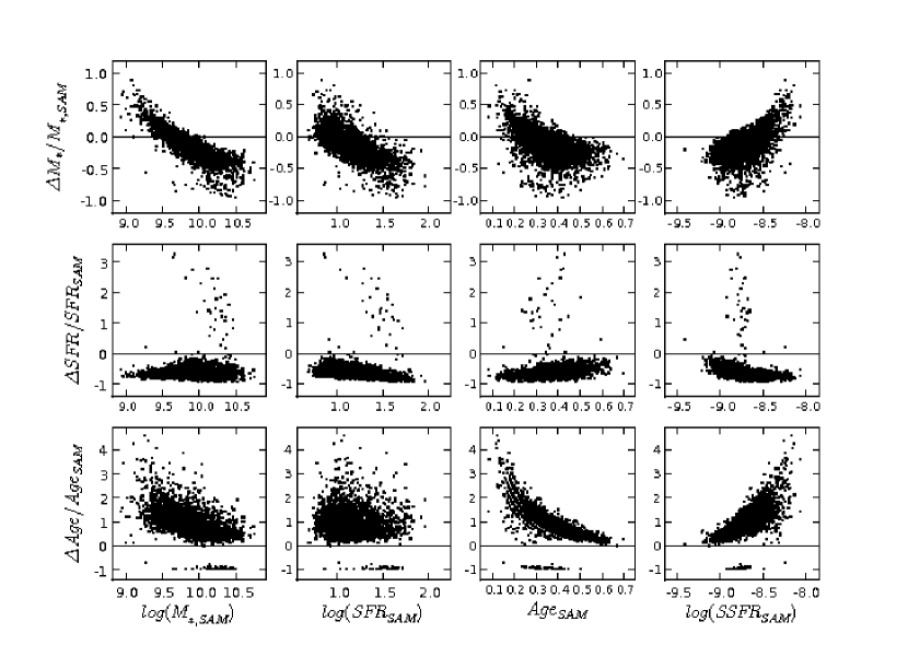
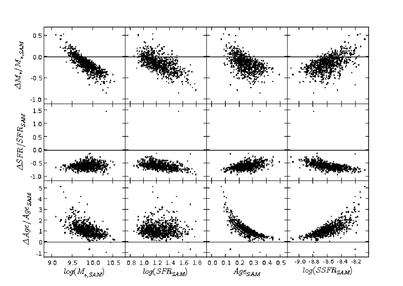
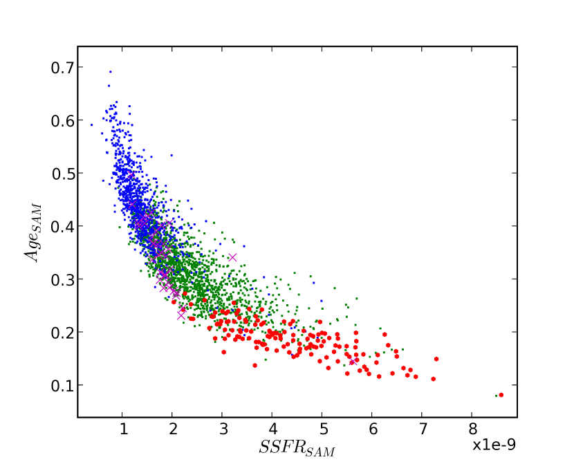
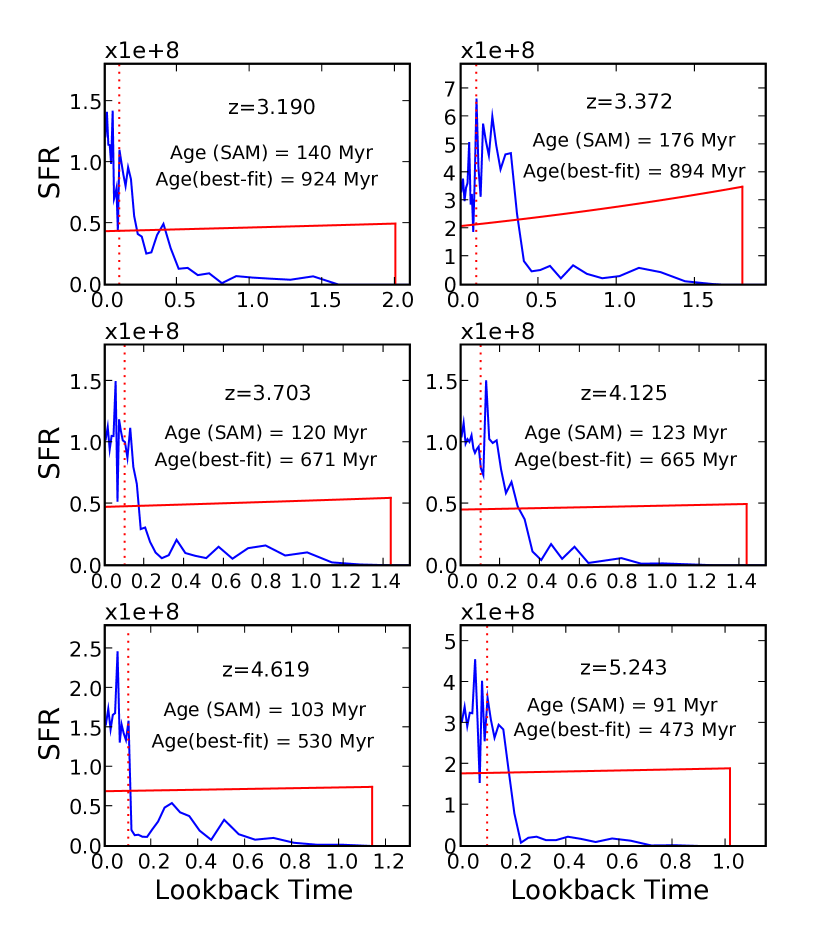
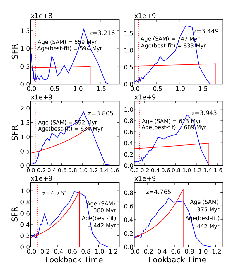
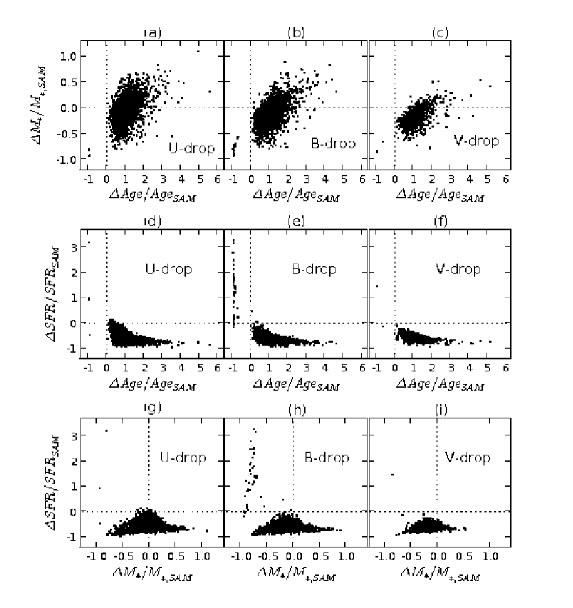
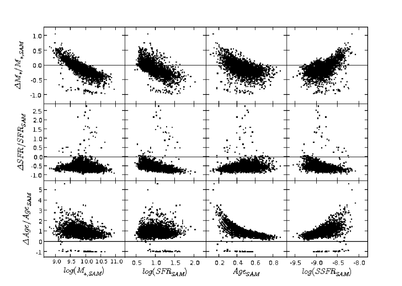
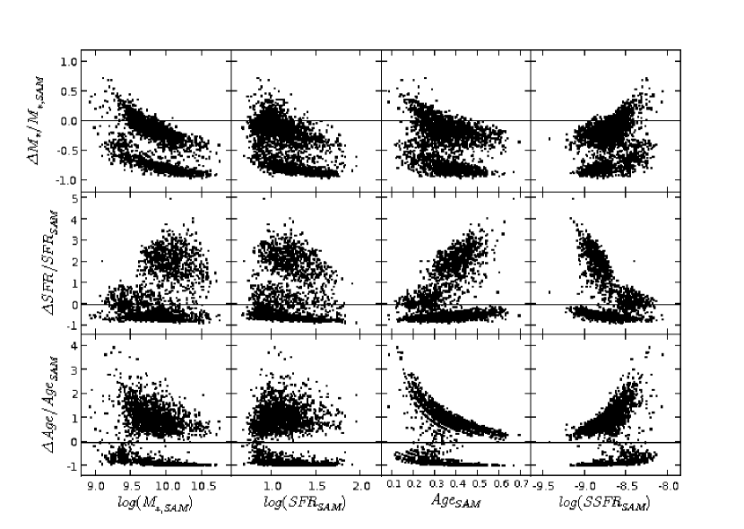
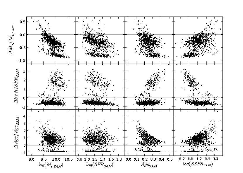
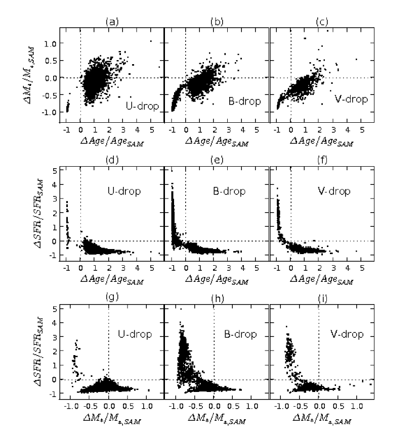
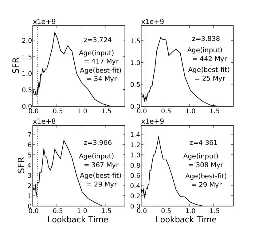
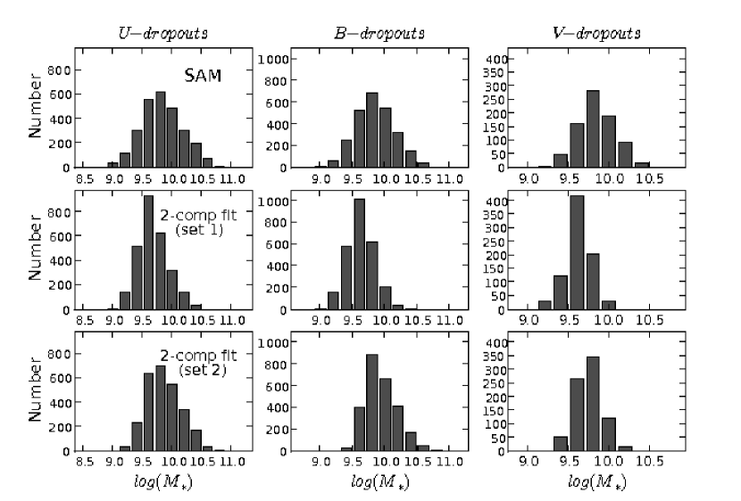
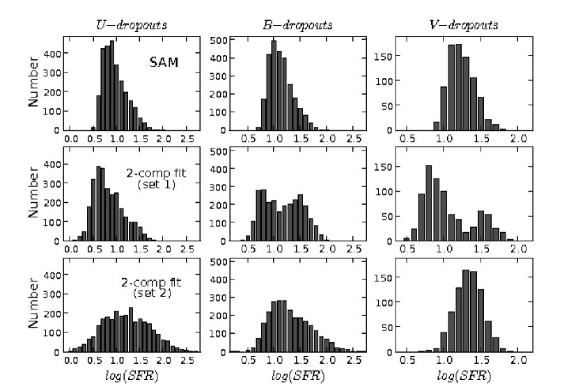
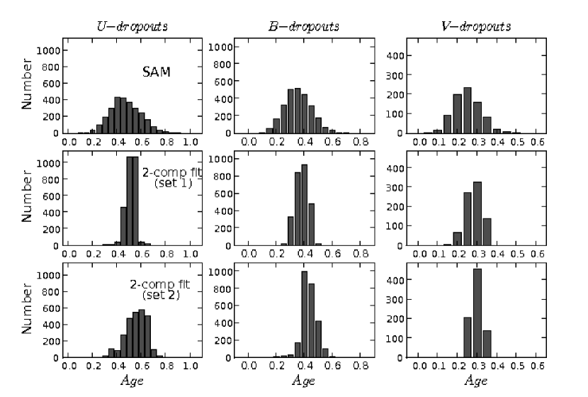
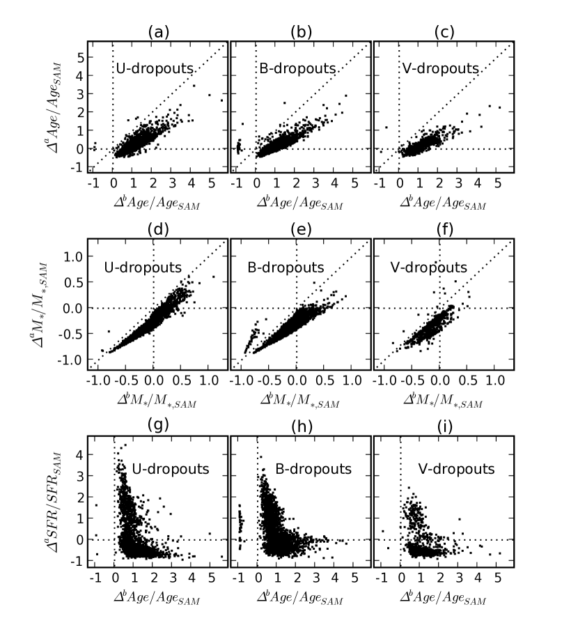
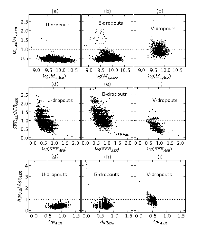
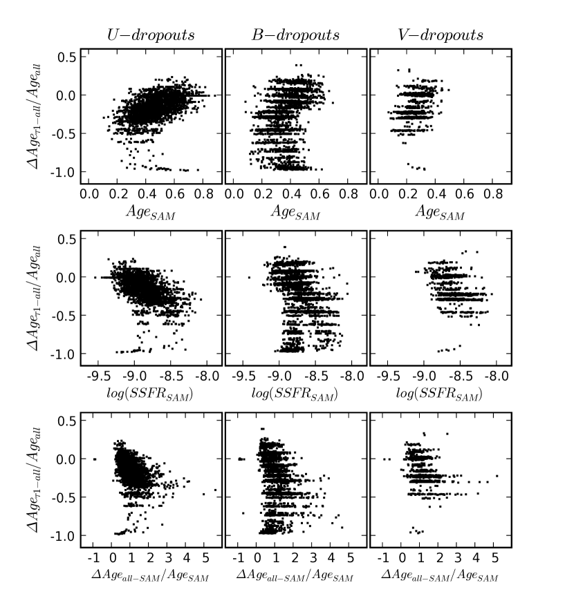
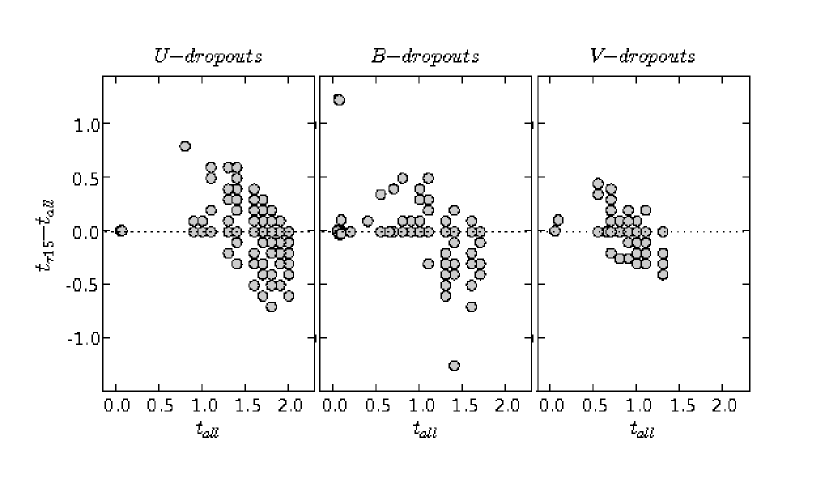
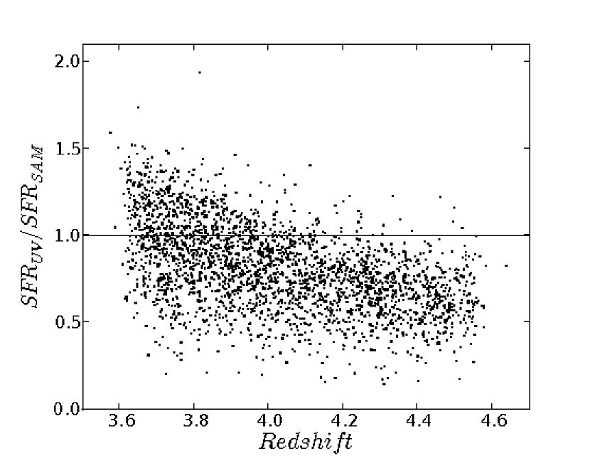
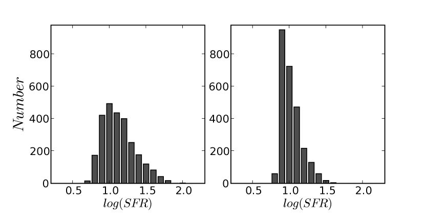
IMF	$\tau$ (Gyr)	$t$ (Gyr)	metallicity ($Z_{\sun}$)	internal extinction	IGM extinction
Chabrier	0.2-15.0	0.01-2.3	0.2, 0.4, 1.0	Calzetti	Madau

Table 2: Mean Values of Stellar Population Parameter Distributions

	Redshift	Stellar Mass ($M_{\sun}$)	SFR ($M_{\sun}$/yr)	Mean Age (Gyr)
U-dropouts
SAMs	3.36	9.376$\times 10^{9}$	11.005	0.465
$SED_{z-fix}$	3.36	7.594$\times 10^{9}$	3.887	0.915
$SED_{z-free}$	3.27	7.038$\times 10^{9}$	4.682	0.870
B-dropouts
SAMs	4.02	8.888$\times 10^{9}$	15.650	0.353
$SED_{z-fix}$	4.02	6.680$\times 10^{9}$	6.638	0.667
$SED_{z-free}$	3.88	4.327$\times 10^{9}$	19.891	0.420
V-dropouts
SAMs	4.97	7.946$\times 10^{9}$	18.920	0.249
$SED_{z-fix}$	4.97	5.983$\times 10^{9}$	7.287	0.508
$SED_{z-free}$	4.88	4.496$\times 10^{9}$	16.905	0.344

Table 3: Means and Standard Deviations of Relative Offsets for various Stellar Population Parameters

	Redshift	Stellar Mass	SFR	Mean Age
U-dropouts
$SED_{z-fix}$	$\cdots$	-0.039$\pm$0.232	-0.585$\pm$0.185	1.075$\pm$0.510
$SED_{z-free}$	-0.021$\pm$0.015	-0.108$\pm$0.230	-0.530$\pm$0.258	0.955$\pm$0.502
B-dropouts
$SED_{z-fix}$	$\cdots$	-0.120$\pm$0.228	-0.558$\pm$0.288	1.009$\pm$0.586
$SED_{z-free}$	-0.030$\pm$0.031	-0.371$\pm$0.355	0.212$\pm$1.181	0.273$\pm$1.012
V-dropouts
$SED_{z-fix}$	$\cdots$	-0.169$\pm$0.179	-0.597$\pm$0.133	1.162$\pm$0.589
$SED_{z-free}$	-0.014$\pm$0.012	-0.339$\pm$0.274	-0.094$\pm$0.964	0.487$\pm$0.875

Table 4: Relative Changes of the Mean Stellar Masses and Ages with the Limited $\tau$ Range

$\tau$s Used for Fitting	Stellar Mass ($\%$)	Mean Age ($\%$)
U-dropouts
$\tau\leq 1.0$ Gyr	-4.9	-15
$\tau=15.0$ Gyr	-8.0	-12
B-dropouts
$\tau\leq 1.0$ Gyr	-12	-26
$\tau=15.0$ Gyr	-3.4	-7.4
V-dropouts
$\tau\leq 1.0$ Gyr	-5.4	-16
$\tau=15.0$ Gyr	-3.2	-6.6

Table 5: Toy Models

	Model 1	Model 2	Model 3
input
$\tau$ (Gyr)	15.0	0.2	0.2 (young), 0.2 (old)
$t$ (Gyr)	0.01, 0.05, 0.1, 0.5, 1.0	0.1, 0.2, 0.5, 1.0, 1.3	0.1 (young), 1.0 (old)
$E(B-V)$	0, 0.05, 0.1, 0.2	0, 0.05, 0.1, 0.2	0.0, 0.2
Mass Fraction	$\cdots$	$\cdots$	0.1, 0.26, 0.52, 1.0, 2.6
Number of SEDs	120	120	60
used for fitting
$\tau$ (Gyr)	$\leq 1.0$	$\geq 8.0$	$0.2\leq\tau\leq 15.0$
$t$ (Gyr)	0.01 - 2.3	0.01 - 2.3	0.01 - 2.3

References

- Adelberger et al. (1998) Adelberger, K. L., Steidel, C. C., Giavalisco, M., Dickinson, M., Pettini, M., & Kellogg, M. 1998, ApJ, 505, 18
- Ando et al. (2004) Ando, M., Ohta, K., Iwata, I., Watanabe, C., Tamura, N., Akiyama, M., & Aoki, K. 2004, ApJ, 610,635
- Bruzual & Charlot (2003) Bruzual, G. & Charlot, S. 2003, MNRAS, 344, 1000
- Calzetti et al. (2000) Calzetti, D., Armus, L., Bohlin, R. C., Kinney, A. L., Koornneef, J., & Storchi-Bergmann, T. 2000, ApJ, 533, 682
- Chabrier (2003) Chabrier, G. 2003, PASP, 115, 763
- Drory et al. (2005) Drory, N., Salvato, M., Gabasch, A., Bender, R., Hopp, U., Feulner, G., & Pannella, M. 2005, ApJ, 619, L131
- Dye et al. (2008) Dye, S. et al. 2008, MNRAS, 386, 1107
- Elsner et al. (2008) Elsner, F., Feulner, G., & Hopp, U. 2008, A&A, 477, 503
- Finkelstein et al. (2008) Finkelstein, S. L., Rhoads, J. E., Malhotra, S., & Grogin, N. 2008, ApJ, in press (arXiv.0806.3269)
- Finkelstein et al. (2007) Finkelstein, S. L., Rhoads, J. E., Malhotra, S., Pirzkal, N., & Wang, J. 2007, ApJ, 660, 1023
- Finlator et al. (2007) Finlator, K., Dav, R. & Oppenheimer, B. D. 2007, MNRAS, 376, 1861
- Giavalisco (2002) Giavalisco, M. 2002, ARA&A, 40, 579
- Giavalisco et al. (2004a) Giavalisco, M. et al. 2004a, ApJ, 600, L93
- Giavalisco et al. (2004b) Giavalisco, M. et al. 2004b, ApJ, 600, L103
- Hopkins et al. (2001) Hopkins, A. M., Connolly, A. J., Haarsma, D. B. & Cram, L. E. 2001, AJ, 122, 288
- Idzi (2007) Idzi, R. 2007, Ph.D Thesis, Johns Hopkins University
- Idzi et al. (2004) Idzi, R., Somerville, R., Papovich, C., Ferguson, H. C., Giavalisco, M., Kretchmer, C., & Lotz, J. 2004, ApJ, 600, L115
- Kauffmann et al. (2003) Kauffmann, G. et al. 2003, MNRAS, 341, 33
- Kennicutt (1998) Kennicutt, R. C. Jr. 1998, ARA&A, 36, 189
- Labb et al. (2005) Labb, I. et al. 2005, ApJ, 624, L81
- Lai et al. (2007) Lai, K., Huang, J.-S., Fazio, G., Cowie, L. L., Hu, E. M., & Kakazu, Y. 2007, ApJ, 655, 704
- Lee et al. (2006) Lee, K.-S., Giavalisco, M., Gnedin, O. Y., Somerville, R. S., Ferguson, H. C., Dickinson, M., & Ouchi, M. 2006, ApJ, 642, 63
- Lowenthal et al. (1997) Lowenthal, J. D. et al. 1997, ApJ, 481, 673
- Madau (1995) Madau, P. 1995, ApJ, 441, 18
- Madau et al. (1996) Madau, P., Ferguson, H. C, Dickinson, M. E., Giavalisco, M., Steidel, C. C., & Fruchter, A. 1996, MNRAS, 283, 1388
- Nagamine et al. (2005) Nagamine, K., Cen, R., Hernquist, L., Ostriker, J. P., & Springel, V. 2005, ApJ, 618, 23
- Night et al. (2006) Night, C., Nagamine, K., Springel, V., & Hernquist, L. 2006, MNRAS, 366, 705
- Oke (1974) Oke, J. B. 1974, ApJS, 27, 21
- Papovich et al. (2001) Papovich, C., Dickinson, M., & Ferguson, H. C. 2001, ApJ, 559, 620
- Papovich et al. (2005) Papovich, C., Dickinson, M., Giavalisco, M., Conselice, C. J., & Ferguson, H. C. 2005, ApJ, 631, 101
- Papovich et al. (2004) Papovich, C. et al. 2004, ApJ, 600, L111
- Pettini et al. (2001) Pettini, M., Shapley, A. E., Steidel, C. C., Cuby, J.-G., Dickinson, M., Moorwood, A. F. M., Adelberger, K. L., & Giavalisco, M. 2001, ApJ, 554, 981
- Pozzetti et al. (2007) Pozzetti, L. et al. 2007, A&A, 474, 443
- Ravindranath et al. (2006) Ravindranath, S. et al. 2006, ApJ, 652, 963
- Rhoads et al. (2008) Rhoads, J. E. et al. 2008, ApJ, submitted (arXiv.0805.1056)
- Salpeter (1955) Salpeter, E. E. 1955, ApJ, 121, 161
- Sawicki & Thompson (2006) Sawicki, M., & Thompson, D. 2006, ApJ, 648, 299
- Sawicki & Yee (1998) Sawicki, M. & Yee, H. K. C. 1998, AJ, 115, 1329
- Scoville et al. (2007) Scoville, N. Z. et al. 2007, ApJS, 172, 1
- Shapley et al. (2001) Shapley, A. E., Steidel, C. C., Adelberger, K. L., Dickinson, M., Giavalisco, M., & Pettini, M. 2001, ApJ, 562, 95
- Shapley et al. (2005) Shapley, A. E., Steidel, C. C., Erb, D. K., Reddy, N. A., Adelberger, K. L., Pettini, M., Barmby, P., & Huang, J. 2005, ApJ, 626, 698
- Shapley et al. (2003) Shapley, A. E., Steidel, C. C., Pettini, M., & Adelberger, K. L. 2003, ApJ, 588, 65
- Shim et al. (2007) Shim, H., Im, M., Choi, P., Yan, L., & Storrie-Lombardi, L. 2007, ApJ, 669, 749
- Somerville et al. (2008) Somerville, R. S., Hopkins, P. F., Cox, T. J., Robertson, B. E., & Hernquist, L. 2008, MNRAS, in press (arXiv.0808.1227)
- Somerville & Kolatt (1999) Somerville, R. S. & Kolatt, T. S. 1999, MNRAS, 305, 1
- Somerville & Primack (1999) Somerville, R. S. & Primack, J. R. 1999, MNRAS, 310, 1087
- Somerville et al. (2001) Somerville, R. S., Primack, J. R., & Faber, S. M. 2001, MNRAS, 320, 504
- Stark et al. (2007) Stark, D. P., Bunker, A. J., Ellis, R. S., Eyles, L. P., & Lacy, M. 2007, ApJ, 659, 84
- Steidel et al. (1998) Steidel, C. C., Adelberger, K. L., Dickinson, M., Giavalisco, M., Pettini, M., & Kellogg, M. 1998, ApJ, 492, 428
- Steidel et al. (1999) Steidel, C. C., Adelberger, K. L., Giavalisco, M., Dickinson, M., & Pettini, M. 1999, ApJ, 519, 1
- Steidel et al. (2003) Steidel, C. C., Adelberger, K. L., Shapley, A. E., Pettini, M., Dickinson, M., & Giavalisco, M. 2003, ApJ, 592, 728
- Steidel et al. (1996) Steidel, C. C., Giavalisco, M., Pettini, M., Dickinson, M., & Adelberger, K. L. 1996, ApJ, 462, L17
- Vanzella et al. (2006) Vanzella, E. et al. 2006, A&A, 454, 423
- Verma et al. (2007) Verma, A., Lehnert, M. D., Förster Schreiber, N. M., Natascha M., Bremer, M. N., & Douglas, L. 2007, MNRAS, 377, 1024
- Wuyts et al. (2007) Wuyts, S. et al. 2007, ApJ, 655, 51
- Yan et al. (2006) Yan, H., Dickinson, M., Giavalisco, M., Stern, D., Eisenhardt, P. R. M., & Ferguson, H. C. 2006, ApJ, 651, 24