Hydrodynamical N-body simulations of coupled dark energy cosmologies

Abstract

If the accelerated expansion of the Universe at the present epoch is driven by a dark energy scalar field, there may well be a non-trivial coupling between the dark energy and the cold dark matter (CDM) fluid. Such interactions give rise to new features in cosmological structure growth, like an additional long-range attractive force between CDM particles, or variations of the dark matter particle mass with time. We have implemented these effects in the N-body code GADGET-2 and present results of a series of high-resolution N-body simulations where the dark energy component is directly interacting with the cold dark matter. As a consequence of the new physics, CDM and baryon distributions evolve differently both in the linear and in the nonlinear regime of structure formation. Already on large scales a linear bias develops between these two components, which is further enhanced by the nonlinear evolution. We also find, in contrast with previous work, that the density profiles of CDM halos are less concentrated in coupled dark energy cosmologies compared with $\Lambda$CDM, and that this feature does not depend on the initial conditions setup, but is a specific consequence of the extra physics induced by the coupling. Also, the baryon fraction in halos in the coupled models is significantly reduced below the universal baryon fraction. These features alleviate tensions between observations and the $\Lambda$CDM model on small scales. Our methodology is ideally suited to explore the predictions of coupled dark energy models in the fully non-linear regime, which can provide powerful constraints for the viable parameter space of such scenarios.

1 Introduction

The last decade has seen an astonishing amount of new cosmological data from many different experiments, ranging from large-scale structure surveys (Percival et al., 2001, e.g.) to Cosmic Microwave Background (CMB) (Komatsu et al., 2008) and Type Ia Supernovae (Riess et al., 1998; Perlmutter et al., 1999; Astier et al., 2006) observations. These experiments all consistently show that the Universe is almost spatially flat with a current expansion rate of about $70\,{\rm km\,s^{-1}Mpc^{-1}}$, and contains a total amount of matter that accounts for only $\sim 24\%$ of the total energy density. From a theoretical point of view, understanding the remaining $76\%$ – which must be in the form of some dark energy (DE) component able to drive an accelerated expansion – is a serious challenge.

A simple cosmological constant would be in agreement with a large number of observational datasets, but would also raise two fundamental questions concerning its fine-tuned value and the coincidence of its domination over cold dark matter (CDM) only at a relatively recent cosmological epoch. An alternative consists of identifying the dark energy component with a dynamic scalar field (Wetterich, 1988; Ratra & Peebles, 1988), thereby seeking an explanation of the fundamental problems challenging the cosmological constant in the properties of the dynamic evolution of such scalar field.

An interesting suggestion recently developed concerns the investigation of possible interactions between the dark energy scalar field and other matter species in the Universe (Wetterich, 1995; Amendola, 2000; Farrar & Peebles, 2004; Gubser & Peebles, 2004; Farrar & Rosen, 2007). The existence of such a coupling could provide a unique handle for a deeper understanding of the DE problem (Quartin et al., 2008; Brookfield et al., 2008; Gromov et al., 2004; Mangano et al., 2003; Anderson & Carroll, 1997). It is then crucial to understand in detail what effects such a coupling imprints on observable features like, for example, the CMB and structure formation (La Vacca et al., 2009; Bean et al., 2008; Bertolami et al., 2007; Matarrese et al., 2003; Wang et al., 2007; Guo et al., 2007; Mainini & Bonometto, 2007a; Lee et al., 2006).

In this paper, we perform the first fully self-consistent high-resolution hydrodynamic N-body simulations of cosmic structure formation for a selected family of coupled DE cosmologies. The interaction between DE and CDM is expected to imprint characteristic features in linear and nonlinear structures, and could possibly open up new ways to overcome a series of observational challenges for the $\Lambda$CDM concordance cosmology, ranging from the satellite abundance in CDM halos (Navarro et al., 1996), to the observed low baryon fraction in large galaxy clusters (Allen et al., 2004; Vikhlinin et al., 2006; LaRoque et al., 2006), and to the so-called “cusp-core” problem for the density profiles of CDM halos, that was first raised in relation to observations of dwarf and low-surface-brightness galaxies (Moore, 1994; Flores & Primack, 1994; Simon et al., 2003), but that more recent studies seem to extend to a wider range of objects including Milky-Way type spiral galaxies (Navarro & Steinmetz, 2000; Binney & Evans, 2001) up to galaxy groups and clusters (Sand et al., 2002, 2004; Newman et al., 2009).

In the following we will consider DE as the energy associated with a scalar field $\phi$ (Wetterich, 1988; Ratra & Peebles, 1988) whose energy density and pressure are defined respectively as the $(0,0)$ and $(0,i)$ components of its stress energy tensor, so that:

$$\rho_{\phi}\equiv\frac{1}{2}\frac{{\phi^{\prime}}^{2}}{a^{2}}+U(\phi)\,,$$ (1)

$$p_{\phi}\equiv\frac{1}{2}\frac{{\phi^{\prime}}^{2}}{a^{2}}-U(\phi)\,,$$ (2)

with $U(\phi)$ being the self interaction potential. The models we investigate in this work by means of detailed high-resolution N-body simulations are physically identical to the ones already studied by Macciò et al. (2004). With respect to this previous work, however, our analysis significantly improves on the statistics of the number of cosmic structures analyzed in each of our different cosmological models and on the dynamic range of the simulations. We also extend the analysis to a wider range of observable effects arising from the new physics of the DE-CDM interaction, and we include hydrodynamics. Despite the physical models investigated be identical, our outcomes are starkly different from the ones found in Macciò et al. (2004).

This work is organized as follows. In Section 2 we detail the coupled DE cosmologies under investigation, both regarding the background evolution and the perturbations, and we introduce a numerical package to integrate the full set of background and perturbation equations up to linear order. In Section 3, we describe the numerical methods we use, and the particular set of simulations we have run. We then present and discuss our results for N-body simulations for a series of coupled DE models in Section 4. Finally, in Section 5 we draw our conclusions.

2 Coupled dark energy cosmologies

Coupled cosmologies can be described following the consideration (Kodama & Sasaki, 1984) that in any multicomponent system, though the total stress energy tensor ${T{{}^{\mu}}}_{\nu}$ is conserved

$$\sum_{\alpha}\nabla_{\nu}T^{\nu}_{(\alpha)\mu}=0\,,$$ (3)

the ${T{{}^{\mu}}}_{\nu(\alpha)}$ for each species $\alpha$ is, in general, not conserved and its divergence has a source term $Q_{(\alpha)\mu}$ representing the possibility that species are coupled:

$$\nabla_{\nu}T^{\nu}_{(\alpha)\mu}=Q_{(\alpha)\mu}\,,$$ (4)

with the constraint

$$\sum_{\alpha}Q_{(\alpha)\mu}=0~{}~{}~{}.$$ (5)

Furthermore, we will assume a flat Friedmann-Robertson-Walker (FRW) cosmology, in which the line element can be written as ${\rm d}s^{2}=a^{2}(\tau)(-{\rm d}\tau^{2}+\delta_{ij}{\rm d}x^{i}{\rm d}x^{j})$ where $a(\tau)$ is the scale factor.

2.1 Background

The Lagrangian of the system is of the form:

$${\cal L}=-\frac{1}{2}\partial^{\mu}\phi\partial_{\mu}\phi-U(\phi)-m(\phi)\bar{\psi}\psi+{\cal L}_{\rm kin}[\psi]\,,$$ (6)

in which the mass of matter fields $\psi$ coupled to the DE is a function of the scalar field $\phi$. In the following we will consider the case in which the DE is only coupled to cold dark matter (CDM, hereafter denoted with a subscript $c$). The choice $m(\phi)$ specifies the coupling and as a consequence the source term $Q_{(\phi)\mu}$ via the expression:

$$Q_{(\phi)\mu}=\frac{\partial\ln{m(\phi)}}{\partial\phi}\rho_{c}\,\partial_{\mu}\phi.$$ (7)

Due to the constraint (5), if no other species is involved in the coupling, $Q_{(c)\mu}=-Q_{(\phi)\mu}$.

The zero-component of equation (4) provides the conservation equations for the energy densities of each species:

$$\rho_{\phi}^{\prime} = -3{\cal{H}}\rho_{\phi}(1+w_{\phi})-Q_{(\phi)0}\,\,\,\,,$$ (8)

$$\rho_{c}^{\prime} = -3{\cal{H}}\rho_{c}+Q_{(\phi)0}~{}~{}~{}.$$

Here we have treated each component as a fluid with ${T^{\nu}}_{(\alpha)\mu}=(\rho_{\alpha}+p_{\alpha})u_{\mu}u^{\nu}+p_{\alpha}\delta^{\nu}_{\mu}$, where $u_{\mu}=(-a,0,0,0)$ is the fluid 4-velocity and $w_{\alpha}\equiv p_{\alpha}/\rho_{\alpha}$ is the equation of state. The class of models considered here corresponds to the choice:

$$m(\phi)=m_{0}e^{-\beta(\phi)\frac{\phi}{M}}\,,$$ (9)

with the coupling term equal to

$$Q_{(\phi)0}=-\frac{\beta(\phi)}{M}\rho_{c}\phi^{\prime}\,.$$ (10)

This set of cosmologies has been widely investigated, for $\beta(\phi)$ given by a constant, both in its background and linear perturbation features (Wetterich, 1995; Amendola, 2000) as well as with regard to the effects on structure formation (Amendola, 2004; Pettorino & Baccigalupi, 2008) , and via a first N-body simulation (Macciò et al., 2004).

2.2 Linear perturbations

We now perturb the quantities involved in our cosmological framework up to the first order in the perturbations (Kodama & Sasaki, 1984; Ma & Bertschinger, 1995). The perturbed metric tensor can then be written as

$$\tilde{g}_{\mu\nu}(\tau,\bf{x})=g_{\mu\nu}(\tau)+\delta g_{\mu\nu}(\tau,\bf{x})\,,$$ (11)

where $\delta g_{\mu\nu}\ll 1$ is the linear metric perturbation, whose expression in Fourier space is given by:

$$\delta g_{00}=-2a^{2}AY\ \ ,\ \ \delta g_{0i}=-a^{2}BY_{i}\ \,,$$

$$\ \ \delta g_{ij}=2a^{2}[H_{L}Y\delta_{ij}+H_{T}Y_{ij}] \,,$$ (12)

where $A,B,H_{L},H_{T}$ are functions of time and of the wave vector $\bf{k}$, and $Y_{i},Y_{ij}$ are the vector and tensor harmonic functions obtained by deriving Y, defined as the solution of the Laplace equation $\delta^{ij}\nabla_{i}\nabla_{j}Y=-|k|^{2}Y$. Analogously, the perturbed stress energy tensor for each fluid $(\alpha)$ can be written as $\tilde{T}^{\mu}_{(\alpha)\nu}=T^{\mu}_{(\alpha)\nu}+\delta T^{\mu}_{(\alpha)\nu}$ where the perturbations read as:

$$\delta T^{0}_{(\alpha)0} =-\rho_{(\alpha)}\delta_{(\alpha)}Y\,,$$

$$\delta T^{0}_{(\alpha)i} =h_{(\alpha)}(v_{(\alpha)}-B)Y_{i}\,,$$

$$\delta T^{i}_{(\alpha)0} =-h_{(\alpha)}v_{(\alpha)}Y^{i}\,,$$

$$\delta T^{i}_{(\alpha)j} =p_{(\alpha)}\left[\pi_{L(\alpha)}Y\delta^{i}_{j}+\pi_{T(\alpha)}Y^{i}_{j}\right]\,.$$

The perturbed conservation equations then become:

$$(\rho_{\alpha}\delta_{\alpha})^{\prime}+3{\cal H}\rho_{\alpha}\delta_{\alpha}+h_{\alpha}(kv_{\alpha}+3H^{\prime}_{L})+3{\cal H}p_{\alpha}\pi_{L\alpha}=-\delta Q_{(\alpha)0}$$ (14)

for the energy density perturbation $\delta_{\alpha}=\delta\rho_{\alpha}/\rho_{\alpha}$, and:

$$\left[h_{\alpha}(v_{\alpha}-B)\right]^{\prime}+4{\cal H}h_{\alpha}(v_{\alpha}-B)$$

$$-kp_{\alpha}\pi_{L\alpha}-h_{\alpha}kA+\frac{2}{3}kp\pi_{T\alpha}=\delta Q_{(\alpha)i}$$ (15)

for the velocity perturbation $v_{\alpha}$.

The scalar field $\phi$ can also be perturbed, yielding in Fourier space

$$\tilde{\phi}=\phi+\delta\phi=\phi+\chi(\tau)Y\,.$$ (16)

Furthermore, we can express the perturbations of the source as:

$$\delta Q_{(\phi)0}=-\frac{\beta(\phi)}{M}\rho_{c}\delta\phi^{\prime}-\frac{\beta(\phi)}{M}\phi^{\prime}\delta\rho_{c}-\frac{\beta_{,\phi}}{M}\phi^{\prime}\rho_{c}\delta\phi\,,$$ (17)

$$\delta Q_{(\phi)i}=k\frac{\beta(\phi)}{M}\rho_{c}\delta\phi\,.$$ (18)

In the Newtonian gauge $(B=0,H_{T}=0,H_{L}={\bf{\Phi}},A=\bf{\Psi})$ the set of equations for the density and velocity perturbations for DE and CDM read:

$$\delta\rho_{\phi}^{\prime}+3{\cal H}(\delta\rho_{\phi}+\delta p_{\phi})+kh_{\phi}v_{\phi}+3h_{\phi}{\bf{\Phi}}^{\prime}=$$ (19)

$$\frac{\beta(\phi)}{M}\rho_{c}\delta\phi^{\prime}+\frac{\beta(\phi)}{M}\phi^{\prime}\delta\rho_{c}+\frac{\beta_{,\phi}}{M}\phi^{\prime}\delta\phi\rho_{c}\,,$$

$$\delta\rho_{c}^{\prime}+3{\cal H}\delta\rho_{c}+k\rho_{c}v_{c}+3\rho_{c}{\bf{\Phi}}^{\prime}=$$

$$-\frac{\beta(\phi)}{M}\rho_{c}\delta\phi^{\prime}-\frac{\beta(\phi)}{M}\phi^{\prime}\delta\rho_{c}-\frac{\beta_{,\phi}}{M}\phi^{\prime}\delta\phi\rho_{c}\,,$$

$$h_{\phi}v_{\phi}^{\prime}+\left(h_{\phi}^{\prime}+4{\cal H}h_{\phi}\right)v_{\phi}-k\delta p_{\phi}-kh_{\phi}{\bf{\Psi}}=k\frac{\beta(\phi)}{M}\rho_{c}\delta\phi\,,$$

$$v_{c}^{\prime}+\left({\cal H}-\frac{\beta(\phi)}{M}\phi^{\prime}\right)v_{c}-k{\bf{\Psi}}=-k\frac{\beta(\phi)}{M}\delta\phi\,.$$

The perturbed Klein Gordon equation in Newtonian gauge reads:

$$\delta\phi^{\prime\prime}+2{\cal H}\delta\phi^{\prime}+\left(k^{2}+a^{2}U_{,\phi\phi}\right)\delta\phi-\phi^{\prime}\left({\bf{\Psi}}^{\prime}-3{\bf{\Phi}^{\prime}}\right) +$$

$$2a^{2}U_{,\phi}{\bf{\Psi}}=3{\cal H}^{2}\Omega_{c}\left[\beta(\phi)\delta_{c}+2\beta(\phi){\bf{\Psi}}+\beta_{,\phi}(\phi)\delta\phi\right] \,.$$ (20)

For the N-body implementation we are interested in, the Newtonian limit holds, for which $\lambda\equiv{\cal H}/k\ll 1$. In this case we have

$$\delta\phi\sim 3\lambda^{2}\Omega_{c}\beta(\phi)\delta_{c}\,.$$ (21)

In this limit, the gravitational potential is approximately given by

$${\bf{\Phi}}\sim\frac{3}{2}\frac{\lambda^{2}}{M^{2}}\sum_{\alpha\neq\phi}\Omega_{\alpha}\delta_{\alpha}\,.$$ (22)

We can then define an effective gravitational potential

$${\bf{\Phi_{c}}}\equiv{\bf{\Phi}}+\frac{\beta(\phi)}{M}\delta\phi,$$ (23)

which also reads, in real space and after substituting the expressions for ${\bf{\Phi}}$ (Eqn. 22) and for $\delta\phi$ (Eqn. 21):

$$\nabla^{2}{\bf{\Phi_{c}}}=-\frac{a^{2}}{2}\rho_{c}\delta_{c}\left(1+2\beta^{2}(\phi)\right)-\frac{a^{2}}{2}\sum_{\alpha\neq\phi,c}\rho_{\alpha}\delta_{\alpha}\,,$$ (24)

where the last term takes into account the case in which other components not coupled to the DE are present in the total energy budget of the Universe. Cold dark matter then feels an effective gravitational constant

$$\tilde{G}_{c}=G_{N}[1+2\beta^{2}(\phi)],$$ (25)

where $G_{N}$ is the usual Newtonian value. Therefore, the strength of the gravitational interaction is not a constant anymore if $\beta$ is a function of the scalar field $\phi$. The last equation in (19), written in real space and in terms of the effective gravitational potential, gives a modified Euler equation of the form:

$${\mn@boldsymbol{\nabla}}{\mn@boldsymbol{v}}_{c}^{\prime}+\left({\cal H}-\frac{\beta(\phi)}{M}\phi^{\prime}\right){\mn@boldsymbol{\nabla}}{\mn@boldsymbol{v}}_{c}+$$

$$\frac{3}{2}{\cal H}^{2}\left[\Omega_{c}\delta_{c}+2\Omega_{c}\delta_{c}\beta^{2}(\phi)+\sum_{\alpha\neq\phi,c}\Omega_{\alpha}\delta_{\alpha}\right]=0\,.$$ (26)

As in Amendola (2004), if we assume that the CDM is concentrated in one particle of mass $m_{c}$ at a distance $r$ from a particle of mass $M_{c}$ at the origin, we can rewrite the CDM density contribution as

$$\Omega_{c}\delta_{c}=\frac{8\pi GM_{c}e^{-\int{\beta(\phi){\rm d}\phi}}{\delta}(0)}{3{\cal H}^{2}a}\ ,$$ (27)

where we have used the fact that a non-relativistic particle at position ${\mn@boldsymbol{r}}$ has a density given by $m_{c}n{\delta({\mn@boldsymbol{r}})}$ (where ${\delta({\mn@boldsymbol{r}})}$ stands for the Dirac distribution) with mass given by $m_{c}\propto e^{-\int{\beta(\phi){\rm d}\phi}}$, formally obtained from equation (2.1). We have further assumed that the density of the $M_{c}$ mass particle is much larger than $\rho_{c}$. The Euler equation in cosmic time (${\rm d}t=a\,{\rm d}\tau$) can then be rewritten in the form of an acceleration equation for the particle at position ${\mn@boldsymbol{r}}$:

$$\dot{{\mn@boldsymbol{v}}}_{c}=-\tilde{H}{\mn@boldsymbol{v}}_{c}-{\mn@boldsymbol{\nabla}}\frac{\tilde{G}_{c}\tilde{M}_{c}}{r}\,,$$ (28)

where we explicitely see that the usual equation is modified in three ways.

First, the velocity-dependent term now contains an additional contribution given by the second term of the expression defining $\tilde{H}$:

$$\tilde{H}\equiv H\left(1-\frac{\beta(\phi)}{M}\frac{\dot{\phi}}{H}\right)\ .$$ (29)

Second, the CDM particles feel an effective gravitational constant $\tilde{G}$ given by (25). Third, the CDM particles have an effective mass, varying with time, given by:

$$\tilde{M}_{c}\equiv M_{c}e^{-\int{\beta(\phi)\frac{{\rm d}\phi}{{\rm d}a}{\rm d}a}}~{}~{}~{}.$$ (30)

Eqn. 28 is very important for our discussion since it represents the starting point for the implementation of coupled DE models in an N-body code. We will discuss in detail how this implementation is realized in Sec. 3.1, but it is important to stress here that Eqn. 28 is written in a form that explicitely highlights its vectorial nature, which has not been presented in previous literature. The vectorial nature of Eqn. 28 is a key point in its numerical implementation and therefore needs to be properly taken into account.

In the N-body analysis carried out in the present paper, we consider $\beta$ to be a constant, so that the effective mass formally reads $\tilde{M}_{c}\equiv M_{c}e^{-\beta\left(\phi-\phi_{0}\right)}$. We defer an investigation of variable $\beta(\phi)$ to future work. We have numerically solved the full background and linear perturbation equations with a suitably modified version of CMBEASY (Doran, 2005), briefly described in the following section.

2.3 Background and linear perturbation integration of coupled DE models: a modified CMBEASY package

We have implemented the full background and linear perturbation equations derived in the previous section in the Boltzmann code CMBEASY (Doran, 2005) for the general case of a DE component coupled to dark matter via a coupling term given by Eqn. (4). The form of this coupling, as well as the evolution of the DE (either modelled as a scalar field or purely as a DE fluid), can be freely specified in our implementation.

Compared to the standard case of uncoupled DE, the modifications include a modified behaviour of the background evolution of CDM and DE given by Eqs. (8) and (2.1), as well as the implementation of the linear perturbations described by Eqn. (19), and their corresponding adiabatic initial conditions. The presence of a CDM-DE coupling furthermore complicates the choice of suitable initial conditions even for the background quantities, since dark matter no longer scales as $a^{-3}$, and so cannot simply be rescaled from its desired value today. For each of the models considered here, we choose to set the initial value of the scalar field close to its tracker value in the uncoupled case, and then adjust the value of the potential constant $\Lambda$ (see Eqn. (31) below) and the initial CDM energy density such that we obtain the desired present-day values.

3 The simulations

The aim of this work is to investigate the effects that a coupling between DE and other cosmological components, as introduced in Sec. 2, can have on cosmic structure formation, with a particular focus on the nonlinear regime which is not readily accessible by the linear analytic approach described in Sec. 2.2. To this end we study a set of cosmological N-body simulations performed with the code GADGET-2 (Springel, 2005), that we suitably modified for this purpose.

The required modifications of the standard algorithms of the N-body code for simulating coupled DE cosmologies are extensively described in Sec. 3.1. Interestingly, they require to reconsider and in part drop several assumptions and approximations that are usually adopted in N-body simulations. We note that previous attempts to use cosmological N-body simulations for different flavours of modified Newtonian gravity have been discussed, for example, in Macciò et al. (2004); Nusser et al. (2005); Stabenau & Jain (2006); Kesden & Kamionkowski (2006); Springel & Farrar (2007); Laszlo & Bean (2008); Sutter & Ricker (2008); Oyaizu (2008); Keselman et al. (2009) but to our knowledge Macciò et al. (2004) is the only work to date focusing on the properties of nonlinear structures in models of coupled quintessence.

Therefore, with our modified version of GADGET-2 we first ran a set of low-resolution cosmological simulations ($L_{\rm box}=320h^{-1}{\rm Mpc}$, $N_{\rm part}=2\times 128^{3}$) for the same coupled DE models investigated in Macciò et al. (2004), but with cosmological parameters updated to the latest results from WMAP (Komatsu et al., 2008) for a $\Lambda$CDM cosmological model. In the coupled models we consider, the role of DE is played by a quintessence scalar field with a Ratra-Peebles (Ratra & Peebles, 1988) self-interaction potential of the form:

$$U(\phi)=\frac{\Lambda^{4+\alpha}}{\phi^{\alpha}}\,,$$ (31)

where $\Lambda$ and $\alpha$ fix the DE scale in agreement with observations, and with a constant coupling to CDM particles only, as described in Sec. 2.1; we label them as RP1-RP6 in analogy with Macciò et al. (2004).

For four of these models ($\Lambda$CDM, RP1, RP2, RP5) we then ran high-resolution simulations in a smaller cosmological box ($L_{\rm box}=80h^{-1}$ Mpc, $N_{\rm part}=2\times 512^{3}$), and we investigated the properties of collapsed objects for this set of simulations. In addition to these four high-resolution simulations we ran other three simulations with the same resolution ($\Lambda$CDM-NO-SPH, RP5-NO-SPH, RP5-NO-GF), whose features will be described below. The cosmological parameters for our models are listed in Table 1, and the physical parameters of each model together with the details of the corresponding N-body simulations are listed in Table 2.

Parameter	Value
$\Omega_{\rm CDM}$	0.213
$H_{0}$	71.9 km s-1 Mpc-1
$\Omega_{\rm DE}$	0.743
$\sigma_{8}$	0.769
$\Omega_{b}$	0.044
$n$	0.963

Table 1: Cosmological parameters for our set of N-body simulations, consistent with the WMAP 5 year results for a $\Lambda$CDM cosmology (Komatsu et al., 2008).

Model	$\alpha$	$\beta_{b}$	$\beta_{c}$	Box Size ($h^{-1}$ Mpc)	Number of particles	$M_{b}$ ($h^{-1}M_{\odot}$)	$M_{\rm CDM}$ ($h^{-1}M_{\odot}$)	$\epsilon_{s}$ ($h^{-1}$ kpc)
$\Lambda$CDM (low)	0	0	0	320	2 $\times$ 1283	1.9 $\times$ 1011	9.2 $\times$ 1011	50.0
$\Lambda$CDM (high)	0	0	0	80	2 $\times$ 5123	4.7 $\times$ 107	2.3 $\times$ 108	3.5
$\Lambda$CDM (high - no SPH)	0	0	0	80	2 $\times$ 5123	4.7 $\times$ 107	2.3 $\times$ 108	3.5
RP1 (low)	0.143	0	0.04	320	2 $\times$ 1283	1.9 $\times$ 1011	9.2 $\times$ 1011	50.0
RP1 (high)	0.143	0	0.04	80	2 $\times$ 5123	4.7 $\times$ 107	2.3 $\times$ 108	3.5
RP2 (low)	0.143	0	0.08	320	2 $\times$ 1283	1.9 $\times$ 1011	9.2 $\times$ 1011	50.0
RP2 (high)	0.143	0	0.08	80	2 $\times$ 5123	4.7 $\times$ 107	2.3 $\times$ 108	3.5
RP3 (low)	0.143	0	0.12	320	2 $\times$ 1283	1.9 $\times$ 1011	9.2 $\times$ 1011	50.0
RP4 (low)	0.143	0	0.16	320	2 $\times$ 1283	1.9 $\times$ 1011	9.2 $\times$ 1011	50.0
RP5 (low)	0.143	0	0.2	320	2 $\times$ 1283	1.9 $\times$ 1011	9.2 $\times$ 1011	50.0
RP5 (high)	0.143	0	0.2	80	2 $\times$ 5123	4.7 $\times$ 107	2.3 $\times$ 108	3.5
RP5 (high - no SPH)	0.143	0	0.2	80	2 $\times$ 5123	4.7 $\times$ 107	2.3 $\times$ 108	3.5
RP5 (high - no GF)	0.143	0	0.2	80	2 $\times$ 5123	4.7 $\times$ 107	2.3 $\times$ 108	3.5
RP6 (low)	2.0	0	0.12	320	2 $\times$ 1283	1.9 $\times$ 1011	9.2 $\times$ 1011	50.0

Table 2: List of the different simulations performed with our modified version of GADGET-2. The simulations have different force and mass resolution, and are accordingly labelled as low or high resolution. Notice that the cited values of the coupling listed here are different from the ones adopted in Macciò et al. (2004) due to the different definition of the coupling function (9). However, the models in effect have identical coupling strength to those investigated in Macciò et al. (2004).

3.1 Methods

The presence of a direct coupling between the DE scalar field $\phi$ and other cosmic fluids – in the fashion described by Eqs. (4, 8, 2.1) – introduces new features in the cosmic evolution as well as additional physical processes that must be taken into account in N-body models. In the following, we describe these features and their implementation in GADGET-2 one by one, recalling and further emphasising the results described in Macciò et al. (2004) and in Pettorino & Baccigalupi (2008).

3.1.1 Modified expansion rate

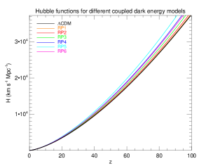
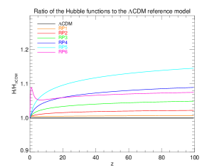
As pointed out in Sec. 2.1, the coupling modifies the background evolution through the existence of a phase – corresponding to the so called $\phi$MDE era in Amendola (2000) – in which the coupled matter fluid (CDM in our case) and the DE scalar field evolve with a constant energy density ratio (here we always assume the Universe to be flat such that $\Omega_{\rm tot}=1$). This leads to the presence of a non negligible Early DE component (EDE, Doran et al., 2001; Doran & Robbers, 2006) during the entire epoch of structure formation. The effect of such an EDE is to change the expansion history of the Universe, which has to be properly taken into account for the N-body time integration. In order to do so, we replaced the computation of the Hubble function $H(a)$ in GADGET-2 by a linear interpolation from a table of values of $H(a)$ precomputed for each model under investigation with the modified version of CMBEASY described above. The effect of the coupling on the expansion is shown in Fig. 1. We note that the same approach has also been adopted for the other relevant quantities described in Table 3, which were first computed numerically using CMBEASY, and then used as an input for our modified version of GADGET-2.

Figure 1: Left panel: Hubble functions as a function of redshift for the different coupled DE models with constant coupling investigated in this work and described in Table 2 as compared to $\Lambda$CDM (black curve). Right panel: Ratio of the Hubble functions of each coupled DE model to the Hubble function for the reference $\Lambda$CDM cosmology as a function of redshift.

Function	Meaning
$H(a)$	Hubble function
$\Delta G(a)$	Possible global variation of the gravitational constant
$\beta_{b}(\phi)$	Coupling function for the baryons
$\beta_{c}(\phi)$	Coupling function for CDM
$\Delta m_{b}$	Correction term for baryon particle masses
$\Delta m_{c}$	Correction term for CDM particle masses
$\Omega_{kin}(\phi)$	Dimensionless kinetic energy density of the scalar field

Table 3: List of input functions for the coupled DE implementation in GADGET-2.

3.1.2 Mass variation

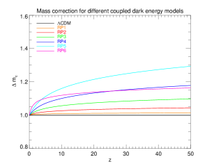
As described in Sec. 2.1, the coupled species feature an effective particle mass that changes in time. Consequently, the corresponding cosmological densities $\rho_{c}$ or $\rho_{b}$ will not be scaling anymore as $a^{-3}$, but will have a correction term arising from the variation of particle masses on top of the pure volume dilution. This correction depends on the scalar field dynamics, and takes the form of Eqn. (30). Then, if the particle masses in the simulation box are computed according to the cosmic densities $\Omega_{c,0}$ and $\Omega_{b,0}$ at the present time, they will need to be corrected at each timestep by a factor

$$\Delta m_{c}(a) = e^{-\int_{a}^{1}{\beta_{c}(\phi)\frac{{\rm d}\phi}{{\rm d}a}{\rm d}a}}\,,$$ (32)

$$\Delta m_{b}(a) = e^{-\int_{a}^{1}{\beta_{b}(\phi)\frac{{\rm d}\phi}{{\rm d}a}{\rm d}a}}\,.$$ (33)

Figure 2: Mass correction as a function of redshift for the coupled DE models with constant coupling.

In Fig. 2, we show the evolution with redshift of the correction term (32) for our set of models.

Although the coupled DE implementation for GADGET-2 that we present here in principle allows for a coupling also to baryons, such a coupling is tightly constrained by experimental tests of gravity on solar system scales (Damour et al., 1990). Therefore, in the coupled DE models we consider in this work, no coupling to baryons is considered, and baryon masses are always constant. However, even a very tiny coupling to baryons, in the range allowed by present bounds, could possibly play a significant role in cosmological models with multiple dark matter families (Huey & Wandelt, 2006), like for example the Growing Neutrino scenario introduced by Amendola et al. (2008). We plan to study detailed N-body simulations of this kind of models in forthcoming work.

3.1.3 Cosmological extra velocity-dependent acceleration

A further modification to the GADGET-2 code concerns the extra cosmological velocity-dependent term induced by the coupling in the Euler equation, as shown in Equations (28, 29). In standard cosmological simulations with GADGET-2 the usual cosmological velocity-dependent term (first term of Eqn. 29) is not directly computed because the choice of variables removes it from the acceleration equation. If we denote with ${\mn@boldsymbol{x}}$ comoving coordinates and with ${\mn@boldsymbol{r}}=a(t){\mn@boldsymbol{x}}$ physical coordinates, we have that:

$$\dot{{\mn@boldsymbol{r}}}=H{\mn@boldsymbol{r}}+{\mn@boldsymbol{v}}_{p}\,,\qquad{\mn@boldsymbol{v}}_{p}\equiv a(t)\dot{{\mn@boldsymbol{x}}}\,.$$ (34)

Instead of using the peculiar velocity ${\mn@boldsymbol{v}}_{p}$, GADGET-2 makes use of the variable ${\mn@boldsymbol{p}}\equiv a^{2}(t)\dot{{\mn@boldsymbol{x}}}$ (see Springel (2005) for more details), for which the following relation holds:

$$\dot{{\mn@boldsymbol{v}}}_{p}=\frac{1}{a}\dot{{\mn@boldsymbol{p}}}-\frac{H}{a}{\mn@boldsymbol{p}}\,.$$ (35)

It is then straightforward, by using Eqn. (35), to find a generalization of Eqn. (28) to a system of $N$ particles, in terms of the new velocity variable ${\mn@boldsymbol{p}}$:

$$\dot{{\mn@boldsymbol{p}}}_{i}=\frac{1}{a}\left[\beta_{\gamma}(\phi)\frac{\dot{\phi}}{M}a{\mn@boldsymbol{p}}_{i}+\sum_{j\neq i}\frac{\tilde{G}_{ij}m_{j}{\mn@boldsymbol{x}}_{ij}}{|{\mn@boldsymbol{x}}_{ij}|^{3}}\right]\,,$$ (36)

where $i$ and $j$ are indices that span over all the particles of the simulation, $\gamma=c,b$ for CDM or baryons respectively, and $\tilde{G}_{ij}$ is the effective gravitational constant between the $i$-th and the $j$-th particles, as determined in Eqn. (25) and whose implementation will be discussed below.

It is evident from Eqn. (36) that for zero coupling no cosmological velocity-dependent term is present in the acceleration equation, which is then just Newton’s law in comoving coordinates. In general, however, whenever a coupling is present, the additional term

$$a(\dot{{\mn@boldsymbol{p}}}+\Delta\dot{{\mn@boldsymbol{p}}})\equiv a\dot{{\mn@boldsymbol{p}}}+\beta_{\gamma}(\phi)\frac{\dot{\phi}}{M}a{\mn@boldsymbol{p}}_{i}$$ (37)

has to be explicitely added to the Newtonian acceleration of every particle. This term does not depend on the matter distribution in the rest of the Universe. It is therefore a purely cosmological drag that would be present also in absence of any gravitational attraction. It is interesting to notice that in the case of constant positive coupling and a monotonic scalar field potential as investigated here, the extra cosmological velocity-dependent term induces an acceleration in the same direction as the velocity of the particle. It therefore is effectively a “dragging” term, speeding up the motion of the particles.

Scalar field models where the dynamics of the field or the evolution of the coupling induce a change in the sign of $\beta_{i}(\phi)\dot{\phi}$, thereby changing the direction of this extra velocity-dependent force, will be studied in future work (Baldi & Macciò, in prep.).

3.1.4 Fifth force implementation

One of the most important modifications introduced by the coupling between DE and CDM is the presence of a modified gravitational constant, formally written as in Eqn. (25), for the gravitational interaction of CDM particles. In fact, if in general the substitution (Amendola, 2004)

$$G_{N}\rightarrow\tilde{G}_{lm}=G_{N}\cdot(1+2\beta_{l}\beta_{m})\,,$$ (38)

holds for each pair $(l,m)$ of particles, with $l$ and $m$ denoting the species of the particle, in our case only CDM-CDM interaction is affected, while baryon-CDM or baryon-baryon interactions remain unchanged since $\beta_{b}=0$. The dependence of this modified gravitational interaction on the particle type requires an N-body code to distinguish among different particle types in the gravitational force calculation. In GADGET-2, the gravitational interaction is computed by means of a TreePM hybrid method (see Springel, 2005, for details about the TreePM algorithm), so that both the tree and the particle-mesh algorithms have to be modified in order to account for this new phenomenology.

Tree algorithm modifications – In a standard tree algorithm, each node of the tree carries informations about the position of its centre of mass, its velocity, and its total mass. The decision whether to compute the force exerted on a target particle by the whole node or to further divide it into eight smaller nodes is made based on a specific opening criterion, which sets the accuracy threshold for approximating the gravitational potential of a distribution of particles with its low-order multipole expansion. Since in uncoupled cosmological models all particles interact with the same gravitational strength, as soon as the opening criterion is fulfilled the force is computed assigning all the mass contained in the node to its centre of mass. For coupled quintessence cosmologies, this is no longer accurate enough given that the different particle species will contribute differently to the gravitational force acting on a target particle. This means that besides the total mass and the total centre of mass position and velocity, each node has to carry information about the mass and centre-of-mass position and velocity of each particle species with different coupling.

Particle-Mesh algorithm modifications – In the Tree-PM algorithm, the long-range part of the gravitational force is computed by means of Fourier techniques. For coupled DE models, where different particle species interact with an effectively different gravitational force, the PM procedure has to be repeated as many times as there are differently interacting particle types, each time assigning to the cartesian grid only the mass in particles of a single type, and then computing the gravitational potential and the acceleration deriving from the spatial distribution of that particle species alone. In this way, the total force is built up as a sum of several partial force fields from each particle type.

3.1.5 Initial conditions

The initial conditions of a cosmological N-body simulation need to specify the positions and velocities of all the particles in the cosmological box at the starting redshift $z_{i}$ of the simulation. These quantities are usually computed by setting up a random-phase realization of the power spectrum of the studied cosmological model according to the Zel’dovich approximation (Zel’dovich, 1970). The normalization amplitude of the power spectrum is adjusted such that the linearly evolved rms-fluctuations $\sigma_{8}$ on a top-hat scale of $8\,h^{-1}{\rm Mpc}$ at a given redshift $z_{\rm norm}$ (usually chosen to be $z_{\rm norm}=0$) have a prescribed amplitude.

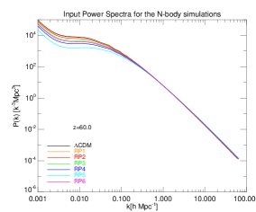
The coupling between DE and CDM can have a strong impact on the transfer function of matter density fluctuations, as first pointed out by Mainini & Bonometto (2007b). For this reason we compute the required initial power spectrum directly with the modified Boltzmann code CMBEASY, because the phenomenological parameterizations of the matter power spectrum available for the $\Lambda$CDM cosmology (e.g. Bardeen et al., 1986; Eisenstein & Hu, 1998) would not be accurate enough. The resulting effect on the power spectrum is shown in Fig. 3 for the different models considered in our set of simulations.

Figure 3: Matter power spectra at $z=60$ for interacting DE models with constant coupling as computed by CMBEASY.

Once the desired density field has been realized with this procedure, the displacements of the particles from the grid points need to be rescaled with the linear growth factor $D_{+}$ for the cosmological model under investigation between the redshifts $z_{\rm norm}$ and $z_{i}$ in order to set the correct amplitude of the power spectrum at the starting redshift of the simulation. Also, the velocities of the particles are related to the local overdensities according to linear perturbation theory, via the following relation, here written in Fourier space:

$${\mn@boldsymbol{v}}({\mn@boldsymbol{k}},a)=if(a)aH\delta({\mn@boldsymbol{k}},a)\frac{{\mn@boldsymbol{k}}}{k^{2}}\,,$$ (39)

where the growth rate $f(a)$ is defined as

$$f(a)\equiv\frac{d\ln D_{+}}{d\ln a}\,.$$ (40)

This requires an accurate calculation of the linear growth function $D_{+}(z)$ for the coupled model, which we again compute numerically with CMBEASY.

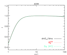
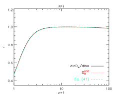
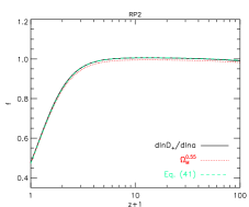
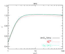
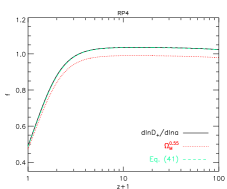
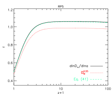
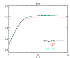
We note that a phenomenological parameterization of the growth function for coupled DE models with constant coupling to dark matter has recently been made available by Di Porto & Amendola (2008). However, it is only valid for models with no admixture of uncoupled matter, whereas in our case we also have a baryonic component. Also, in the $\Lambda$CDM cosmology, the total growth rate is well approximated by a power of the total matter density $\Omega_{M}^{\gamma}$, with $\gamma=0.55$, roughly independently of the cosmological constant density (Peebles, 1980). This is however no longer true in coupled cosmologies, as we show in Fig. 4. We find that, for our set of coupled DE models, a different phenomenological fit given by

$$f(a)\sim\Omega_{M}^{\gamma}(1+\gamma\frac{\Omega_{\rm CDM}}{\Omega_{M}}\epsilon_{c}\beta_{c}^{2})\,,$$ (41)

with $\gamma=0.56$ (as previously found in Amendola & Quercellini, 2004) and $\epsilon_{c}=2.4$ works well. The fit (41) reproduces the growth rate with a maximum error of $\sim 2\%$ over a range of coupling values between $0$ and $0.2$ and for a cosmic baryon fraction $\Omega_{b}/\Omega_{m}$ at $z=0$ in the interval $0.0-0.1$ for the case of the potential slope $\alpha=0.143$ (corresponding to the slope of the RP1-RP5 models). For a value of $\alpha=2.0$ (corresponding to the slope assumed for RP6) the maximum error increases to $\sim 4\%$ in the same range of coupling and baryon fraction. In Fig. 4, we plot both the fitting formulas together with the exact $f(a)$. For our initial conditions setup we in any case prefer to use the exact function $f(a)$ directly computed for each model with CMBEASY, rather than any of the phenomenological approximations.

Figure 4: Comparison of the function $f(a)$ with its usual approximation $f=\Omega_{m}^{0.55}$ and with the new fit of Eqn. (41) for a $\Lambda$CDM model and for a series of coupled DE models.

3.2 Tests of the numerical implementation: the linear growth factor

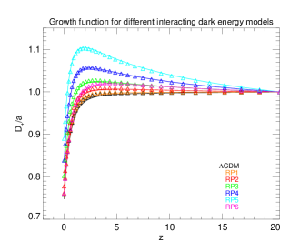
As a first test of our implementation we check whether the linear growth of density fluctuations in the simulations is in agreement with the linear theory prediction for each coupled DE model under investigation. To do so, we compute the growth factor from the simulation outputs of the low-resolution simulations described in Table 2 by evaluating the change in the amplitude of the matter power spectrum on very large scales, and we compare it with the solution of the system of coupled equations for linear perturbations (19), numerically integrated with CMBEASY. The comparison is shown in Fig. 5 for all the constant coupling models. The accuracy of the linear growth computed from the simulations in fitting the theoretical prediction is of the same order for all the values of the coupling, and the discrepancy with respect to the numerical solution obtained with our modified version of GADGET-2 never exceeds a few percent.

Figure 5: Evolution of the growth function with redshift for the seven models of coupled DE investigated with the low-resolution simulations ran with our modified version of GADGET-2. The solid lines are the total growth functions as evaluated numerically with CMBEASY, while the triangles are the growth function evaluated from the simulations. The relative accuracy in reproducing the theoretical prediction is of the order of a few percent irrespective of the coupling value $\beta_{c}$.

3.3 Our set of N-body simulations

In our simulations, we are especially interested in the effects that the presence of a coupling between DE and CDM induces in the properties of collapsed structures, and we would like to understand which of these effects are due to linear features of the coupled theory, and which due to the modified gravitational interaction in the dark sector. This goal turns out to be challenging due to the presence of several different sources of changes in the simulation outcomes within our set of runs. To summarize this, let us briefly discuss in which respect, besides the different gravitational interactions, the high-resolution simulations listed in Table 2 are different from each other:

• the initial conditions of the simulations are generated using a different matter power spectrum for each model, i.e. the influence of the coupled DE on the initial power spectrum is taken into account and this means that every simulation will have a slightly different initial power spectrum shape;

• the amplitude of density fluctuations is normalized at $z=0$ for all the simulations to $\sigma_{8}=0.796$, but due to the different shapes of the individual power spectra the amplitude of density fluctuations at the present time will not be the same in all simulations at all scales;

• the initial displacement of particles is computed for each simulation by scaling down the individual power spectrum amplitudes as normalized at $z=0$ to the initial redshift of the simulations ($z_{i}=60$) by using for each simulation the appropriate growth function. This results in a lower initial amplitude for more strongly coupled models;

• hydrodynamical forces are acting on baryon particles in all the four fully self-consistent simulations ($\Lambda$CDM, RP1, RP2, RP5), and therefore differences in the evolution of the dark matter and baryon distributions might be due to a superposition of hydrodynamics and modified gravitational interaction;

• non-adiabatic processes like e.g. radiative cooling, star formation, and feedback are not included in any of the simulations presented in this work.

In order to try to disentangle which of these differences cause significant changes in our results, we decided to run three further test simulations in which, in turn, some of the new physics has been disabled.

• In the two simulations labelled as “NO-SPH” ($\Lambda$CDM-NO-SPH, RP5-NO-SPH), we disabled hydrodynamical SPH (Smoothed Particle Hydrodynamics) forces in the code integration. We can then compare a $\Lambda$CDM model with a strongly coupled model treating both baryons and cold dark matter particles as collisionless particles. The differences in the dynamics will then be due only to the different gravitational interaction implemented in the RP5 model. However, the shape and amplitude of the initial power spectrum for the two simulations are still different;

• In the simulation labelled RP5-NO-GF, we ran a RP5 cosmological model using as initial conditions the same file we used for the $\Lambda$CDM run. This means that no effect arising in this simulation compared to $\Lambda$CDM can be due to different initial conditions, i.e. due to the differences in the shape and amplitude of the initial power spectra that are present in the other simulations.

4 Results

We now describe our results for the effect of the coupling between DE and CDM on nonlinear structures. As first basic analysis steps we apply the Friends-of-Friends (FoF) and SUBFIND algorithms (Springel et al., 2001) to identify groups and gravitationally bound subgroups in each of our simulations. Given that the seed used for the random realization of the power spectrum in the initial conditions is the same for all the seven simulations, structures will form roughly at the same positions in all simulations, and it is hence possible to identify the same objects in all the simulations and to compare their properties. Nevertheless, due to the different timestepping induced by the different physics implemented in each run, and the slightly different transfer functions, objects in the different simulations can be slightly offset from each other. We therefore apply a selection criterion and identify objects found in the different simulations as the same structure only if the most bound particle of each of them lies within the virial radius of the corresponding structure in the $\Lambda$CDM simulation. If this criterion is not fulfilled for all the different simulations we want to compare, we do not consider the corresponding halo in any of the comparison analysis described below. We restrict this matching procedure to the 200 most massive halos identified by the FoF algorithm, which have virial masses ranging from $4.64\times 10^{12}h^{-1}M_{\odot}$ to $2.83\times 10^{14}h^{-1}M_{\odot}$. Note that depending on the specific set of simulations we consider in our comparative analysis, this can result in small differences in the number of halos included in each of the comparison samples.

4.1 Halo mass function

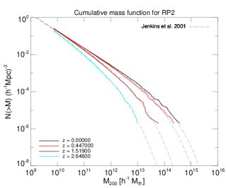
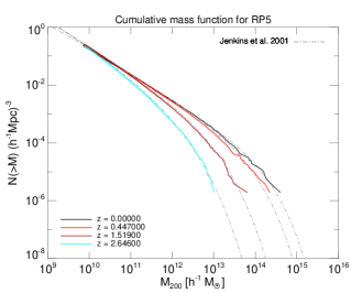
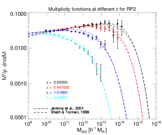
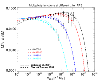
For the four fully self-consistent high-resolution simulations listed in Table 2 ($\Lambda$CDM, RP1, RP2, RP5), we have computed the halo mass function based on the groups identified with the Friends-of-Friends (FoF) algorithm with a linking length of $\lambda=0.2\times\bar{d}$, where $\bar{d}$ is the mean particle spacing. It is important to recall that our simulations have the same initial random phases and are normalized to the same $\sigma_{8}$ today, but the shapes of the input power spectra are slightly different for each simulation. In Fig. 6 we plot the cumulative mass functions for the four simulations at different redshifts. Remarkably, the mass functions of all the cosmological models and at all the different redshifts considered are well fit by the formula given in Jenkins et al. (2001), provided it is evaluated with the actual power spectrum and the correct linear growth factor for the corresponding cosmological model. The usual mass function formalism hence continues to work even for coupled DE cosmologies, a result in line with recent findings for early dark energy cosmologies (Grossi & Springel, 2008; Francis et al., 2008a, b).

Figure 6: Cumulative mass functions for the four fully self-consistent high-resolution simulations of the coupled DE models. The four differently-coloured solid lines in each figure represent the cumulative mass function at four different redshifts in each of the investigated models. The dot-dashed lines are the corresponding predictions according to the Jenkins et al. (2001) formula, computed for each simulation with the appropriate growth function and power spectrum.

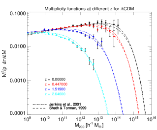
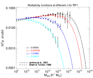
We also plot in Fig. 7 the multiplicity function, defined as the derivative of the mass function with respect to the mass ($M^{2}/\rho\cdot{\rm d}n(<M)/{\rm d}M$), for each simulation at different redshifts. This more sensitive representation of the mass function reveals a slightly better agreement with the formula by Sheth & Tormen (1999) compared with that of Jenkins et al. (2001), which are both overplotted for a direct comparison.

Figure 7: Multiplicity functions for the four high-resolution simulations of the interacting DE models. The four differently-coloured sets of data points are the multiplicity functions evaluated in equally spaced logarithmic mass bins at four different redshifts. The dot-dashed and dashed lines represent the predictions for the multiplicity function from Jenkins et al. (2001) and Sheth & Tormen (1999), respectively, computed for each simulation with the appropriate growth function and power spectrum. The comparison clearly shows a slightly better agreement with the fitting function by Sheth & Tormen (1999), in particular at high redshift.

4.2 Matter power spectrum

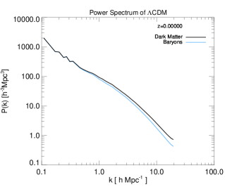
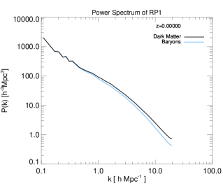
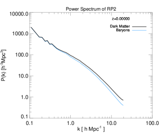
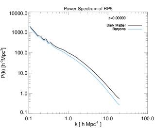
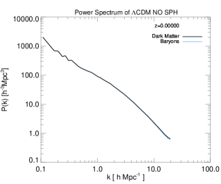
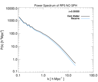
The presence of a long-range fifth-force acting only between CDM particles induces a linear bias on all scales between the amplitude of density fluctuations in baryons and CDM. These density fluctuations, in fact, start with the same relative amplitude in the initial conditions of all the simulations, and then grow at a different rate due to the presence of the extra force. Such a bias is then easily distinguishable from the hydrodynamical bias that develops only at small scales as structure evolves. This effect is clearly visible in our simulations, as it can be seen from the baryon and CDM power spectra at $z=0$ in the four different cosmologies we analyze (Fig. 8): the density power spectra of baryons and CDM end up with a different amplitude on all scales at $z=0$ in the coupled DE models. CDM always has a larger amplitude, and the difference grows with increasing coupling $\beta_{c}$.

In order to disentangle this effect from the small scale bias due to pressure forces acting on baryons, we can make use of our “NO-SPH” simulations to show the result if only the fifth-force effect is included. This is shown in the last two panels of Fig. 8.

Figure 8: Power spectra of CDM (black line) and baryons (blue line) at $z=0$ for the set of coupled DE models under investigation. The appearance of a bias between the two distributions, which grows with increasing coupling $\beta_{c}$, is clearly visible at the large scale end of the plots. The last two panels show the comparison of a $\Lambda$CDM and a coupled DE cosmology with $\beta_{c}=0.2$ in absence of hydrodynamic forces acting on baryons. In these two panels, the bias on all scales is purely due to the interaction of CDM with the DE scalar field $\phi$.

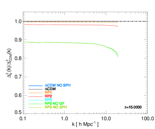
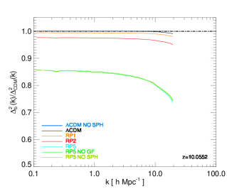
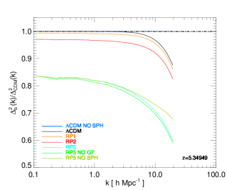
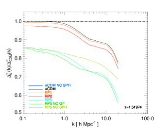
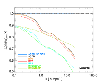
In order to make the effect described above even more visible, and to better show the difference of the hydrodynamical bias from the gravitational one induced by the coupled DE component, we also plot in Fig. 9 the ratio of the power $\Delta^{2}(k)=P(k)k^{3}/2\pi$ in baryons to that in CDM at different redshifts. In these plots, we have corrected all the curves for a spurious effect on small scales due to the mass difference between baryon and CDM particles in the simulations that induces a small drop in the baryon power. This effect is of purely numerical origin and could be easily removed by using particles of equal mass for the two cosmological matter species in the N-body runs.

Let us now briefly comment on the plots of Fig. 9. The curves represent the bias between the baryon and the CDM density fluctuation amplitudes as a function of the wave number. A constant bias of 1.0 at all redshifts is the expected result for two collisionless matter species interacting with the same gravitational strength, and this is what we find for our $\Lambda$CDM-NO-SPH simulation (dark blue curve). In the $\Lambda$CDM simulation, we notice that this value of 1.0 is maintained at all redshifts only for large scales, while on smaller scales, as structures evolve, the collisional nature of baryon particles progressively induces a drop of this ratio (black curve). The same behaviour is seen for all the other hydrodynamic simulations (RP1, RP2, RP5). However, in the latter cases, the large-scale bias is always smaller than 1.0, already at high redshifts, and it decreases with increasing values of the CDM coupling $\beta_{c}$, as expected. This is the gravitational bias that appears also at large scales in Fig. 8.

Particularly interesting is then again the case of the RP5-NO-SPH simulation (dark-green curve), as compared to the $\Lambda$CDM-NO-SPH one, because it allows us to disentangle the hydrodynamic effects from the effects due to the coupled DE extra physics. In this case we find that the bias of RP5-NO-SPH perfectly overlaps with the one of the other two RP5 simulations at high redshifts, while at lower and lower redshifts, the small scale behaviour is progressively more and more different: as expected the absence of hydrodynamic forces acting on baryon particles induces a larger value of the bias, which is now solely due to the different gravitational strength felt by the two particle species. It is however very interesting to notice that the bias does not keep the large-scale linear value at all scales, as it is the case for the $\Lambda$CDM-NO-SPH run, but evolves towards lower and lower values for smaller and smaller scales. This clearly shows that nonlinearities enhance the effect of the coupling on the growth of overdensities in the two differently interacting matter species.

Figure 9: Ratio of the power spectra of baryons and CDM as a function of wavenumber for the set of high-resolution simulations ran with our modified version of GADGET-2, for five different redshifts. The linear large-scale bias appears already at high redshifts, while at lower redshifts the hydrodynamic forces start to suppress power in the baryon component at small scales. In absence of such hydrodynamic forces the progressive enhancement of the large scale bias at small scales for the RP5-NO-SPH run (light green curve) as compared to the completely flat behaviour of the $\Lambda$CDM-NO-SPH simulation (blue curve) – where no bias is expected – shows clearly that nonlinearities must increase the effect of the coupling on the different clustering rates of the two species. All the curves have been corrected for a spurious numerical drop of the baryonic power at small scales as described in the text.

4.3 Halo density profiles

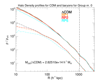
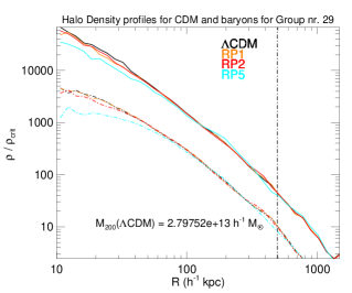
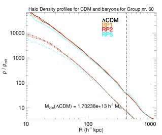
Applying the selection criterion described above to our four self-consistent simulations ($\Lambda$CDM, RP1, RP2, RP5) we select among the 200 most massive groups identified at $z=0$ for each run 74 objects that can be considered with certainty to be the same structure in the different simulations. For these 74 halos we compute the spherically averaged density profiles of CDM and baryons as a function of radius around the position of the particle with the minimum gravitational potential.

Interestingly, the halos formed in the coupled DE cosmologies show systematically a lower inner overdensity with respect to $\Lambda$CDM, and this effect grows with increasing coupling. This is clearly visible in Fig. 10 where we show the density profiles of CDM and baryons in the four different cosmologies for a few selected halos of different virial mass in our sample. We remark that this result is clearly incompatible with the essentially opposite behaviour previously reported by Macciò et al. (2004), and deserves a more detailed discussion.

Figure 10: Density profiles of CDM (solid lines) and baryons (dot-dashed lines) for four halos of different mass in the simulation box at $z=0$. The vertical dot-dashed line indicates the location of the virial radius for the $\Lambda$CDM halo. The decrease of the inner overdensity of the profiles with increasing coupling is clearly visible in all the four plots.

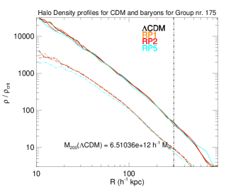
Unlike found in Macciò et al. (2004), all the 74 halos in our comparison sample have density profiles that are well fitted by the NFW fitting function (Navarro et al., 1997)

$$\frac{\rho(r)}{\rho_{\rm crit}}=\frac{\delta^{*}}{({r}/{r_{s})}(1+{r}/{r_{s}})^{2}}\,,$$ (42)

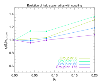
independent of the value of the coupling. Here $\delta^{*}$ is a parameter that sets the characteristic halo density contrast relative to the critical density $\rho_{\rm crit}$. The scale radius $r_{s}$ increases for each halo with increasing coupling $\beta_{c}$, and becomes larger than that found in $\Lambda$CDM. In other words, the halos become less concentrated with increasing coupling.

For example, for the four halos shown in Fig. 10, the scale radius grows with increasing coupling by roughly 10% to 35% going from $\Lambda$CDM to RP5, as listed in Table 4, and shown in Fig. 11. The effect is not strong enough to fully address the “cusp-core” problem, but clearly shows how the interaction between DE and CDM can produce shallower halo density profiles with respect to a $\Lambda$CDM cosmology with the same cosmological parameters. This result goes then in the direction of alleviating the problem, and therefore opens up new room for the study of dark interactions as opposite to previous claims. In fact, although the models presented here span over the full observationally allowed parameter space for constant-coupling models (Bean et al. (2008), but see also e.g. La Vacca et al. (2009)), it is well conceivable that more realistic scenarios with a variable coupling strength could produce larger effects in the nonlinear regime without running into conflict with present observational bounds from linear probes. We defer to future work the investigation of such models, but we stress here that our present results constitute the first evidence that the nonlinear dynamics of generalized coupled cosmologies might provide a solution to the “cusp-core” problem.

	Group 0 $r_{s}$ (h-1 kpc)	Group 0 $\frac{r_{s}}{r_{s}(\Lambda\mathrm{CDM})}$	Group 29 $r_{s}$ (h-1 kpc)	Group 29 $\frac{r_{s}}{r_{s}(\Lambda\mathrm{CDM})}$	Group 60 $r_{s}$ (h-1 kpc)	Group 60 $\frac{r_{s}}{r_{s}(\Lambda\mathrm{CDM})}$	Group 175 $r_{s}$ (h-1 kpc)	Group 175 $\frac{r_{s}}{r_{s}(\Lambda\mathrm{CDM})}$
$\Lambda$CDM	225.14	1.0	105.51	1.0	61.92	1.0	70.61	1.0
RP1	229.00	1.02	120.21	1.14	61.16	0.99	67.45	0.96
RP2	233.96	1.04	119.68	1.13	63.52	1.03	70.48	1.0
RP5	295.47	1.31	143.92	1.36	73.46	1.19	76.26	1.08

Table 4: Evolution of the scale radius $r_{s}$ for the four halos shown in Fig. 10 with respect to the corresponding $\Lambda$CDM value. The trend is towards larger values of $r_{s}$ with increasing coupling $\beta_{c}$, with a relative growth of up to 36% for the largest coupling value $\beta_{c}=0.2$.

Figure 11: Relative evolution with respect to $\Lambda$CDM of the scale radius $r_{s}$ for the four halos plotted in Fig. 10 as a function of coupling $\beta_{c}$.

4.4 Halo concentrations

For all the 200 most massive halos found in each of our four fully self consistent simulations we compute halo concentrations as

$$c=\frac{r_{\rm 200}}{r_{s}}\,,$$ (43)

based on our NFW fits to the halo density profiles. Here $r_{\rm 200}$ is the radius enclosing a mean overdensity 200 times the critical density. Note that here no further selection criterion is applied, and the concentration is computed for all the 200 most massive halos in each simulation.

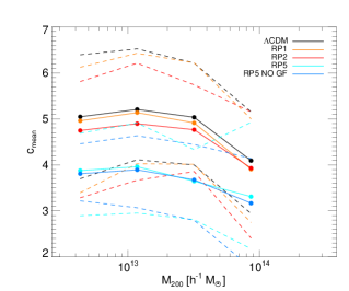
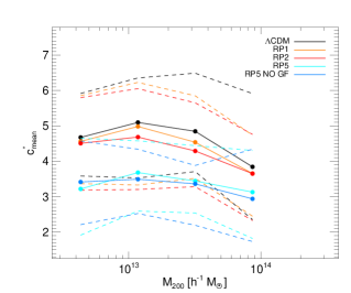
Consistently with the trend found for the inner overdensity in the halo density profiles and for the evolution of the scale radius with coupling, we find that halo concentrations are on average significantly lower for coupled DE models with respect to $\Lambda$CDM, and the effect again increases with increasing coupling $\beta_{c}$. This behaviour is shown explicitly in the left panel of Fig. 12, where we plot halo concentrations as a function of the halo virial mass $M_{200}$ for a series of our high-resolution simulations. In the standard interpretation, the halo concentrations are thought to reflect the cosmic matter density at the time of formation of the halo, leading to the association of a larger value of the concentration with an earlier formation epoch, and vice versa. In the context of this standard picture, the effect we found for the concentrations could be interpreted as a sign of a later formation time of massive halos in the coupled DE models as compared to the $\Lambda$CDM model. Such a later formation time could be possibly due to the fact that matter density fluctuations start with a lower amplitude in the initial conditions of the coupled cosmologies with respect to $\Lambda$CDM, and this would make them forming massive structures later, despite their faster linear growth (as shown in Fig. 5).

However, we can demonstrate that this is not the case, just making use of our RP5-NO-GF simulation, in which the Universe evolves according to the same physics as RP5, but starting with the identical initial conditions as used for the $\Lambda$CDM run. Therefore, any difference between these two simulations can not be due to the initial amplitude of fluctuations. The evolution of halo concentrations with mass for this run is also plotted in Fig. 12 (dark blue curve), and shows a very similar behaviour to the RP5 curve.

As a cross check of this result, we have repeated the same analysis by computing halo concentrations with an independent method that circumvents the profile fitting. The concentration can be related to two other basic structural properties of a halo, namely its maximum rotational velocity $V_{\rm max}$, and the radius at which this velocity peak is located, $r_{\rm max}$. According to Springel et al. (2008), the concentration can then be related to these two quantities by the relation:

$$\frac{200}{3}\frac{c^{3}}{\ln(1+c)-c/(1+c)}=7.213\,\delta_{V}\,,$$ (44)

where $\delta_{V}$ is a simple function of $V_{\rm max}$ and $r_{\rm max}$:

$$\delta_{V}=2\left(\frac{V_{\rm max}}{H_{0}r_{\rm max}}\right)^{2}\,.$$ (45)

We denote the concentrations evaluated in this way as $c^{*}$, and include our results as a function of halo mass in the right panel of Fig. 12. Although not identical in detail, as expected due to the different methods used to measure concentrations, the two plots of Fig. 12 show the same trend for the evolution of halo concentrations with coupling, and the same independence of this effect from the initial conditions of the simulations. The slight down-turn of the concentrations curve at the low-mass end that is visible in both the two panels of Fig. 12 is an expected effect due to numerical resolution, as was discussed in detail in Neto et al. (2007) and in Springel et al. (2008). Although the concentration decrease is found to have the same trend and amplitude for the poorly resolved low-mass halos as for the larger structures for which no resolution problem is expected, one should keep in mind as an element of caution that higher resolution simulations would be required for a definitive confirmation of this effect in the low-mass range of our comparison sample, i.e. for masses below $10^{13}$ M_⊙/h.

Figure 12: Evolution of the mean halo concentration as a function of mass for the 200 most massive halos in our simulations and for the different cosmological models under investigation. The concentrations have been computed by directly fitting the halo density profile of each halo with an NFW model (left panel) or by using the method introduced by Springel et al. (2008) and described in Eqs. (44,45) (right panel). The halos have been binned by mass, and the mean concentration in each bin is plotted as a filled circle. The coloured dashed lines indicate for each simulation the spread of 68% of the halos in each mass bin. The highest mass bin is not plotted because of its very low number of halos. The decrease of the mean concentration with increasing coupling appears in the same way in both plots.

In order to directly verify that the lower concentrations cannot be a consequence of a later formation time we have also computed the average formation redshift of the halos in our sample for all the four self-consistent simulations, by building merger trees for all the halos in our sample, and by following backwards in time the main progenitor of each halo until the redshift at which its virial mass is only half of the final virial mass of the halo at $z=0$. We define the corresponding time as the formation redshift $z_{f}$ of the halo.

Figure 13: Evolution of the mean halo formation redshift $z_{f}$ as a function of halo mass for the 200 most massive halos in our simulations and for the different cosmological models under investigation. The formation redshift $z_{f}$ is defined as the redshift at which the main progenitor of the halo has a virial mass equal to half the virial mass of the halo at $z=0$. The halos have been binned by mass, and the mean formation redshift in each bin is plotted as a filled circle. The coloured dashed lines indicate for each simulation the spread of 68% of the halos in each mass bin. The highest mass bin is not plotted because of its too low number of halos.

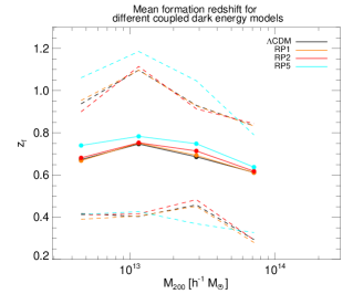
In Figure 13, we show the evolution of $z_{f}$ as a function of halo mass for all our cosmological models. It is evident that massive halos in the different cosmologies form approximately at the same time, with a slightly earlier formation for the RP5 cosmology, which one might have expected to translate into slightly larger values of the concentrations. Therefore we conclude that the unambiguous trend of lower halo concentrations for larger coupling values must be a peculiar feature that arises from the extra physics that characterizes the coupled DE cosmologies. A more detailed investigation of how this peculiar behaviour arises is hence required in order to understand this phenomenology of the dynamics in coupled DE cosmologies.

We perform such an investigation by switching off individually the two main effects which could be responsible of the concentrations drop, which are the variation of particle mass and the extra velocity-dependent term. To save computational time, we do this only for the most strongly coupled model RP5 and only for the late stages of cosmic evolution. More specifically, we take one of our RP5 simulation snapshots at a given redshift $z^{*}$, and use it as initial conditions file for a new run starting at $z=z^{*}$ down to $z=0$ in which one of these two effects is switched off. We label these simulations as “RP5-NO-MASS” and “RP5-NO-FRIC” for the cases where the mass decrease or the velocity-dependent term are dropped, respectively. We set $z^{*}=1.5$ as a conservative choice based on the consideration that, according to our definition of formation redshift of a halo, all the halos in our sample have a formation redshift $z<z^{*}$, as shown in Fig. 13.

By switching off the mass variation for $z<z^{*}$, we find that the halo concentrations at $z=0$ show a slight increase over the whole mass range of the sample with respect to the fully self-consistent RP5 simulation. This effect is shown in the left panel of Fig. 14. We interpret this as a sign of the fact that the mass decrease reduces the total gravitational potential energy of halos, resulting in a modification of their virial equilibrium configuration.

Figure 14: Evolution of halo concentrations for the same models and the same halo sample as in Fig. 12, and for an additional test simulation in each of the two panels. In the left panel, the simulation RP5-NO-MASS shows the effect of switching off the mass correction for $z<z^{*}\sim 1.5$: there is a small but systematic increase of average halo concentrations over the whole mass range. In the right panel, the simulation RP5-NO-FRIC shows the effect of switching off in the same redshift interval the velocity-dependent term. The increase of concentrations is in this case much more consistent and accounts for a large fraction of the total concentration reduction of RP5.

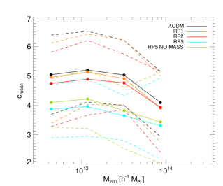
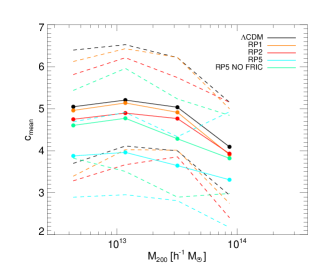
In fact, if the potential well of a halo gets shallower as time goes by as a consequence of the decrease of the mass of its CDM content, the system will find itself with an excess of kinetic energy, and will therefore expand in order to restore virial equilibrium. Such an expansion is expected to cause a drop of the halo concentrations, which we confirm here because switching off this mechanisms yields consistently higher concentrations at $z=0$. However, it is clear from Fig. 14 that this mechanism cannot account for the total effect of concentration decrease, but only for a small fraction of it.

We therefore now investigate the other possible origin of this effect, i.e. the impact of the velocity-dependent term (29) on the dynamics of CDM particles. To this end we switch off for $z<z^{*}$ the additional acceleration arising from the velocity-dependent term for coupled particles described by Eqn. (3.1.3). The outcome of this test simulation is shown in the right panel of Fig. 14: the increase of the concentrations with respect to the fully self-consistent RP5 simulation is now much more substantial than in the case of RP5-NO-MASS, and shows that the velocity-dependent term is actually the dominant mechanism in determining the decrease of halo concentrations and the decrease of the inner overdensity of CDM halos discussed above. The interpretation of this effect seems quite unambiguous: the velocity-dependent term induces an extra acceleration on coupled particles in the direction of their velocity, and this produces an increase of the kinetic energy of the particles, moving the system out of its virial equilibrium configuration. The system responds by a small expansion and a lowering of the concentration.

As a further check of this interpretation of our results, we also test directly the dynamic evolution of halos to check whether they really slightly expand in the presence of DE-CDM coupling. To this end, we compute for all the halos in our sample the time evolution of the mass and the number of particles contained in a sphere of physical radius $r=20\,h^{-1}\mathrm{kpc}$ centred on the potential minimum of each halo. This sphere represents the very innermost part of all the halos in our sample at any redshift between $z^{*}$ and 0, and we refer to it as the halo “core”; its mass content is expected to be roughly constant for $\Lambda$CDM cosmologies at low redshifts. Indeed, we can recover this behaviour for our $\Lambda$CDM simulation by averaging the evolution of core masses and particle numbers over the whole halo sample. On the other hand, for RP5, as expected according to our interpretation, both the mass and the number of particles in the halo cores strongly decrease with time. This is shown in Fig. 15, where the solid lines represent the average evolution of mass, and the dashed lines represent the average evolution of the particle number. Evidently, for $\Lambda$CDM the two curves coincide because the mass of the particles is constant and any change of the enclosed mass in the core must be due to a change of the number of enclosed particles. On the other hand, for RP5, the mass and the particle number behave differently due to the mass variation of CDM particles. The decrease of the number of particles contained in the core can be interpreted as a manifestation of an expansion of the halos. Moreover, if we compute the same evolution for our RP5-NO-FRIC simulation, we find an almost constant evolution of the core particle number and a very weak decrease of the core mass due to the variation of CDM particle mass. This result also confirms our interpretation concerning the origin of the decrease of concentrations: the velocity-dependent term is the most relevant mechanism for inducing halos expansion at low redshifts, and as a consequence the decrease of the inner overdensity of CDM halos and of their concentration.

Figure 15: Evolution with respect to the scale factor $a$ of the average mass (solid) and of the average number of particles (dashed) enclosed in a sphere of physical radius $r=20\mathrm{h}^{-1}\mathrm{kpc}$ centred on the potential minimum of each halo in our sample. The curves are normalized at $a=0.48$ ($z\sim 1$) and show the expected flat behaviour for the $\Lambda$CDM case (black line) for which the solid and the dashed curves coincide due to the constancy of the mass of particles. For the RP5 case (light blue curves), there is a strong decrease in time of both mass and particle number, which clearly illustrates the expansion of RP5 halos with respect to the $\Lambda$CDM case. By switching off the extra velocity-dependent force acting on CDM particles (RP5-NO-FRIC, light green curves), an almost flat behaviour is recovered again for the particle number, while the decrease of mass is now due to the particle mass variation – which is still in place for this simulation – on top of the particle number evolution. This plot therefore clearly shows that the extra physics of coupled DE cosmologies induces an overall expansion of CDM halos at low redshifts, and clearly identifies in the velocity-dependent

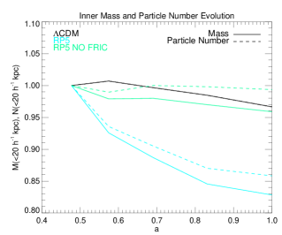
term the leading mechanism that produces this expansion.

While further investigations of these effects are certainly required in order to understand all the potential phenomenological features of interacting DE models, our conclusion that a coupling between DE and CDM produces less peaked halo density profiles and lower halo concentrations seems to be quite robust based on the analysis of our simulations that we have discussed here. We note again that our findings are in stark contrast with the results of previous work by Macciò et al. (2004) who found for coupled DE models a strong increase in concentration and density profiles in the centre that more steeply rise than $\Lambda$CDM. The effects we find go in the direction of less “cuspyness” of halo density profiles, which is preferred by observations and thus in fact opens up new room for the phenomenology of interacting DE models.

4.5 Integrated bias and halo baryon fraction

The extra force felt by CDM particles induces, as we have already seen for the evolution of the matter power spectrum, a bias in the evolution of density fluctuations of baryons and CDM (Mainini, 2005; Mainini & Bonometto, 2006; Manera & Mota, 2006). We can then use our selected halo sample to test the evolution of this bias from the linear regime already probed by the power spectrum on large scales to the highly nonlinear regime in the centre of massive collapsed structures. We then test the evolution of the integrated bias

$$B(<r)\equiv\frac{\rho_{b}(<r)-\bar{\rho}_{b}}{\bar{\rho}_{b}}\cdot\frac{\bar{\rho}_{c}}{\rho_{c}(<r)-\bar{\rho}_{c}}\,,$$ (46)

as defined in Macciò et al. (2004), where $\rho_{b}(<r)$ and $\rho_{c}(<r)$ are the densities within a sphere of radius $r$ around the potential minimum of a halo, for baryons and CDM, respectively. Following Macciò et al. (2004), we have not used the innermost part of the halos ($r<10h^{-1}{\rm kpc}\sim 3\times\epsilon_{s}$) in order to avoid potential resolution problems.

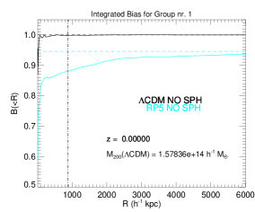
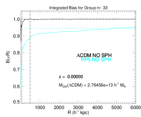
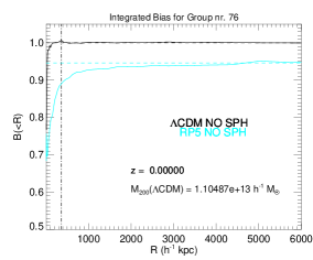
In Figure 16, we show the evolution of the bias for four selected halos of our sample with similar masses as the ones shown in Fig. 10. It clearly appears that the bias is considerably enhanced in the nonlinear regime, while at large scales it converges to the linear value evaluated from the power spectrum amplitude on large scales, represented in Fig. 16 by the horizontal dashed lines.

Figure 16: Evolution of the integrated bias $B(<r)$ for the four fully self-consistent high-resolution simulations and for four selected halos of different mass in our sample. The horizontal dashed lines indicate the value of the large scale linear bias as evaluated from the power spectrum amplitudes of baryons and CDM. The vertical black dot-dashed line shows the position of the virial radius for the $\Lambda$CDM halo in the sample. The drop of the value of $B(<r)$ in the innermost regions of the halos is evident but in these runs is given by a superposition of effects due to hydrodynamical forces and to the modified gravitational interaction. On large scales, the bias tends to converge to the linear value, as expected.

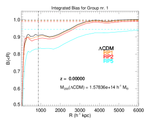
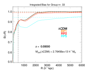
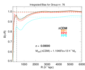
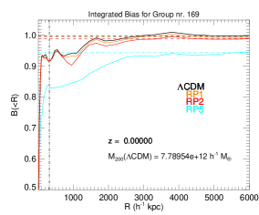
However, also in this case this effect could be due only to the presence of hydrodynamical forces acting on the baryons, and may not really be caused by the fifth-forces from the coupled DE scalar field, as we can infer from the fact that also the $\Lambda$CDM curve, where no coupled DE is present, shows a departure from the large scale value of 1.0 when approaching the centre of the halos. Once again we make use of our additional test simulations $\Lambda$CDM-NO-SPH and RP5-NO-SPH in order to disentangle the two effects. In Fig. 17, we show the same four plots as in Fig. 16 for the two simulations without hydrodynamic forces, and the appearance of a nonlinear bias imprinted only by the coupled DE scalar field acting on CDM particles is then absolutely evident. On the other hand, the absence of any bias, as expected, in the $\Lambda$CDM-NO-SPH run shows clearly that no major numerical problems can be responsible for the effect in the RP5-NO-SPH simulations. This evolution of the bias $B(<r)$ with radius for massive halos is in good agreement with that found by Macciò et al. (2004) despite the starkly different behavior of the individual overdensities in baryons and CDM found in the two works.

Figure 17: Evolution of the integrated bias $B(<r)$ for the two high-resolution simulations without hydrodynamical forces on baryon particles for the same four halos shown in Fig. 16. The enhancement of the bias due to the extra scalar force in the core of highly nonlinear structures appears here clearly.

It is interesting that the above effect produces a baryon deficit in virialized halos, i.e. they contain fewer baryons than expected based on their mass and the universal cosmological baryon fraction. In particular, this means that one can not expect that baryon fractions determined through X-ray measurements in clusters would yield the cosmological value. It is important to stress again here that our approach does not include non-adiabatic processes (like e.g. star formation, cooling, and possible feedback mechanisms) to the physics of the baryonic component. Therefore our outcomes cannot be expected to provide a prediction of baryon fractions to be directly confronted with observations. However, this approach has the advantage to clearly show in which direction the DE coupling affects the baryon budget of collapsed structures which would then be available for such radiative processes. In order to give a rough estimate of the magnitude of this effect we compute the baryon fraction within the virial radius $r_{200}$ of all the halos in our sample defined as

$$f_{b}\equiv\frac{M_{b}(<r_{200})}{M_{\rm tot}(<r_{200})}$$ (47)

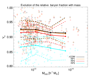
for our four fully self-consistent simulations. We plot in Fig. 18 as a function of halo virial mass the relative baryon fraction defined as:

$$Y_{b}\equiv\frac{f_{b}}{\Omega_{b}/\Omega_{m}}\,.$$ (48)

For the $\Lambda$CDM case, our results for the evolution of $Y_{b}$ are consistent with the value of $Y_{b}\sim 0.92$ found by the Santa Barbara Cluster Comparison Project (Frenk et al., 1999), and with the more recent results of Ettori et al. (2006) and Gottloeber & Yepes (2007), while for the coupled models the relative baryon fraction shows a progressive decrease with increasing coupling, down to a value of $Y_{b}\sim 0.86-0.87$ for the RP5 case.

Figure 18: Evolution with virial mass $M_{200}$ of the relative baryon fraction $Y_{b}$ within the virial radius $r_{200}$ of all the halos in our sample. The coloured diamonds represent the relative baryon fraction of each single halo, while the filled circles and the coloured curves show the behaviour of the mean relative baryon fraction in each mass bin for the four fully self-consistent high-resolution simulations. A decrease of $Y_{b}$ with increasing coupling is clearly visible both in the distribution of the individual halos and in the averaged curves.

It is also important to notice that this effect is always towards lower baryon fractions in clusters with respect to the cosmological value. This could in fact alleviate tensions between the high baryon abundance estimated from CMB observations, and the somewhat lower values inferred from detailed X-ray observations of galaxy clusters (Vikhlinin et al., 2006; McCarthy et al., 2007; LaRoque et al., 2006; Afshordi et al., 2007).

5 Conclusions

We have investigated coupled DE cosmologies, both with respect to their expected background and linear perturbation evolution, as well as in their predictions for the nonlinear regime of structure formation. To do so we have developed and tested in this work a modified version of the cosmological N-body code GADGET-2 suitable for evolving these kinds of cosmological models. The numerical implementation we have developed is in fact quite general and not restricted to the simple specific models of coupled quintessence that we have investigated in this paper. Instead, it should be well suited for a much wider range of DE models. We also note that the ability to selectively enable or disable each of the modifications discussed above, makes the code suitable for cosmological models that are unrelated to the coupled DE scenario but require similar new degrees of freedom that our implementation allows. These are:

1. the expansion history of the Universe can be specified according to any desired evolution of the Hubble rate as a function of the scale factor $a$;

2. a global variation in time of the gravitational constant and/or a variation in time of the gravitational strength for each individual matter species. This includes the possibility to have a long range repulsive interaction between different particle species;

3. variation in time of the particle mass of each individual matter species;

4. extra velocity-dependent terms in the equation of motion for each individual matter species.

With this implementation we have investigated the effects of coupled DE models with a constant coupling $\beta_{c}$ to the CDM fluid on structure formation. We have shown that the halo mass function is modified in coupled DE models, but can still be well fitted at different redshifts by the Jenkins et al. (Jenkins et al., 2001) fitting formula, or by the Sheth & Tormen (Sheth & Tormen, 1999) formula, which yields a moderately better agreement, especially at $z>0$.

We have confirmed the analytic prediction that density fluctuations in baryons and CDM will develop a bias on all scales due to the presence of a fifth-force acting only between CDM particles. We have also shown that in addition to this the bias is enhanced when moving from the linear regime of very large scales to smaller and progressively more non-linear scales.

We have investigated the evolution of the bias between baryons and CDM overdensities down to the very nonlinear regime found in the inner part of collapsed objects, in the same fashion as described in Macciò et al. (2004). We found here similar results with this previous work, namely an enhancement of the bias in the nonlinear region within and around massive halos. We also recover from this analysis the large scale value of the linear bias computed from the power spectrum when integrating the bias function up to very large radii from the centre of CDM halos. The enhancement of the bias in highly nonlinear structures has an impact on the determination of the baryon fraction from cluster measurements, and we have computed for all our halos, without including non-adiabatic processes, the evolution of this fraction within the virial radius $r_{200}$ with coupling, finding that the baryon fraction is reduced with increasing coupling by up to $\sim 8-10\%$ with respect to $\Lambda$CDM for the largest coupling value.

We have also investigated the effect of the coupling on the halo density profiles. We find that they are remarkably well fit over the resolved range by the NFW formula for any value of the coupling. There is a clear trend of a decrease of the inner halo overdensity with respect to $\Lambda$CDM with increasing coupling (or, equivalently, an increase of the scale radius $r_{s}$ for increasing coupling). This result conflicts with previous claims for the same class of coupled DE models (Macciò et al., 2004).

Using a number of special test simulations, we have identified the origin of this effect of reduced halo concentrations for increasing coupling. It actually arises from a combination of two peculiar features that the coupling introduces in the Newtonian limit of gravitational dynamics. The first of these is the decrease of CDM particle mass with time, which causes the total potential energy of a halo to decrease, and hence effectively moves the system to a configuration where an excess of kinetic energy is present relative to virial equilibrium. The second one is the additional velocity-dependent term, which directly raises the total kinetic energy density of halos by accelerating their particles in the direction of their peculiar velocity. Both of these effects cause a halo to slightly expand in order to restore virial equilibrium, and this reduces the halo concentration.

In conclusion, we have developed a general numerical implementation of coupled dark energy models in the GADGET-2 code. We have then performed the first fully self-consistent high-resolution hydrodynamic N-body simulations of interacting dark energy models with constant coupling, and carried out a basic analysis of the non-linear structures that formed. Interestingly, we found that a larger coupling leads to a lower average halo concentration. Furthermore, both the baryon fraction in massive halos and the inner overdensity of CDM halos decrease with increasing coupling. These effects alleviate the present tensions between observations and the $\Lambda$CDM model on small scales, implying that the coupled DE models are viable alternatives to the cosmological constant included in standard $\Lambda$CDM.

References

- Afshordi et al. (2007) Afshordi N., Lin Y.-T., Nagai D., Sanderson A. J. R., 2007, Mon. Not. Roy. Astron. Soc., 378, 293
- Allen et al. (2004) Allen S. W., Schmidt R. W., Ebeling H., Fabian A. C., van Speybroeck L., 2004, Mon. Not. Roy. Astron. Soc., 353, 457
- Amendola (2000) Amendola L., 2000, Phys. Rev., D62, 043511
- Amendola (2004) Amendola L., 2004, Phys. Rev., D69, 103524
- Amendola et al. (2008) Amendola L., Baldi M., Wetterich C., 2008, Phys. Rev., D78, 023015
- Amendola & Quercellini (2004) Amendola L., Quercellini C., 2004, Phys. Rev. Lett., 92, 181102
- Anderson & Carroll (1997) Anderson G. W., Carroll S. M., 1997
- Astier et al. (2006) Astier P., et al., 2006, Astron. Astrophys., 447, 31
- Baldi & Macciò (in prep.) Baldi M., Macciò A. V., in prep.
- Bardeen et al. (1986) Bardeen J. M., Bond J. R., Kaiser N., Szalay A. S., 1986, Astrophys. J., 304, 15
- Bean et al. (2008) Bean R., Flanagan E. E., Laszlo I., Trodden M., 2008
- Bertolami et al. (2007) Bertolami O., Gil Pedro F., Le Delliou M., 2007, Phys. Lett., B654, 165
- Binney & Evans (2001) Binney J. J., Evans N. W., 2001, Mon. Not. Roy. Astron. Soc., 327, L27
- Brookfield et al. (2008) Brookfield A. W., van de Bruck C., Hall L. M. H., 2008, Phys. Rev., D77, 043006
- Damour et al. (1990) Damour T., Gibbons G. W., Gundlach C., 1990, Phys. Rev. Lett., 64, 123
- Di Porto & Amendola (2008) Di Porto C., Amendola L., 2008, Phys. Rev., D77, 083508
- Doran (2005) Doran M., 2005, JCAP, 0510, 011
- Doran & Robbers (2006) Doran M., Robbers G., 2006, JCAP, 0606, 026
- Doran et al. (2001) Doran M., Schwindt J.-M., Wetterich C., 2001, Phys. Rev., D64, 123520
- Eisenstein & Hu (1998) Eisenstein D. J., Hu W., 1998, Astrophys. J., 496, 605
- Ettori et al. (2006) Ettori S., Dolag K., Borgani S., Murante G., 2006, Mon. Not. Roy. Astron. Soc., 365, 1021
- Farrar & Peebles (2004) Farrar G. R., Peebles P. J. E., 2004, ApJ, 604, 1
- Farrar & Rosen (2007) Farrar G. R., Rosen R. A., 2007, Physical Review Letters, 98, 17, 171302
- Flores & Primack (1994) Flores R. A., Primack J. R., 1994, Astrophys. J., 427, L1
- Francis et al. (2008a) Francis M. J., Lewis G. F., Linder E. V., 2008a
- Francis et al. (2008b) Francis M. J., Lewis G. F., Linder E. V., 2008b
- Frenk et al. (1999) Frenk C. S., White S. D. M., Bode P., et al., 1999, ApJ, 525, 554
- Gottloeber & Yepes (2007) Gottloeber S., Yepes G., 2007, Astrophys. J., 664, 117
- Gromov et al. (2004) Gromov A., Baryshev Y., Teerikorpi P., 2004, Astron. Astrophys., 415, 813
- Grossi & Springel (2008) Grossi M., Springel V., 2008
- Gubser & Peebles (2004) Gubser S. S., Peebles P. J. E., 2004, Phys. Rev. D, 70, 12, 123511
- Guo et al. (2007) Guo Z.-K., Ohta N., Tsujikawa S., 2007, Phys. Rev., D76, 023508
- Huey & Wandelt (2006) Huey G., Wandelt B. D., 2006, Phys. Rev., D74, 023519
- Jenkins et al. (2001) Jenkins A., et al., 2001, Mon. Not. Roy. Astron. Soc., 321, 372
- Kesden & Kamionkowski (2006) Kesden M., Kamionkowski M., 2006, Phys. Rev., D74, 083007
- Keselman et al. (2009) Keselman J. A., Nusser A., Peebles P. J. E., 2009
- Kodama & Sasaki (1984) Kodama H., Sasaki M., 1984, Prog. Theor. Phys. Suppl., 78, 1
- Komatsu et al. (2008) Komatsu E., et al., 2008
- La Vacca et al. (2009) La Vacca G., Kristiansen J. R., Colombo L. P. L., Mainini R., Bonometto S. A., 2009, JCAP, 0904, 007
- LaRoque et al. (2006) LaRoque S., et al., 2006, Astrophys. J., 652, 917
- Laszlo & Bean (2008) Laszlo I., Bean R., 2008, Phys. Rev., D77, 024048
- Lee et al. (2006) Lee S., Liu G.-C., Ng K.-W., 2006, Phys. Rev., D73, 083516
- Ma & Bertschinger (1995) Ma C.-P., Bertschinger E., 1995, Astrophys. J., 455, 7
- Macciò et al. (2004) Macciò A. V., Quercellini C., Mainini R., Amendola L., Bonometto S. A., 2004, Phys. Rev., D69, 123516
- Mainini (2005) Mainini R., 2005, Phys. Rev., D72, 083514
- Mainini & Bonometto (2006) Mainini R., Bonometto S., 2006, Phys. Rev., D74, 043504
- Mainini & Bonometto (2007a) Mainini R., Bonometto S., 2007a, JCAP, 0706, 020
- Mainini & Bonometto (2007b) Mainini R., Bonometto S., 2007b, JCAP, 0706, 020
- Manera & Mota (2006) Manera M., Mota D. F., 2006, Mon. Not. Roy. Astron. Soc., 371, 1373
- Mangano et al. (2003) Mangano G., Miele G., Pettorino V., 2003, Mod. Phys. Lett., A18, 831
- Matarrese et al. (2003) Matarrese S., Pietroni M., Schimd C., 2003, JCAP, 0308, 005
- McCarthy et al. (2007) McCarthy I. G., Bower R. G., Balogh M. L., 2007, Mon. Not. Roy. Astron. Soc., 377, 1457
- Moore (1994) Moore B., 1994, Nature, 370, 629
- Navarro et al. (1996) Navarro J. F., Frenk C. S., White S. D. M., 1996, Astrophys. J., 462, 563
- Navarro et al. (1997) Navarro J. F., Frenk C. S., White S. D. M., 1997, Astrophys. J., 490, 493
- Navarro & Steinmetz (2000) Navarro J. F., Steinmetz M., 2000, Astrophys. J., 528, 607
- Neto et al. (2007) Neto A. F., et al., 2007
- Newman et al. (2009) Newman A. B., et al., 2009
- Nusser et al. (2005) Nusser A., Gubser S. S., Peebles P. J. E., 2005, Phys. Rev., D71, 083505
- Oyaizu (2008) Oyaizu H., 2008
- Peebles (1980) Peebles P. J. E., 1980, The Large-Scale Structure of the Universe, Princeton University Press
- Percival et al. (2001) Percival W. J., et al., 2001, Mon. Not. Roy. Astron. Soc., 327, 1297
- Perlmutter et al. (1999) Perlmutter S., et al., 1999, Astrophys. J., 517, 565
- Pettorino & Baccigalupi (2008) Pettorino V., Baccigalupi C., 2008, Phys. Rev., D77, 103003
- Quartin et al. (2008) Quartin M., Calvao M. O., Joras S. E., Reis R. R. R., Waga I., 2008, JCAP, 0805, 007
- Ratra & Peebles (1988) Ratra B., Peebles P. J. E., 1988, Phys. Rev., D37, 3406
- Riess et al. (1998) Riess A. G., et al., 1998, Astron. J., 116, 1009
- Sand et al. (2002) Sand D. J., Treu T., Ellis R. S., 2002, Astrophys. J., 574, L129
- Sand et al. (2004) Sand D. J., Treu T., Smith G. P., Ellis R. S., 2004, Astrophys. J., 604, 88
- Sheth & Tormen (1999) Sheth R. K., Tormen G., 1999, Mon. Not. Roy. Astron. Soc., 308, 119
- Simon et al. (2003) Simon J. D., Bolatto A. D., Leroy A., Blitz L., 2003, Astrophys. J., 596, 957
- Springel (2005) Springel V., 2005, Mon. Not. Roy. Astron. Soc., 364, 1105
- Springel & Farrar (2007) Springel V., Farrar G. R., 2007, MNRAS, 380, 911
- Springel et al. (2008) Springel V., Wang J., Vogelsberger M., et al., 2008, MNRAS, 391, 1685
- Springel et al. (2001) Springel V., White S. D. M., Tormen G., Kauffmann G., 2001, MNRAS, 328, 726
- Stabenau & Jain (2006) Stabenau H. F., Jain B., 2006, Phys. Rev., D74, 084007
- Sutter & Ricker (2008) Sutter P. M., Ricker P. M., 2008
- Vikhlinin et al. (2006) Vikhlinin A., et al., 2006, Astrophys. J., 640, 691
- Wang et al. (2007) Wang B., Zang J., Lin C.-Y., Abdalla E., Micheletti S., 2007, Nucl. Phys., B778, 69
- Wetterich (1988) Wetterich C., 1988, Nucl. Phys., B302, 668
- Wetterich (1995) Wetterich C., 1995, Astron. Astrophys., 301, 321
- Zel’dovich (1970) Zel’dovich Y. B., 1970, Astron. Astrophys., 5, 84