Early time kinetics of systems with spatial symmetry breaking

Abstract

In this paper we present a study of the early stages of unstable state evolution of systems with spatial symmetry changes. In contrast to the early time linear theory of unstable evolution described by Cahn, Hilliard, and Cook, we develop a generalized theory that predicts two distinct stages of the early evolution for symmetry breaking phase transitions. In the first stage the dynamics is dominated by symmetry preserving evolution. In the second stage, which shares some characteristics with the Cahn-Hilliard-Cook theory, noise driven fluctuations break the symmetry of the initial phase on a time scale which is large compared to the first stage for systems with long interaction ranges. To test the theory we present the results of numerical simulations of the initial evolution of a long-range antiferromagnetic Ising model quenched into an unstable region. We investigate two types of symmetry breaking transitions in this system: disorder-to-order and order-to-order transitions. For the order-to-order case, the Fourier modes evolve as a linear combination of exponentially growing or decaying terms with different time scales.

I introduction

Many systems have effective long-range interactions and exhibit a variety of crystalline phases. Some examples are metals (Christian2002, ), block copolymers (Bates and Fredrickson, 1990), and systems with modulated phases (Seul and Andelman, 1995; Garel and Doniach, 1982; Lacoste and Lubensky, 2001). The kinetics of the transitions from a disordered, spatially uniform state to a spatially periodic state (disorder-to-order) have been explored in several contexts (see, for example, Refs. (Harrison et al., 2000; Roland and Desai, 1990; Wickham et al., 2003; Fredrickson and Binder, 1989).) Some aspects of the kinetics from one spatially periodic state to another (order-to-order) have also been investigated (Li2007a, ; Li et al., 2007; Yu et al., 2005; Nonomura and Ohta, 2001).

For systems with long-range interactions the phase ordering process is separated into an early time regime described by a linear theory, an intermediate regime where nonlinear effects first become important, and a late stage domain coarsening regime. Phase ordering, a process whereby a disordered state evolves into a state with macroscopic regions of like components, has been well studied for systems described by a Landau-Ginzburg free energy, such as the ferromagnetic Ising model (Gunton et al., 1983). If the coarse-grained order parameter is locally conserved, the phase ordering process is called spinodal decomposition. If it is not conserved, the process is called continuous ordering. The latter case is referred to as Model A and the former is referred to as Model B (Hohenberg and Halperin, 1977).

“Phase ordering” as used here is distinct from a disorder-to-order transition, which we take to mean a transition from a disordered to a spatially periodic state. A disorder-to-order transition breaks spatial symmetry; that is, the initial state has a spatial symmetry that is absent in the final state. In contrast, phase ordering for the ferromagnetic Ising model with a non-conserved order parameter has uniform spatial symmetry in both the initial and final phases. Thus, in this case phase ordering does not break spatial symmetry symmetry .

The early time linear regime of phase ordering was first studied by Cahn and Hilliard (Cahn and Hilliard, 1958, 1959; Cahn1967, ) and later by Cook (Cook1970, ). The early time theory was extended to the intermediate time regime by Langer, Bar-on, and Miller (Langer et al., 1975) for Model B and by Billotet and Binder (Billotet and Binder, 1979) for Model A. The Lifshitz-Slyozov theory (Lifshitz, 1961) describes the late time regime for Model B which is dominated by the surface tension of domain walls. The theory of late stage boundary motion for model A was developed by Allen and Cahn (ALLEN1979, ).

The Cahn, Hilliard, and Cook (CHC) linear theory was originally developed to describe spinodal decomposition for systems such as binary alloys, where the order parameter is locally conserved. The CHC theory predicts exponential growth of certain Fourier modes immediately after a temperature quench into the unstable regime (Cahn and Hilliard, 1958, 1959; Cahn1967, ; Cook1970, ). For systems with long-range interactions, this exponential growth lasts for a time proportional to the logarithm of the interaction range (Binder, 1984).

CHC theory also describes continuous ordering for systems such as the ferromagnetic Ising model, with a non-conserved order parameter. In this case the temperature is quenched to below the critical temperature at zero external field (a critical quench). However, if the external field is non-zero during the temperature quench (an off-critical quench), CHC theory is not applicable. We will show that CHC theory also fails to describe a wide class of transitions that break spatial symmetry.

In this paper we extend the CHC theory to describe transitions that break spatial symmetry and whose dynamics do not conserve the order parameter analogy . For these systems we find two distinct stages of the early time evolution in contrast to CHC. Stage one, which is absent in CHC theory, is dominated by symmetry preserving dynamics. The time scale for which this stage applies is independent of the interaction range. Stage two is analogous to the early time evolution described by CHC because the dynamical equations are characterized by exponential solutions, and the time scale for which stage two is valid is longer for longer interaction ranges. For disorder-to-order transitions certain Fourier modes grow exponentially. In contrast, for order-to-order transitions the Fourier modes evolve as a linear combination of exponentially growing or decaying terms with different time scales.

Our particular system of interest is the long-range antiferromagnetic Ising model. This system has spatial symmetry breaking disorder-to-order and order-to-order transitions. We use Monte Carlo techniques to simulate the system and compare our results to our numerical solutions of a Langevin equation and to our analytical predictions.

The structure of the paper is as follows. Section II summarizes the theoretical background on unstable state evolution for models described by a Landau-Ginzburg free energy, focusing on the linear CHC theory. We extend this theory to include symmetry breaking transitions in Sec. III. The role that symmetry breaking plays in the interplay between the two stages is discussed. The long-range antiferromagnetic Ising model and its phase diagram are introduced in Sec. IV. We develop the generalized theory for this model by using the Langevin equation based on a coarse-grained free energy as well as the Langevin equation describing Glauber dynamics. Our numerical and theoretical results are presented for the disorder-to-order case in Sec. V and for the order-to-order case in Sec. VI. Section VII summarizes and discusses our results.

II review of CHC theory for continuous ordering

In this section we review the Cahn-Hilliard-Cook (CHC) theory as it is applied to continuous ordering for which the order parameter is not conserved. We begin with the Langevin equation for the evolution of the order parameter $\hat{\phi}(\boldsymbol{x},t)$:

$$\frac{\partial\hat{\phi}(\boldsymbol{x},t)}{\partial t}=-M\left(\frac{\delta F[\hat{\phi}]}{\delta\hat{\phi}(\boldsymbol{x})}\right)+\sqrt{B}\eta(\boldsymbol{x},t),$$ (1)

where $F$ is the coarse grained free energy, and $M$ is the mobility (which for the CHC theory is assumed to be a constant in space and time) and

$$B=2MT$$ (2)

from the fluctuation dissipation relationship where we have set $k_{B}=1$. Equation (1) is also known as the time-dependent Ginzburg-Landau equation (Bray1995, ). The first term on the right-hand side of Eq. (1), which we call the drift term, lowers the free energy as time evolves. The second term describes the noise and represents the small scale fast dynamics as random forces. We will take the noise to be white Gaussian and to obey the conditions:

$$\left\langle\eta(\boldsymbol{x},t)\right\rangle =0$$ (3)

$$\left\langle\eta(\boldsymbol{x},t)\eta(\boldsymbol{x^{\prime}},t^{\prime})\right\rangle =\delta(\boldsymbol{x}-\boldsymbol{x^{\prime}})\delta(t-t^{\prime}).$$ (4)

By using the the Landau-Ginzburg free energy,

$$F[\hat{\phi}(\boldsymbol{x})] =\!\int\!d\boldsymbol{x}\Big{(}\frac{R^{2}}{2}[\nabla\hat{\phi}(\boldsymbol{x})]^{2}+\frac{\epsilon}{2}\hat{\phi}^{2}(\boldsymbol{x})$$

$$\quad+\frac{1}{4}\hat{\phi}^{4}(\boldsymbol{x})-h\hat{\phi}(\boldsymbol{x})\Big{)},$$ (5)

Eq. (1) becomes,

$$\frac{\partial\hat{\phi}(\boldsymbol{x},t)}{\partial t} = -M\{-R^{2}\nabla^{2}\hat{\phi}(\boldsymbol{x},t)+\epsilon\hat{\phi}(\boldsymbol{x},t)$$ (6)

$${}+\hat{\phi}^{3}(\boldsymbol{x},t)-h\}+\sqrt{B}\eta(\boldsymbol{x},t),$$

where $\epsilon=(T-T_{c})/T_{c}$ is the reduced temperature, $T_{c}$ is the critical temperature, $h$ is the external field, and $R$ is the interaction range. The extrema of the free energy can be found by solving the Euler-Lagrange equation:

$$0 =\frac{\delta F[\hat{\phi}]}{\delta\hat{\phi}(\boldsymbol{x})}$$

$$=-R^{2}\nabla^{2}\hat{\phi}(\boldsymbol{x},t)+\epsilon\hat{\phi}(\boldsymbol{x},t)+\hat{\phi}^{3}(\boldsymbol{x},t)-h.$$ (7)

For a critical quench the initial state is equilibrated at initial temperature $T_{i}>T_{c}$ in zero external field $h_{i}=0$. The temperature is instantaneously quenched to a final temperature $T_{f}<T_{c}$ in the unstable regime where $\epsilon_{f}=(T_{f}-T_{c})/T_{c}<0$, keeping the external field $h_{f}=0$. Before the quench, the system is in a disordered state corresponding to the average order parameter, $\hat{\phi}_{0}=\langle\hat{\phi}(\boldsymbol{x})\rangle=0$ for spatially homogeneous systems. We will consider small fluctuations, $\hat{\psi}(\boldsymbol{x},t)$, of the order parameter about this value, $\hat{\phi}(\boldsymbol{x},t)=\hat{\phi}_{0}+\hat{\psi}(\boldsymbol{x},t)=\hat{\psi}(\boldsymbol{x},t),$ and keep terms first order in $\hat{\psi}(\boldsymbol{x},t)$ so that Eq. (6) becomes:

$$\frac{\partial\hat{\psi}(\boldsymbol{x},t)}{\partial t} =-M\left(-R^{2}\nabla^{2}\hat{\psi}(\boldsymbol{x},t)-|\epsilon_{f}|\hat{\psi}(\boldsymbol{x},t)\right)$$

$$\qquad+\sqrt{B}\eta(\boldsymbol{x},t).$$ (8)

We have used the fact that $\hat{\phi}_{0}=0$ is a solution to Eq. (7). In Fourier space Eq. (8) becomes

$$\frac{\partial\hat{\psi}(\boldsymbol{k},t)}{\partial t}=D_{\rm chc}(k)\hat{\psi}(\boldsymbol{k},t)+\sqrt{B}\eta(\boldsymbol{k},t),$$ (9)

with

$$D_{\rm chc}(k)=-M(R^{2}k^{2}-|\epsilon_{f}|).$$ (10)

We see from Eq. (9) that the individual Fourier modes evolve independently of one another. The solution to Eq. (9) is

$$\hat{\psi}(\boldsymbol{k},t) = \hat{\psi}(\boldsymbol{k},0)\exp\left(D_{\rm chc}(k)t\right)$$ (11)

$${}+\sqrt{B}\!\int_{0}^{t}\eta(\boldsymbol{k},t)G(t-t^{\prime})dt^{\prime},$$

where $G(t-t^{\prime})=\exp((t-t^{\prime})D_{\rm chc}(k))$. We use the definition of the equal time structure factor $S(\boldsymbol{k},t)=\left\langle\phi(\boldsymbol{k},t)\phi(-\boldsymbol{k},t)\right\rangle/V,$ Eq. (2), and the properties of the noise (Eqs. (3) and (4)) to obtain:

$$S(k,t) = e^{2D_{\rm chc}(k)t}\left(S(k,t=0)+\frac{M}{\beta_{f}D_{\rm chc}(k)}\right)$$ (12)

$${}-\frac{M}{\beta_{f}D_{\rm chc}(k)},$$

where $\beta_{f}=T_{f}^{-1}$.

Systems with $R\gg 1$ are said to be near-mean-field and the limit $R\rightarrow\infty$ is the mean-field limit (klein2007, ). For $T_{f}<T_{c}$ simulations have shown that Eq. (12) is applicable for systems with $R\gg 1$ for some initial time after the quench (Heermann, 1984, 1985; Izumitani and Hashimoto, 1985; Okada and Han, 1986). Binder (Binder, 1984) has argued that the linear theory should break down when the fluctuations are large in comparison to the average order parameter. He predicted that CHC theory breaks down at a time $\tau$ that scales as $\tau\sim\ln{R}$ (see Eq. (18)).

To understand Binder’s result, we consider how $\hat{\psi}(\boldsymbol{k})$ depends explicitly on $R$, the relevant length scale of the problem. We scale all lengths with $R$ by defining $\boldsymbol{r\equiv\boldsymbol{x}}/R,$ and $\boldsymbol{q}\equiv\boldsymbol{k}R.$ We see from Eq. (10) that $D_{\rm chc}(q)$ is independent of $R$. It follows that $G(t-t^{\prime})$ is also independent of $R$, and from Eq. (11) $\hat{\psi}(\boldsymbol{k},t)$, $\hat{\psi}(\boldsymbol{k},0)$, and $\eta(\boldsymbol{k},t)$ must depend explicitly on $R$ in the same way. Equations (3) and (4) become

$$\left\langle\eta(\boldsymbol{r},t)\right\rangle =0$$ (13)

$$\left\langle\eta(\boldsymbol{r},t)\eta(\boldsymbol{r^{\prime}},t^{\prime})\right\rangle =\delta(\boldsymbol{r}-\boldsymbol{r^{\prime}})\delta(t-t^{\prime}).$$ (14)

From Eq. (14) and $\delta(\boldsymbol{x})=R^{-d}\delta(\boldsymbol{r})$ the noise must satisfy $\eta(\boldsymbol{x},t)=R^{-d/2}\eta(\boldsymbol{r},t)$, or

$$\eta(\boldsymbol{k},t)=R^{-d/2}\eta(\boldsymbol{q},t),$$ (15)

where $\eta(\boldsymbol{q},t)=\int d\boldsymbol{x}\,\rm{e}^{-i\boldsymbol{k}\cdot\boldsymbol{x}}\,\eta(\boldsymbol{r},t).$ This motivates us to introduce $\psi(\boldsymbol{q},t)$ through

$$\hat{\psi}(\boldsymbol{k},t)=R^{-d/2}\psi(\boldsymbol{q},t).$$ (16)

and $\psi(\boldsymbol{r},t)$ though $\psi(\boldsymbol{q},t)=\int d\boldsymbol{x}\,\rm{e}^{-i\boldsymbol{k}\cdot\boldsymbol{x}}\,\psi(\boldsymbol{r},t)$ and is independent of $R$. We consider the dynamics of $\psi(\boldsymbol{r}).$ If we substitute Eqs. (15) and (16) into Eq. (8) and use a Laplacian with respect to scaled coordinates $\nabla^{2}_{r}=R^{2}\nabla^{2}$ all $R$ dependence in Eq. (8) cancels. Thus the solution to Eq. (8), $\psi(\boldsymbol{r},t)$, is also independent of $R.$ Equations (15) and (16) mean that larger $R$ results in effectively smaller noise and noise induced fluctuations.

We may drop the $\hat{\psi}^{3}(\boldsymbol{x})$ term in Eq. (8) only if $\hat{\psi}(\boldsymbol{x})\gg\hat{\psi}^{3}(\boldsymbol{x})$. Thus we estimate the breakdown time $\tau$ from the condition $\hat{\psi}^{2}(\boldsymbol{x})\sim 1$. For a given value of $q$ this condition gives

$$\frac{\exp\left(2D(q)\tau\right)}{R^{d}}\sim 1,$$ (17)

which yields

$$\tau\sim\frac{d\ln R}{2D(q)}.$$ (18)

where we have used Eq. (16) along with the time dependence of Eq. (11). Note that the result for the breakdown of the linear theory is a consistency argument, and it is possible for the linear theory to fail earlier than the time given in Eq. (18).

The result that the duration of applicability of the linear theory is longer for larger $R$ is illuminated by a simple mechanical analogy (see Fig. 1). The CHC theory describes the evolution of certain fluctuations of the system about an unstable stationary point of the free energy. The system is analogous to a ball sitting at the top of a fairly flat hill subject to small random perturbations. These perturbations will eventually cause the ball to roll off the hill; the smaller the perturbations, the longer it takes for the ball to roll off. As $R$ increases the noise effectively decreases and the system remains near the unstable point of the free energy longer. When the free energy can no longer be approximated quadratically, the CHC theory is no longer valid.

III Generalization of CHC theory

Equation (1) is an example of a dissipative Langevin equation. Because we will also consider Glauber dynamics, we consider a Langevin equation of the more general form,

$$\frac{\partial\phi(\boldsymbol{r},t)}{\partial t}=\Theta[\phi,\boldsymbol{r}]+\sqrt{B[\phi,\boldsymbol{r}]}R^{-d/2}\eta(\boldsymbol{r},t),$$ (19)

where $\phi(\boldsymbol{r},t)$ is the order parameter with scaled coordinates, the drift term $\Theta[\phi,\boldsymbol{r}]$ is nonlinear in $\phi(\boldsymbol{r},t)$ and the noise satisfies Eqs. (13) and (14). Equation (19) is written in scaled coordinates so that the $R$-dependence of the noise term is explicit ($\Theta[\phi,\boldsymbol{r}]$ and $B[\phi,\boldsymbol{r}]$ are independent of $R$.)

In Sec. II we derived the CHC theory as an expansion about a uniform order parameter background. This background configuration was the solution to the Euler-Lagrange equation for the parameters both before and after the quench and is therefore time independent after a critical quench. More generally, we will expand about a background configuration $\phi_{b}(\boldsymbol{r},t)$ which is not necessarily uniform and may be time dependent after the quench.

At the time of the quench, the system is in a configuration consistent with the equilibrium state before the quench. We can write this state as $\phi(\boldsymbol{r},t=0)=\phi_{b}(\boldsymbol{r},t=0)+R^{-d/2}\psi(\boldsymbol{r},t=0).$ The background configuration $\phi_{b}(\boldsymbol{r},t=0)$ is a solution to the Euler-Lagrange equation for $T_{i}$ and $h_{i}$, is independent of the noise, and may be nonuniform. The term $R^{-d/2}\psi(\boldsymbol{r},t=0)$ represents small fluctuations about the background due to the noise. In general, $\phi_{b}(\boldsymbol{r},t=0)\neq\phi_{0}(\boldsymbol{r});$ that is, the background configuration is not a stationary point of the free energy and may be time dependent after the quench. We are interested in how this background configuration and these fluctuations evolve with time after the quench, that is the time evolution of

$$\phi(\boldsymbol{r},t)=\phi_{b}(\boldsymbol{r},t)+R^{-d/2}\psi(\boldsymbol{r},t).$$ (20)

If we expand Eq. (19) to first order in the small fluctuations, $R^{-d/2}\psi(\boldsymbol{r},t)$, about the background configuration $\phi_{b}(\boldsymbol{r},t)$, we obtain

$$\frac{\partial\phi_{b}(\boldsymbol{r},t)}{\partial t}+R^{-d/2}\frac{\partial\psi(\boldsymbol{r},t)}{\partial t}=\Theta[\phi,\boldsymbol{r}]|_{\phi=\phi_{b}}$$

$$\quad+\!\int\!d\boldsymbol{r}^{\prime}\frac{\delta\Theta[\phi,\boldsymbol{r}]}{\delta\phi(\boldsymbol{r}^{\prime},t)}\Big{|}_{\phi=\phi_{b}}R^{-d/2}\psi(\boldsymbol{r}^{\prime},t)$$

$$\quad+\sqrt{B[\phi,\boldsymbol{r}]}\Big{|}_{\phi=\phi_{b}}R^{-\mbox{}d/2}\eta(\boldsymbol{r},t).$$ (21)

It is natural to separate Eq. (21) terms of order $R^{0}$ from terms of order $R^{-d/2}$ giving the dynamical equations for the background and the fluctuations. The equation for the evolution of the background configuration, which is zeroth order in $R^{-d/2}$, is

$$\frac{\partial\phi_{b}(\boldsymbol{r},t)}{\partial t}=\Theta[\phi]|_{\phi=\phi_{b}}.\hskip 5.69046pt\mbox{(evolution of background)}$$ (22)

Equation (22) is noiseless and independent of $R$. In contrast, the equation for the evolution of the fluctuations is noise driven and is first order in $R^{-d/2}$:

$$\frac{\partial\psi(\boldsymbol{r},t)}{\partial t} = \!\int\!d\boldsymbol{r}^{\prime}\frac{\delta\Theta[\phi,\boldsymbol{r}]}{\delta\phi(\boldsymbol{r}^{\prime},t)}\Big{|}_{\phi=\phi_{b}}\psi(\boldsymbol{r}^{\prime},t)$$ (23)

$${}+\sqrt{B[\phi]}\mid_{\phi=\phi_{b}}\eta(\boldsymbol{r},t).$$

(evolution of fluctuations)

The background configuration $\phi_{b}(\boldsymbol{r},t)$ and the fluctuations $\psi(\boldsymbol{r},t)$ evolve simultaneously; Eqs. (22) and (23) together describe the early time kinetics of unstable systems. Equation (23) differs from the CHC theory described in Sec. II because the coefficient of $\psi(\boldsymbol{r},t)$ on the right-hand side of Eq. (23) depends on $\phi_{b}(\boldsymbol{r},t)$, which evolves according to Eq. (22). Because of the explicit time dependence of $\phi_{b}(\boldsymbol{r},t)$, we do not expect to find exponential solutions as found in the CHC theory.

Equation (22) dominates the evolution of $\phi(\boldsymbol{r},t)$ until $\big{|}\Theta[\phi]|_{\phi=\phi_{b}}\big{|}\sim R^{-d/2}$ (we will discuss specific examples of this evolution in the following). We refer to the kinetics while the background configuration is evolving as stage one. If

$$\big{|}\Theta[\phi]|_{\phi=\phi_{b}}\big{|}\ll R^{-d/2},$$ (24)

we refer to the kinetics as stage two.

If $\Theta[\phi]\propto\delta F/\delta\phi$, then Eq. (19) becomes a dissipative Langevin equation. In the limit $R\rightarrow\infty$ the condition for stage two evolution (Eq. (24)) implies that $\delta F/\delta\phi\simeq 0$, or

$$\phi_{b}(\boldsymbol{r},t)=\phi_{0}(\boldsymbol{r}),$$ (25)

where $\phi_{0}(\boldsymbol{r})$ is an unstable solution to the Euler-Lagrange equation for the final parameters $T_{f}$ and $h_{f}$ corresponding to the temperature and external field after the quench, respectively. In stage two the dynamics shares several features with the dynamics of CHC. Namely, the background configuration is nearly a stationary point of the free energy, and the linear evolution admits (nearly) exponential solutions, which are applicable for a time $\tau\sim\ln R$, as in Eq. (18).

If $\phi_{b}(\boldsymbol{r},t=0)\neq\phi_{0}(\boldsymbol{r})$, then stage one kinetics begins immediately after the quench, and either there is no stage two kinetics at any time after the quench, or stage two kinetics follows stage one. If $\phi_{b}(\boldsymbol{r},t=0)=\phi_{0}(\boldsymbol{r})$, then stage one kinetics is absent and stage two kinetics begins immediately after the quench. Table 1 summarizes the various possibilities.

Case	Spatial symmetry breaking	Stage one	Stage two	Example
$\phi_{b}(t=0)\simeq\phi_{0}$	No	No	Yes	Critical quench for ferromagnet
	Yes	No	Yes	Critical quench for antiferromagnet
$\phi_{b}(t=0)\neq\phi_{0}$	No	Yes	No	Off-critical quench for ferromagnet
	Yes	Yes	Yes	Off-critical and external field
				quench for antiferromagnet

Table 1: Summary of early kinetics for various types of transitions for the long-range ferromagnetic Ising model and the long-range antiferromagnetic Ising model. In the table $\phi_{b}(t=0)$ is the background configuration just after the quench and $\phi_{0}$ is the unstable solution to the Euler-Lagrange equation for $T_{f}$ and $h_{i}$. These quenches are defined in the text.

A critical quench in the ferromagnetic Ising model (see Table 1 and Fig. 1(a)) exhibits stage two but not stage one kinetics. In this case $T_{i}=\infty$, $h_{i}=0$, $T_{f}<T_{c}$, $h_{f}=0$, and $\phi_{b}(t=0)=\phi_{0}$.

In contrast, an off-critical quench in the ferromagnetic Ising model (see Table 1 and Fig. 1(b)) is an example that exhibits stage one but not stage two kinetics. In the off-critical quench the initial conditions are the same as for the critical quench ($T_{i}=\infty$ and $h_{i}=0$), but the system is quenched below $T_{c}$ and $h_{f}\neq 0$. Because $h_{f}\neq 0,$ the initial background configuration $\phi_{b}(t=0)=0$ is not a solution to the Euler-Lagrange equation for the final parameters $T_{f}$ and $h_{f}$. The background configuration evolves via Eq. (22) directly toward the stable minimum $\phi_{m}$ of the free energy landscape and away from the unstable solution $\phi_{0}$ (see Fig. 1(b)). Hence, the system will never reach the unstable stationary point, and there will be no stage two kinetics.

(a)

(b)

Figure 1: A representation of the free energy landscape for a ferromagnetic Ising model as a function of the average magnetization $\langle\phi\rangle$ for (a) a critical quench and (b) an off-critical quench for $h_{f}>0.$ The dot represents the background configuration of the system immediately after the quench. For a critical quench the system is initially at an unstable stationary point of the free energy, and the CHC theory governs its early evolution. For long-range systems the noise is effectively small, and the system fluctuates about the top of the hill for an extended time. Eventually, the system will be in one of the two global minima $\phi_{m}$ if the system size and temperature are finite. For an off-critical quench the background configuration sits to the right of the free energy stationary point. The noiseless dynamics of Eq. (22) drives the system directly toward the stable minimum $\phi_{m}$ and away from the stationary point. Thus, in this case we do not expect stage two exponential growth at any time after the quench.

In contrast to the ferromagnetic Ising model note , we find stage one followed by stage two kinetics in systems that break spatial symmetry. In this case the noiseless dynamics in stage one and the initial configuration conspire to drive the configuration toward the unstable solution of the Euler-Lagrange equation $\phi_{0}$. In stage one both $\phi_{b}(\boldsymbol{r})$ and $\psi(\boldsymbol{r},t)$ evolve simultaneously until the system reaches the unstable solution $\phi_{0}$ for $T_{f}$ and $h_{f}$. Stage one kinetics is analogous to a ball rolling down a hill toward a saddle point (see Fig. 2). When the system reaches the stationary point, stage two begins. Stage two is analogous to the ball fluctuating about the top of the hill and ends when the ball finally rolls off the top of the hill towards a stable state.

Figure 2: A representation of the free energy landscape for a system with spatial symmetry breaking. For systems with short range interactions fluctuations cause the ball (representing the background configuration of the system) to roll off the hill, the ball does not approach the saddle point and stage two behavior is not observed. In contrast, for systems with long-range interactions the evolution of fluctuations governed by Eq. (23) is suppressed by a factor of $R^{-d/2},$ and the noiseless dynamics of Eq. (22) dominates. Due to this noiseless symmetry preserving dynamics the ball rolls down the hill toward the saddle point along the dashed line with little deviation due to the fluctuations. The dashed line represents all configurations with the same symmetry as the initial state. The directions perpendicular to the dashed line represent symmetry breaking degrees of freedom. Once near the saddle point, the ball essentially stops rolling (condition (24) is satisfied) and stage two kinetics takes over as unstable fluctuations grow for a time of order $\tau\sim\ln R$. Eventually, after stage two, the ball will roll off the hill along the dotted line.

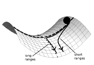
Why does the ball in Fig. 2 not roll off the hill before it reaches the saddle point? Symmetry considerations provide the answer. For dissipative dynamics where $\Theta\propto-\delta F/\delta\phi$, the noiseless dynamics of Eq. (22) preserves certain spatial symmetries, depending on the form of the free energy. The dynamics of Eq. (22) evolves $\phi_{b}(\boldsymbol{r},t)$ to the lowest free energy within these symmetry constraints. This configuration is an unstable stationary point of the free energy. It is a local minimum with respect to the symmetry constrained degrees of freedom, but a local maximum with respect to the other symmetry breaking degrees of freedom. Once at this saddle point, the nonlinear background dynamics of stage one terminates, and stage two kinetics takes over. See also Ref. (Barros2008, ).

The spatial symmetries preserved by the noiseless dynamics of Eq. (22) are not preserved by the noise driven dynamics of Eq. (23); that is, the noise causes random fluctuations which break the spatial symmetries of $\phi_{b}(\boldsymbol{r},t).$ Initially, these spatial symmetries are broken by $\psi(\boldsymbol{r},t=0),$ the fluctuations about the background at the time of the quench due to $\eta(\boldsymbol{r},t<0),$ the noise in the system before the quench. These initial fluctuations, which are of order $R^{-d/2},$ begin to grow (or decay) immediately after the quench according to Eq. (23). However, during stage one the fluctuations $\psi(\boldsymbol{r},t)$ remain of order $R^{-d/2}.$ The reason the ball in Fig. 2 does not roll off the hill is because the fluctuations which would drive the ball off the hill are small for sufficiently large $R.$ The time it takes for the ball to roll down to the saddle point (the duration of stage one), is independent of $R.$ In stage two kinetics, when the nonlinear dynamics of Eq. (22) has ceased, the symmetry breaking fluctuations continue to grow for an extended period of time, eventually becoming of the order $1.$

IV the long-range antiferromagnetic Ising model

IV.1 The model and phase diagram

To investigate a system with spatial symmetry breaking phase transitions, we simulate the long-range antiferromagnetic Ising model using Glauber Monte Carlo dynamics (Newman and Barkema, 1999). At each update a spin is selected at random and flipped with the transition probability $W=(1+\rm e^{\beta\Delta E})^{-1},$ where $\Delta E$ is the change in energy incurred from flipping the spin. Time is measured in units of Monte Carlo step per spin. For $N$ spins in a system, one Monte Carlo step (MCS) is equal to $N$ spin flip attempts. With this definition, it is natural to consider fractional Monte Carlo steps in which fewer than $N$ spin flips have been attempted.

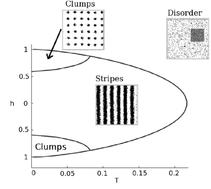
We study the two-dimensional long-range antiferromagnetic Ising model with a square shaped interaction. For this interaction a spin at $\boldsymbol{x}=(x,y)$ interacts with a second spin at $\boldsymbol{x}^{\prime}=(x^{\prime},y^{\prime})$ only if $|x-x^{\prime}|\leq R$ and $|y-y^{\prime}|\leq R$ (see Fig. 3).

There are two types of periodic low temperature configurations, which we call the stripe phase and the clump phase, that are energetically favorable with respect to the disordered phase. The system can lower its overall interaction energy in the clump or stripe phases by grouping like spins together. Although a spin pays an energy cost due to its proximity to the other spins in its own clump or stripe, it avoids interacting with most of the spins in neighboring clumps or stripes. This system is related to a previously studied model of particles (Klein et al., 1994).

An approximate phase diagram is shown in Fig. 3. The pictures are snapshots of the configurations from our Monte Carlo simulations. From Fig. 3 we see that the disorder-to-clumps transition as well as the disorder-to-stripes transition are symmetry breaking disorder-to-order transitions. In both cases the uniform spatial symmetry is lost. The two order-to-order transitions are also symmetry breaking. In the transition from stripes to clumps the continuous translational symmetry along the direction of the stripes is lost. In the clumps to stripes transition the $90^{\circ}$ rotational symmetry is lost.

The orientation of the square interaction restricts the possible alignments of the stripes and clumps: stripes must be either horizontal or vertical and clumps must be aligned in the vertical and horizontal directions. A circular-shaped potential which we do not consider here gives a honeycomb arrangement of clumps and stripes with no angular restrictions.

Figure 3: Approximate phase diagram for the long-range antiferromagnetic Ising model with a square shaped interaction. The system has two low temperature ordered phases, the clump phase and the stripe phase, and a disordered phase. The darkened square in the snapshot of the disordered Ising model shows the interaction range for a spin at the center of the square.

The Hamiltonian for the long-range antiferromagnetic Ising model is

$$H=-\frac{J}{z}\sum_{<ij>}\sigma_{i}\sigma_{j}-h\sum_{i}\sigma_{i},$$ (26)

where the brackets indicate that the summation is over all spins within the interaction range $R$, and $\sigma_{i}=\pm 1$ refers to the value of a spin at site $i$. The interaction $J=\pm 1$, where the positive sign corresponds to the ferromagnet and the negative sign corresponds to the antiferromagnet;

$$z=(2R+1)^{d}-1$$ (27)

is the number of spins within the interaction region of a single spin. Scaling the strength of the interaction by the number of the spins in an interaction range keeps the interaction energy per spin finite as we increase the $R$ (Kac et al., 1963).

IV.2 Dissipative Langevin dynamics

We now develop the equations for the relaxational Langevin dynamics as well as the background and fluctuation dynamics for a free energy which corresponds to the long-range antiferromagnetic Ising model. We begin with the coarse-grained free energy

$$F[\phi(\boldsymbol{r})] =R^{d}\Big{(}-\frac{J}{2}\!\int d\boldsymbol{r}\left((\Lambda*\phi)(\boldsymbol{r})\right)\phi(\boldsymbol{r})$$

$$\quad-\!\int d\boldsymbol{r}\left(Ts[\phi(\boldsymbol{r})]+h\phi(\boldsymbol{r})\right)\Big{)},$$ (28)

where $\phi(\boldsymbol{r})=\dfrac{1}{(\Delta)^{d}}\sum_{i}S_{i}$ is the coarse-grained magnetization of the spins inside a box of length $\Delta$ in $d$ dimensions centered at position $\boldsymbol{r}$. We use the notation $(\Lambda*\phi)(\boldsymbol{r})\equiv\!\int d\boldsymbol{r}^{\prime}\Lambda(\boldsymbol{r}-\boldsymbol{r}^{\prime})\phi(\boldsymbol{r}^{\prime})$ to denote a spatial convolution. As in Eq. (26) $J=+1$ for the ferromagnet and $J=-1$ for the antiferromagnet. The entropy density $s[\phi(\boldsymbol{r})]$ due to the coarse-graining procedure is

$$s[\phi(\boldsymbol{r})] =2\ln 2-\frac{1}{2}\{(1+\phi(\boldsymbol{r}))\ln{(1+\phi(\boldsymbol{r}))}$$

$$\qquad+(1-\phi(\boldsymbol{r}))\ln{(1-\phi(\boldsymbol{r}))}\}.$$ (29)

The scaling of the strength of the interaction is implicit in the interaction function $\Lambda(\boldsymbol{r})$ which we take to be a repulsive pairwise step potential of the form

$$\Lambda(x,y)=\begin{cases}1/z&(-R\leq x,y\leq R)\\ 0&\textnormal{otherwise}\end{cases},$$ (30)

where $z\sim(2R)^{d}$ for large $R$ (from Eq. (27)). This Kac form of the potential (Kac et al., 1963) yields a Hamiltonian that is well defined in the mean field limit; the energy per spin remains finite as $R\rightarrow\infty$ because $\!\int d\boldsymbol{r}\Lambda(\boldsymbol{r})$ is independent of $R$. We believe that this form of the free energy exactly represents the Ising model because a similar expression gives the exact free energy for fluid density derived by Grewe and Klein (Grewe and Klein, 1977a, b).

We can recover the Landau-Ginzburg free energy functional in Eq. (5) by expanding $\Lambda(\boldsymbol{r}-\boldsymbol{r^{\prime}})$ about the $q=0$ mode and neglecting terms higher than $O(q^{2}),$ and also expanding the entropy term in powers of $\phi$ and truncating terms higher than $O(\phi^{4})$. For the antiferromagnet the Fourier modes of interest are not centered about $q=0$, so we will not truncate the potential.

For dissipative Langevin dynamics the drift term $\Theta[\phi,\boldsymbol{r}]$ is proportional to $-\delta F/\delta\phi$ times a mobility $M$, which we are free to choose to correspond to the particular system of interest. We allow the mobility to be spatially varying. We take

$$\Theta[\phi,\boldsymbol{r}]=-M(\boldsymbol{r})\frac{\delta\tilde{F}}{\delta\phi(\boldsymbol{r})},$$ (31)

where $\tilde{F}\equiv F[\phi(\boldsymbol{r})]/R^{d}$ is the free energy per interaction volume for large $R$ and is independent of $R$ since $F[\phi(\boldsymbol{r})]\propto R^{d}$ (Eq. (28)). The equation of motion, Eq. (19), becomes:

$$\frac{\partial\phi(\boldsymbol{r},t)}{\partial t} =M(\boldsymbol{r})\Big{\{}J(\Lambda*\phi)(\boldsymbol{r},t)-\beta^{-1}\>\textnormal{arctanh}[\phi(\boldsymbol{r},t)]$$

$$\quad+h\Big{\}}+\sqrt{B(\boldsymbol{r})}R^{-d/2}\eta(\boldsymbol{r},t),$$

(dissipative Langevin dynamics) (32)

where $B(\boldsymbol{r})=2M(\boldsymbol{r})\beta^{-1}$, as determined by a fluctuation dissipation theorem. We numerically solve Eq. (32) with simulated noise in order to compare the relaxational Langevin dynamics with our predictions for stage two kinetics.

The dynamics in Eq. (32) evolves the system toward a local free energy minimum which is a solution to the Euler-Lagrange equation $\delta F/\delta\phi=0$

$$\phi_{0}(\boldsymbol{r})=\tanh\left[\beta J(\Lambda*\phi_{0})(\boldsymbol{r})+\beta h\right].$$ (33)

To compare to the Glauber dynamics in Sec. IV.3, we now expand about the background configuration to find equations for the evolution of the background configuration and the noise driven fluctuations. Using the form of $\Theta[\phi,\boldsymbol{r}]$ given in Eq. (31), the nonlinear background dynamics in Eq. (22) becomes

$$\frac{\partial\phi_{b}(\boldsymbol{r},t)}{\partial t} = M(\boldsymbol{r})\Big{(}J(\Lambda*\phi_{b})(\boldsymbol{r},t)$$ (34)

$${}-\beta_{f}^{-1}\>\textnormal{arctanh}[\phi_{b}(\boldsymbol{r},t)]+h\Big{)},$$

and the linear theory for the fluctuations represented by Eq. (23) becomes

$$\frac{\partial\psi(\boldsymbol{r},t)}{\partial t} = M(\boldsymbol{r})\left(J(\Lambda*\psi)(\boldsymbol{r},t)-\beta_{f}^{-1}\frac{\psi(\boldsymbol{r},t)}{1-\phi_{b}^{2}(\boldsymbol{r},t)}\right)$$ (35)

$${}+\sqrt{B(\boldsymbol{r})}\eta(\boldsymbol{r},t).$$

IV.3 Glauber Langevin dynamics

There is a Langevin equation corresponding to the long range Glauber Monte Carlo dynamics which is not equivalent to the dissipative Langevin dynamics of Eq. (32). This Glauber Langevin equation, derived in Ref. (Barros, ), is

$$\frac{\partial\phi(\boldsymbol{r},t)}{\partial t} = \tanh\Big{(}\beta J(\Lambda*\phi)(\boldsymbol{r,}t)+\beta h\Big{)}-\phi(\boldsymbol{r},t)$$ (36)

$${}-\sqrt{B[\phi]}R^{-d/2}\eta(\boldsymbol{r},t),$$

where $B[\phi]=2-\tanh^{2}(\beta J(\Lambda*\phi)(\boldsymbol{r},t)+\beta h)-\phi^{2}(\boldsymbol{r},t)$ depends explicitly on $\phi(\boldsymbol{r},t)$ and the noise obeys the conditions in Eqs. (13) and (14). See also Ref. (Masi et al., 1996).

Glauber dynamics obeys detailed balance and therefore should take the system to equilibrium. We see that if we set the noise part of the dynamics equal to zero the system converges to a solution of the Euler-Lagrange equation

$$\frac{\partial\phi_{0}(\boldsymbol{r})}{\partial t}=0=\tanh(\beta J(\Lambda*\phi_{0})(\boldsymbol{r})+\beta h)-\phi_{0}(\boldsymbol{r}),$$ (37)

in agreement with Eq. (33).

Following a quench to $\beta_{f}$ and $h_{f}$ the linearized equation for Glauber dynamics (Eq. (36)) from Eq. (23) is

$$\frac{\partial\psi(\boldsymbol{r},t)}{\partial t} = \Big{(}1-\tanh^{2}(\beta_{f}J(\Lambda*\phi_{b})(\boldsymbol{r})+\beta_{f}h)\Big{)}$$ (38)

$${}\times J\beta_{f}(\Lambda*\psi)(\boldsymbol{r},t)-\psi(\boldsymbol{r},t)$$

$${}-\sqrt{B|_{\phi=\phi_{b}}}\eta(\boldsymbol{r},t).$$

When $\phi_{b}(\boldsymbol{r},t)\simeq\phi_{0}(\boldsymbol{r})$ we can apply Eq. (37) to Eq. (38) and obtain an expression for stage two kinetics

$$\frac{\partial\psi(\boldsymbol{r},t)}{\partial t} = \left(1-\phi_{0}^{2}(\boldsymbol{r})\right)\beta_{f}J(\Lambda*\psi)(\boldsymbol{r},t)-\psi(\boldsymbol{r},t)$$ (39)

$${}-\sqrt{2(1-\phi_{0}^{2}(\boldsymbol{r}))}\eta(\boldsymbol{r},t).$$

Equation (39) for Glauber Langevin stage two dynamics is identical to Eq. (35) for the dissipative Langevin dynamics of stage two if the mobility is chosen to be

$$M(\boldsymbol{r})=\beta_{f}(1-\phi_{0}^{2}(\boldsymbol{r})).$$ (40)

V disorder-to-order transitions

V.1 Theory

We first treat the transition from the disordered phase to either stripes or clumps in the antiferromagnetic Ising model. We consider dissipative dynamics (Eq. (36)) where we choose the mobility to obey Eq. (40), where $\phi_{0}(\boldsymbol{r})=\phi_{0}$ so that $M(\boldsymbol{r})=M$. For this choice, the dissipative dynamics and the Glauber dynamics should be equivalent for stage two.

For comparison we will also discuss the contrasting behavior of the ferromagnetic Ising model. In this case the initial background configuration is uniform and $\phi_{b}(t=0)$ may or may not be a solution to the Euler-Lagrange equation. Consider the uniform solutions to the Euler-Lagrange equation (Eq. (33)) given by

$$\phi_{0}=\tanh\left(\beta(J\phi_{0}+h)\right),$$ (41)

where we have used $\int d\boldsymbol{r}\Lambda(\boldsymbol{r})=1$. For $h=0$, $\phi_{0}=0$ is a stable minimum for the antiferromagnet and the ferromagnet at high temperatures. For the ferromagnet at low temperatures and relatively small $|h|$, there is one solution unstable to $q=0$ fluctuations and two solutions, either both stable, or one stable and one metastable.

For the antiferromagnet at low temperatures and relatively small $|h|$ we know that the stable solution is not spatially uniform. The uniform unstable solution given by Eq. (41) is stable for the $q=0$ mode and unstable for certain $q>0$ modes. The details of the instability are discussed in the following.

The linearized equation for stage one kinetics is of the form of Eq. (35), with $\phi_{b}(\boldsymbol{r},t)=\phi_{b}(t)$. Equation (35) can be written in Fourier space as

$$\frac{\partial\psi(\boldsymbol{q},t)}{\partial t}=D(\boldsymbol{q},t)\psi(\boldsymbol{q},t)+\sqrt{B}\eta(\boldsymbol{q},t),$$ (42)

where

$$D(\boldsymbol{q},t)=M\left(J\Lambda(\boldsymbol{q})-\frac{1}{\beta_{f}(1-\phi_{b}^{2}(t))}\right).$$ (43)

The solution to Eq. (42) is not an exponential in general, but can be solved numerically by simultaneously solving Eq. (34) for $\phi_{b}(t)$.

Eventually, we expect that $\phi_{b}(t)\simeq\phi_{0}$ and that stage two kinetics takes over. The dynamics of the fluctuations is then given by Eq. (42) with $\phi_{b}(\boldsymbol{r},t)=\phi_{0}$, so that $D(\boldsymbol{q},t)$ for stage two kinetics becomes

$$D(\boldsymbol{q})=\beta_{f}(1-\phi_{0}^{2})J\Lambda(\boldsymbol{q})-1.$$ (44)

With these simplifications, we solve Eq. (42) to obtain a generalization of Eq. (12) for disorder-to-order transitions

$$S(\boldsymbol{q},t) = \frac{\delta(\boldsymbol{q)}^{2}\phi_{0}^{2}}{V}+\Big{[}e^{2D(\boldsymbol{q})t}\left(S_{0}(\boldsymbol{q})+\frac{1-\phi_{0}^{2}}{D(\boldsymbol{q})}\right)$$ (45)

$${}-\frac{1-\phi_{0}^{2}}{D(\boldsymbol{q})}\Big{]},$$

where $S_{0}(\boldsymbol{q})=\left\langle|\psi(t=t_{0})|^{2}\right\rangle/V$ is determined by the initial conditions for the differential equation (42) and can be treated as a fitting parameter unless stage two kinetics begins immediately after the quench where $S_{0}(\boldsymbol{q})=S(\boldsymbol{q},t=0)$. Equation (45) is only valid for stage two kinetics, that is, for $t>t_{0}$.

The sign of $D(\boldsymbol{q})$ in Eq. (44) determines whether the structure function grows or decays exponentially. To see for which $\boldsymbol{q}$ value $D(\boldsymbol{q})$ first changes from negative to positive as the temperature is lowered to less than $T_{c}$, we look at the potential $\Lambda$ in Fourier space. For the square shaped interaction we have

$$\Lambda(q_{x},q_{y})=\frac{\sin(q_{x})}{q_{x}}\frac{\sin(q_{y})}{q_{y}}.$$ (46)

We plot the function $D(q_{x},0)$ in Fig. 4.

(a)

(b)

Figure 4: The function $D(q_{x},0)$ is plotted for (a) the ferromagnet ($J=1$) and the (b) antiferromagnet ($J=-1$) for various temperatures. Using Eqs. (44) and (46) the Fourier modes corresponding to positive values of $D(q)$ are exponentially growing. As the temperature is lowered, the ferromagnet first becomes unstable at $q=0$, but the antiferromagnetic becomes unstable at $q=q^{*}\simeq 4.4934$ (see Eq. (44)).

For the ferromagnet ($J=+1$) $D(\boldsymbol{q})$ for $\boldsymbol{q}=0$ first crosses from negative to positive as the temperature is lowered. As the temperature is lowered for the antiferromagnetic case ($J=-1$), $D(q)$ first crosses from negative to positive at the global minimum of $\Lambda(\boldsymbol{q})$ which occurs at $\boldsymbol{q}=(\pm q^{*},0)$ or $\boldsymbol{q}=(0,\pm q^{*})$ where $q^{*}\simeq 4.4934$. The temperature at which this crossover occurs is the critical temperature $T_{c}$ for a given $\phi_{0}$. The critical temperature for the antiferromagnetic system is

$$T_{c}=-\frac{\sin(q^{*})}{q^{*}}(1-\phi_{0}^{2}).$$ (47)

Below this temperature there is at least one unstable mode which grows exponentially.

We find from numerical solutions of Eq. (32) that the disorder-to-order and order-to-disorder transitions occur at the same temperature, indicating the existence of a continuous phase transition. Thus the line in the phase diagram (Fig. 3) separating the disordered phase from the ordered phases is a line of critical points.

V.2 Simulation Results

V.2.1 Critical Quench

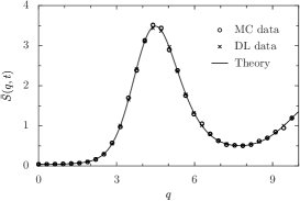
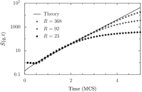
We first consider the critical quench for the antiferromagnet for which we expect stage two kinetics immediately following the quench (refer to Table 1). For this case $M=\beta_{f}$ from Eq. (40). Figure 5 shows the correspondence between the linear theory prediction Eq. (45), the numerical solutions to the dissipative Langevin equation, Eq. (32), averaged over the noise, and the Monte Carlo simulations averaged over the noise. In Fig. 5 the structure factor is plotted versus $q$ at an early time $t=0.125$ MCS (Langevin time is measured in units of MCS). Because we use a square interaction, we plot

$$\bar{S}(q,t)\equiv[S(\pm q,0;t)+S(0,\pm q;t)]/4$$ (48)

instead of taking a circular average. For all simulations presented, we hold the ratio of the system size to the interaction range constant at $L/R\simeq 2.78$ so that the stripe state of the final phase is approximately commensurate with the system size finite .

The coarse-graining employed in the Langevin equation allows us to consider system sizes and interaction ranges which are much larger than those of the Monte Carlo simulations. In Fig. 5 the Monte Carlo simulations have $R=128$, and the Langevin solutions have $R=10^{6}$. The theory curve corresponds to an infinite interaction range (so that the linear theory lasts forever.) Figure 5 shows that the linear theory is still a good approximation at time $t=0.125$ for the Langevin and the Monte Carlo dynamics.

Figure 5: Structure factor $\bar{S}(q,t)\equiv[S(\pm q,0;t)+S(0,\pm q;t)]/4$ versus $q$ for the antiferromagnetic Ising model for early time $t=0.125$ MCS after a critical quench from $T_{i}=\infty$ tp $T_{f}=4T_{c}/9.$ The Monte Carlo data (MC data) has an interaction range of $R=128$, while the numerical solutions to the dissipative Langevin Eq. (32) (DL data) has a range of $10^{6}$. The theory line is a plot of Eq. (45).

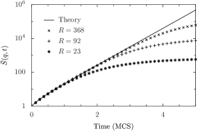
Next we compare the time dependence of $S(\boldsymbol{q},t)$ given by Eq. (45) following a critical quench to our Monte Carlo simulations. Figure 6 shows $\bar{S}(q,t)$ for $q\simeq q^{*}$ plotted against time for several values of $R$ along with the theoretical prediction of Eq. (45). As predicted by Binder (Binder, 1984), we find that stage two kinetics holds for longer times as we increase the interaction range for this value of $q$.

Figure 6: Semi-log plot of the structure factor $\bar{S}(q,t)$ for $q=4.516\simeq q^{*}$ versus time for our Monte Carlo simulations of a critical quench in the antiferromagnetic Ising model. The temperature is quenched from $T_{i}=\infty$ to $T_{f}=4T_{c}/9$. The theory line is a plot of Eq. (45). The duration of the exponential growth increases as the interaction range increases.

V.2.2 Off-critical quenches

For external field quenches or off-critical temperature quenches we find that the short time behavior is independent of $R$, and corresponds to our prediction of stage one kinetics. In Fig. 7 we present the results of off-critical quenches ($T_{i}=\infty$, $h_{i}=0$, $T_{f}=4T_{c}/9$, $h_{f}=0.5$) for $R=23,\>92,\>368$ for Monte Carlo simulations averaged over at least 700 independent initial configurations for each value of $R$. We plot $\bar{S}(q,t)$ versus time for $q=4.516\simeq q^{*}$. We interpret the first Monte Carlo step to be stage one kinetics, which, as we see from Fig. 7 has a time scale that is independent of the interaction range. At about one Monte Carlo step stage two kinetics take over, and the structure factor at $q\simeq q^{*}$ grows exponentially until stage two kinetics breaks down. The break down occurs later for longer interaction ranges. These observations are consistent with the prediction that the time scale of stage one kinetics is determined by the noiseless dynamics of Eq. (22) which is independent of $R$. Note that stage one kinetics were not predicted by the CHC theory.

Figure 7: Semi-log plot of the structure factor $\bar{S}(q,t)$ for $q=4.516\simeq q^{*}$ versus time for Monte Carlo simulations of an off-critical quench in the antiferromagnetic Ising model. The simulation parameters are $T_{i}=\infty$, $T_{f}=\frac{4}{9}T_{c}$, $h_{i}=0$, and $h_{f}=0.5$. The first Monte Carlo step is stage one kinetics, whose time scale is independent of interaction range. The duration of stage two kinetics, marked by exponential evolution, increases as the interaction range increases. The theory line is a plot of Eq. (45) (with $S_{0}(q)$ fit to data) and is only expected to be applicable for stage two.

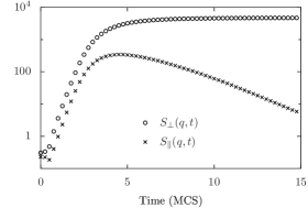
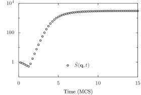
To show that our generalized theory predicts the same behavior for both the disorder to stripes and the disorder to clumps transitions, we compare $S_{\perp}(q,t)$ ($\boldsymbol{q}$ in the direction perpendicular to the final stripe phase) and $S_{\parallel}(q,t)$ ($\boldsymbol{q}$ in the direction parallel to the final stripe phase) where $S_{\perp}(q,t)=S(q^{*},0;t)$ and $S_{\parallel}(q,t)=S(0,q^{*};t)$ for vertical stripes and $S_{\perp}(q,t)=S(0,q^{*};t)$ and $S_{\parallel}=S(q^{*},0;t)$ for horizontal stripes. We find that $S_{\perp}(q,t)$ and $S_{\parallel}(q,t)$ both grow exponentially with the same rate during stage two (see Fig 8(a)). It is not until after stage two that $S_{\parallel}(q,t)$ begins to decrease toward its final value. For comparison, $\bar{S}(q,t)$ is plotted in Fig. 8(b) for the disorder to clumps case. Note that the qualitative behavior for the disorder to stripe and the disorder to clump transitions are the same.

(a)

(b)

Figure 8: (a.)A semi-log plot of $S_{\perp}(q,t)$ (where $\boldsymbol{q}$ is in the direction perpendicular to the final stripe phase) and $S_{\parallel}(q,t)$ (where $\boldsymbol{q}$ is in the direction parallel to the final stripe phase) versus time for an off-critical quench from disorder to stripes with $T_{f}=0.07,$ $h_{f}=0.4$ and $R=92.$ Stage two lasts until about 1.5 MCS, after which $S_{\perp}(q,t)$ and $S_{\parallel}(q,t)$ begin to separate and eventually $S_{\parallel}(q,t)$ decreases towards its stable value. (b.) A semi-log plot of $\bar{S}(q,t)$ for an off-critical quench from disorder to clumps with $T_{f}=0.02,$ $h_{f}=0.8$ and $R=92$ is plotted for comparison.

VI stripes to clumps transition

We now consider the unstable kinetics for spatial symmetry breaking order-to-order transitions. In this section we develop a theory that describes the early time kinetics from an initial stripe state to the stable clump phase following an instantaneous quench of the external field. The development of the theory is analogous to that of the disorder-to-order case, but the periodic structure of the initial configuration of the system introduces some interesting deviations from the CHC theory.

VI.1 Theory

After an external field quench with the temperature held constant, the stable solution to the Euler-Lagrange equation is a clump configuration corresponding to $T_{f}$ and $h_{f}$ (see Fig. 3). We find from numerical solutions to Eq. (32) that there is a second, unstable stripe solution as well, $\phi_{s}(\boldsymbol{r})=\phi_{s}(r_{x})$ where $r_{x}$ and $r_{y}$ represent scaled spatial coordinates (we assume here that the stripes are in the vertical direction).

As in Sec. V, we proceed by considering dissipative dynamics (Eq. (36)) where we choose the mobility to obey Eq. (40), where we now choose $\phi_{0}(\boldsymbol{r})=\phi_{s}(r_{x})$ so that $M(\boldsymbol{r})=M(r_{x})$. Again, the dissipative dynamics and the Glauber dynamics should be equivalent for stage two.

The nonlinear dynamics of Eq. (22) evolves the initial stripe configuration ($\phi_{b}(r_{x},r_{y};t=0)=\phi_{b}(r_{x};t=0)$) toward $\phi_{s}(r_{x}).$ When $\phi_{b}(r_{x},t)\simeq\phi_{s}(r_{x})$, stage two kinetics begins. In this case stage two kinetics is given by Eq. (35) where the mobility $M(r_{x})$ is given by Eq. (40) with $\phi_{0}(\boldsymbol{r})=\phi_{s}(r_{x})$ and $J=-1.$ We find that in order to determine the time dependence of the structure factor for stage two it is sufficient to consider the dynamical equation (35) without the noise term:

$$\frac{\partial\psi(\boldsymbol{r},t)}{\partial t}=-M(r_{x})(\Lambda*\psi)(\boldsymbol{r},t)-\psi(\boldsymbol{r},t).$$ (49)

To understand the behavior of the Fourier modes we Fourier transform Eq. (49):

$$\frac{\partial\psi(q_{x},q_{y};t)}{\partial t} = -\!\int dq_{x}^{\prime}M(q_{x}^{\prime}-q_{x})\Lambda(q_{x}^{\prime},q_{y})\psi(q_{x}^{\prime},q_{y};t)$$ (50)

$$-\psi(q_{x},q_{y};t).$$

Note that in Eq. (50) the $q_{y}$ modes (along the direction of the stripes) are decoupled, but the $q_{x}$ modes (perpendicular to the direction of the stripes) are not. Hence the Fourier modes do not have purely exponential growth as in the disorder-to-order case.

To solve Eq. (50) numerically, we discretize space. For a lattice with $L\times L$ coarse-grained bins, and therefore $L\times L$ Fourier modes, we write $\psi(q_{x},q_{y})$ as $\psi_{ij}$, where $q_{x}$ and $q_{y}$ are $q_{x}=2\pi i/L$ and $q_{y}=2\pi j/L$ for $0\leq i,j<L$. Because the $q_{y}$ variables are decoupled, we choose a particular value $j=j_{0}$ for the remainder of the calculation. The discretized Eq. (50) can be written in matrix form

$$\frac{\partial\psi_{i}(t)}{\partial t}=A_{ik}\psi_{k}(t),$$ (51)

where we have left off the $j=j_{0}$ index. The matrix $A$ is real and has elements

$$A_{ik}=-M_{ik}\Lambda_{k}-\delta_{ik}.$$ (52)

To solve the homogeneous set of equations, $\partial\psi_{i}(t)/\partial t=A_{ik}\psi_{k}(t),$ we diagonalize $A$ to find eigenvectors $v^{\alpha}$ which satisfy:

$$A_{ik}v_{k}^{\alpha}=\lambda^{\alpha}v_{i}^{\alpha},$$ (53)

where the index $\alpha=1,\,2,\,...\,,\,L.$ If the eigenvalues $\lambda^{\alpha}$ are real and distinct (which we have found to be true for the matrices we have numerically diagonalized) then $v^{\alpha}$ form a new basis. We expand $\psi$ in this basis

$$\psi_{i}(t)=\sum_{\alpha}a^{\alpha}(t)v_{i}^{\alpha}.$$ (54)

Equation (51) becomes

$$\frac{\partial}{\partial t}\sum_{\alpha}a^{\alpha}(t)v_{i}^{\alpha}=\sum_{\alpha}a^{\alpha}(t)\lambda^{\alpha}v_{i}^{\alpha}.$$ (55)

Because $v^{\alpha}$ are linearly independent, Eq. (55) can be written as a set of equations:

$$\frac{\partial}{\partial t}a^{\alpha}(t)=a^{\alpha}(t)\lambda^{\alpha},$$ (56)

with solutions

$$a^{\alpha}(t)=a^{\alpha}(0)\textnormal{e}^{\lambda^{\alpha}t}.$$ (57)

The structure factor $S(q_{x}=2\pi i/L,q_{y}=2\pi j_{0}/L;t)=S_{ij_{0}}(t)=\left\langle|\phi_{ij_{0}}(t)|^{2}\right\rangle/V$ due to the noiseless dynamics is

$$S_{ij_{0}}(t) =\frac{\phi_{s,i}^{2}(\delta_{0,i})^{2}}{V}$$

$$\quad+\sum_{\alpha,\alpha^{\prime}}\frac{\left\langle a^{\alpha}(0)a^{\alpha^{\prime}}(0)\right\rangle}{V}e^{(\lambda^{\alpha}+\lambda^{\alpha^{\prime}})t}v_{ij_{0}}^{\alpha}v_{ij_{0}}^{\alpha^{\prime}},$$ (58)

where $\phi_{s,i}=\phi_{s}(q_{x}=2\pi i/L)$ and we expect that $\left\langle a^{\alpha}(0)a^{\alpha^{\prime}}(0)\right\rangle\sim V.$ In the unstable regime, there is at least one positive $\lambda^{\alpha}$ indicating exponential growth. From Eq. (58) we see the exponential growth lasts throughout stage two, but it is growth of eigenvectors that will, in general, mix Fourier modes. We expect, however, that after some time the term in the sum in Eq. (58) which corresponds to the largest positive eigenvalue will dominate, and the growth of Fourier modes will be well approximated by pure exponential growth. Note that we only expect to see exponential growth for near-mean-field systems whose long interaction ranges extend the lifetime of the stage two kinetics to $\tau\sim\ln R$ at the fastest growing eigenvector.

VI.2 Simulation results

VI.2.1 External field quench

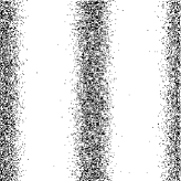
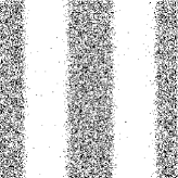
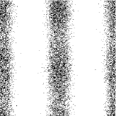
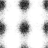
We present the results of Monte Carlo simulations for a quench from a stable stripe configuration with $h_{i}=0$ to $h_{f}=0.8$ at $T_{i}=T_{f}=0.04$. Snapshots following this quench are shown in Fig. 9 for a system with $L=1024$ and interaction range $R=368$. We find that the stripes quickly become less dense and then narrower. Finally, around 10 MCS, the stripes begin to form clumps, and the modulation along the length of the clumps becomes visually perceptible.

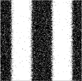t=0.125	t=5.00
t=1.00	t=10.0
t=2.50	t=15.0

Figure 9: Several snapshots showing the initial evolution from an unstable stripe configuration to a clump configuration in the antiferromagnetic Ising model. The lattice size is 1024, the interaction range is 368, and $T_{i}=T_{f}=0.04$. Time is measured in Monte Carlo steps beginning after the external field quench from $h_{i}=0$ to $h_{f}=0.8$. The corresponding structure factor is shown in Fig. 10.

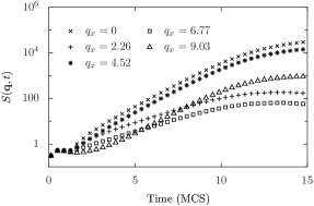
In Fig. 10 we show $S(\boldsymbol{q},t)$ at various values of $\boldsymbol{q}$. We find that the growth is most rapid along the line of modes for which $q_{y}=0$ and the line of modes which is closest to $q_{y}\simeq q^{*}$ (the peak of the Fourier transform of the interaction potential.) In Fig. 10 the Monte Carlo data is averaged over at least 700 initial stripe configurations for the same parameters as the system shown in Fig. 9. We look at several $q_{x}$ modes with $q_{y}\simeq q^{*}$. There is a steep initial increase of $S(q_{x},q_{y})$ and then a gradual decrease during the first Monte Carlo step, which we interpret as stage one kinetics toward the unstable state stripe solution. Stage one corresponds to the initial behavior of the stripes seen in Fig. 9 followed by narrowing of the stripes. Eventually the structure factor modes grow exponentially before stage two kinetics breaks down at around 10 MCS. Two distinct exponential rates are evident.

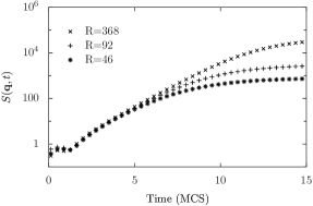
In Fig. 11 we compare the evolution of the structure factor for systems with different interaction ranges. We see that the time scale of stage one kinetics is independent of the interaction range, and exponential behavior lasts longer for larger $R$, as in the CHC theory.

Figure 10: Semi-log plot of the structure factor $S(\boldsymbol{q},t)$ versus time in the antiferromagnetic Ising model with $R=368$ for various values of $q_{x}$ for $q_{y}\simeq q^{*}$ following a quench from $h_{i}=0$ to $h_{f}=0.8$ at $T_{i}=T_{f}=0.04$. The Monte Carlo data is averaged over about 700 independent stripe configurations. We interpret the first Monte Carlo step to be stage one kinetics. After this time stage two takes over. At the beginning of stage two, the Fourier modes do not grow exponentially. Eventually they grow exponentially at two different rates (starting from about 4 Monte Carlo steps). This exponential growth lasts until about 10 Monte Carlo steps for $R=368$.

Figure 11: Semi-log plot of the structure factor $S(\boldsymbol{q},t)$ at $q_{x}=0$ and $q_{y}\simeq q^{*}$ versus time in the antiferromagnetic Ising model for interaction ranges $R=46,\>92$, and $368$. The quench parameters are the same as those in Fig. 10. We find that the time scale of stage one kinetics (about the first MCS) is independent of $R$, and the exponential evolution of stage two lasts longer for longer $R$.

VI.2.2 Understanding stage two kinetics

To better understand the behavior of the system during stage two, we seek an analogy to the critical quench where stage one is entirely absent from the early unstable evolution. Thus, instead of quenching the field, we will initially prepare our system in the state corresponding to the unstable Euler-Lagrange solution.

We verify numerically that the unstable stripe solution $\phi_{s}(r_{x},r_{y})$ to the Euler-Lagrange equation at a particular $T$ and $h$ corresponds to the $one-dimensional$ stable clump solution $\phi_{\rm 1D}(r_{x})$ with the same temperature and external field: $\phi_{s}(r_{x},r_{y})=\phi_{s}(r_{x})=\phi_{\rm 1D}(r_{x})$.

For the stripe to clump transition we used the $h_{f}=0.8$ and $T_{f}=0.04$. We find the stable one-dimensional solution by numerically solving Eq. (32) in one dimension at this field and temperature. We use the corresponding unstable stripe solution $\phi_{s}(r_{x})$ to find the matrix $A$ in Eq. (52) which depends on $\phi_{s}(r_{x})$ through the mobility $M(r_{x})=\beta_{f}(1-\phi_{s}(r_{x})^{2})$.

For the parameters considered ($h_{f}=0.8$, $T_{f}=0.04$, $L=1024$, and $L/R\simeq 2.78$), we diagonalize $A$ and find two positive eigenvalues of Eq. (53) (Larger lattice sizes give a larger number of positive eigenvalues. The depth of the quench also effects the number of positive eigenvalues.) We also find by examining the eigenvectors corresponding to these two positive eigenvalues that each Fourier mode has a non-zero contribution from only one of the two positive eigenvalues. Thus we expect each Fourier mode to be dominated by one of the two exponential terms with a positive argument and two distinct exponential growth rates should eventually be apparent. This is consistent with the data shown in Figs. 12 and 13.

Figure 12: Semi-log plot of the structure factor versus time in the antiferromagnetic Ising model for various $q_{x}$ values with $q_{y}=4.518$. The initial configuration is constructed from the one-dimensional solution $\phi_{\rm 1D}$ to the Euler-Lagrange equation at temperature $T=0.04$ and field $h=0.8$. Data is averaged over about 700 independent stripe configurations. Two distinct exponential growth rates are apparent from about 3 to 8 Monte Carlo steps.

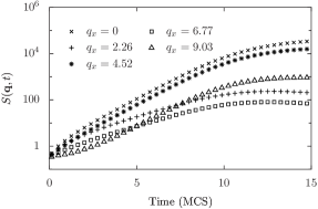
The one-dimensional solution is used to construct initial two-dimensional configurations for the Monte Carlo simulations. The length of the one-dimensional coarse grained lattice is chosen to be the same as the length of the two-dimensional Monte Carlo lattice. We use the value of $\phi_{s}(r_{x})$ to determine the probability that the corresponding Ising spin is initially up: $p=(\phi_{s}(r_{x})+1)/2$. We repeat this process over all horizontal strips of the Ising lattice. We then run the Monte Carlo simulation and monitor $S(\boldsymbol{q},t)$ for various values of $\boldsymbol{q}$, averaging over independent runs. As expected, the evolution looks similar to the evolution of the corresponding $S(\boldsymbol{q},t)$ in Fig. 10 with about the first Monte Carlo step removed. In Fig. 13 we have plotted two Fourier modes from Fig. 12 along with the exponential curves from Eq. (58) to indicate the growth rates predicted from our matrix calculation.

Figure 13: A semi-log plot of structure factor for two Fourier modes from Fig. 12 along with predictions for linear theory exponential growth, $f_{1}(t)\sim\exp(2\lambda_{1}t)$ and $f_{2}(t)\sim\exp(2\lambda_{2}t)$, where the $S$ intercept has been fit to the data. Here $\lambda_{1}$ and $\lambda_{2}$ are the two positive eigenvalues from our matrix calculation.

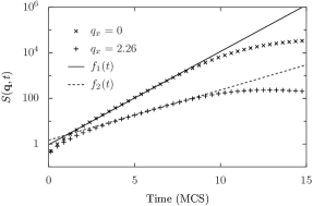
After some initial evolution the Fourier modes eventually grow exponentially at one of two rates, reflecting the coupling of the modes due to the spatial variation of the initial state.

The fact that our theory predicts exponential growth rates even though we did not consider the effect of the noise on the structure factor indicates that, as in the disorder-to-order case, the contribution from the noise term has the same time dependence as the noiseless part, at least at later times during stage two noise .

VII summary and discussion

We have presented a generalization of the linear theory of Cahn, Hilliard, and Cook (Cahn and Hilliard, 1958, 1959; Cahn1967, ; Cook1970, ) for early stage unstable evolution. In particular, we have given a description of the initial unstable evolution for transitions with spatial symmetry breaking and no order parameter conservation. One of our predictions is that there are two stages of early time kinetics in general for systems with long interaction ranges. Stage one is dominated by a symmetry preserving nonlinear dynamics and takes the system to a symmetry constrained local minimum of the free energy on a time scale that is independent of the interaction range. Although noise driven fluctuations may also be growing during stage one, they do not evolve significantly in this relatively short-lived regime. In stage two these noise driven fluctuations break the spatial symmetry of the initial configuration and grow for an extended period of time.

This picture is consistent with the observed behavior of the long-range antiferromagnetic Ising model, a system that exhibits several symmetry breaking transitions. We find the stage two kinetics of the long-range antiferromagnetic Ising model is characterized by long-lived exponential growth of symmetry breaking fluctuations. For the disorder-to-order case the symmetry breaking fluctuations are individual Fourier modes. In contrast, the order-to-order case is complicated by the spatial symmetry of the initial configuration, which couples the growth of the Fourier modes. For this reason the symmetry breaking fluctuations in the order-to-order case are not individual Fourier modes, but eigenvectors in Fourier space. The evolution of the Fourier modes is described by linear combinations of exponential growth and/or decay, which after some time resembles pure exponential growth due to the largest positive eigenvalue.

We have focused on systems without order parameter conservation. A future publication will apply our generalized theory for order-to-order transitions with order parameter conserving dynamics.

Our results have several consequences for experimentalists and simulators looking to fit their data to a linear theory after an unstable quench. For disorder-to-order transitions stage two kinetics, which is analogous to the CHC theory, is expected immediately after the quench only for systems with conserved order parameters or only in special circumstances for systems with no conserved order parameters (as in a critical quench.) For order-to-order transitions, exponential growth of Fourier modes is delayed for two reasons. In stage one exponential growth is not expected. In stage two the evolution of Fourier modes is represented by a linear combination of exponential terms, and therefore only approximate exponential evolution is expected after some time. Because the lifetime of stage two kinetics is limited by the finite interaction range, exponential Fourier mode growth may be absent even if the linear evolution of stage two is present.