Approximate Conditional Distributions of Distances Between Nodes in a Two-Dimensional Sensor Network

Abstract

When we represent a network of sensors in Euclidean space by a graph, there are two distances between any two nodes that we may consider. One of them is the Euclidean distance. The other is the distance between the two nodes in the graph, defined to be the number of edges on a shortest path between them. In this paper, we consider a network of sensors placed uniformly at random in a two-dimensional region and study two conditional distributions related to these distances. The first is the probability distribution of distances in the graph, conditioned on Euclidean distances; the other is the probability density function associated with Euclidean distances, conditioned on distances in the graph. We study these distributions both analytically (when feasible) and by means of simulations. To the best of our knowledge, our results constitute the first of their kind and open up the possibility of discovering improved solutions to certain sensor-network problems, as for example sensor localization.

Keywords: Sensor networks, Random geometric graphs, Distance distributions.

1 Introduction

We consider a network of $n$ sensors, each one placed at a fixed position in two-dimensional space and capable of communicating with another sensor if and only if the Euclidean distance between the two is at most $R$, for some constant radius $R>0$. If $\delta_{ij}$ denotes this distance for sensors $i$ and $j$, then a graph representation of the network can be obtained by letting each sensor be a node and creating an edge between any two distinct nodes $i$ and $j$ such that $\delta_{ij}\leq R$. Such a representation is, aside from a scale factor, equivalent to a unit disk graph [9].

Often $n$ is a very large integer and the network is essentially unstructured, in the sense that the sensors’ positions, although fixed, are generally unknown. In domains for which this holds, generalizing the graph representation in such a way that each node’s position is given by random variables becomes a crucial step, since it opens the way to the investigation of relevant distributions related to all networks that result from the same deployment process. Such a generalization, which can be done for any number of dimensions, is known as a random geometric graph [32]. Similarly to the random graphs of Erdős and Rényi [13] and related structures [29], many important properties of random geometric graphs are known, including some related to connectivity and the appearance of the giant component [1, 2, 3] and others more closely related to applications [26, 18, 24].

One curious aspect of random geometric graphs is that, if nodes are positioned uniformly at random, the expected Euclidean distance between any two nodes is a constant in the limit of very large $n$, depending only on the number of dimensions (two, in our case) [6]. In this case, distance-dependent analyses must necessarily couple the Euclidean distance with some other type of distance between nodes. The natural candidate is the standard graph-theoretic distance between two nodes, given by the number of edges on a shortest path between them [7]. For nodes $i$ and $j$, this distance is henceforth denoted by $d_{ij}$ and referred to simply as the distance between $i$ and $j$.

Given $i$ and $j$, the Euclidean distance $\delta_{ij}$ and the distance $d_{ij}$ between the two nodes are not independent of each other, but rather interrelate in a complex way. Our goal in this paper is to explore the relationship between the two when all sensors are positioned uniformly at random in a given two-dimensional region. Specifically, for $i$ and $j$ two distinct nodes chosen at random, we study the probability that $d_{ij}=d$ for some integer $d>0$, given that $\delta_{ij}=\delta$ for some real number $\delta\geq 0$. Similarly, we also study the probability density associated with $\delta_{ij}=\delta$ when $d_{ij}=d$. Our study is analytical whenever feasible, but is also computational throughout. Depending on the value of $d$, we are in a few cases capable of providing exact closed-form expressions, but in general what we give are approximations, either derived mathematically or inferred from simulation data exclusively.

We remark, before proceeding, that we perceive the study of distance-related distributions for random geometric graphs as having great applicability in the field of sensor networks, particularly in domains in which it is important for each sensor to have a good estimate of its location. In fact, of all possible applications that we normally envisage for sensor networks [15], network localization is crucial in all cases that require the sensed data to be tagged with reliable indications of where the data come from; it has also been shown to be important even for routing purposes [23]. So, although we do not dwell on the issue of network localization anywhere else in the paper, we now digress momentarily to clarify what we think the impact of distance-related distributions may be.

The problem of network localization has been tackled from a variety of perspectives, including rigidity-theoretic studies [14, 4], approaches that are primarily algorithmic, either centralized [12, 34] or distributed [19, 31, 25, 27], and others that generalize on our assumptions by taking advantage of sensor mobility [21, 27] or uneven radii [22]. In general one assumes the existence of some anchor sensors (regularly placed [8] or otherwise), for which positions are known precisely, and then the problem becomes reduced to the problem of providing, for each of the other sensors, the Euclidean distances that separate it from three of the anchors (its tripolar coordinates with respect to those anchors, from which the sensor’s position can be easily calculated [37]).

Finding a sensor’s Euclidean distance to an anchor is not simple, though. Sometimes signal propagation is used for direct or indirect measurement [5, 20, 33, 17, 36, 30], but there are approaches that rely on no such techniques [28, 8, 31]. The latter include one of the most successful distributed approaches [31], which nonetheless suffers from increasing lack of accuracy as sparsity or irregularity in sensor positioning become more pronounced. The algorithm of [31] assumes, for each anchor $i$, that each edge on any shortest path to $i$ is equivalent to a fixed Euclidean distance, which is estimated by $i$ in communication with the other anchors and by simple proportionality can be used by any node to infer its Euclidean distance to $i$. We believe that knowledge of distance-related distributions has an important role to play in replacing this assumption and perhaps dispelling the algorithm’s difficulties in the less favorable circumstances alluded to above.

We proceed in the following manner. In Section 2 we give some notation and establish the overall approach to be followed when pursuing the analytical characterization of distance-related distributions. Then in Sections 3 through 5 we present the mathematical analysis of the $d=1$ through $d=3$ cases. We continue in Section 6 with computational results related to $d\geq 1$ and close in Section 7 with some discussion and concluding remarks.

2 Overall approach

Let $i$ and $j$ be two distinct, randomly chosen nodes. For $d>0$ an integer and $\delta\geq 0$ a real number, we use $P_{\delta}(d)$ to denote the probability, conditioned on $\delta_{ij}=\delta$, that $d_{ij}=d$. Likewise, we use $p_{d}(\delta)$ to denote the probability density, conditioned on $d_{ij}=d$, associated with $\delta_{ij}=\delta$. These two quantities relate to each other in the standard way of combining integer and continuous random variables [35].

If we assume that $P_{\delta}(d)$ is known for all applicable values of $d$ and $\delta$, then it follows from Bayes’ theorem that

$$p_{d}(\delta)=\frac{P_{\delta}(d)p(\delta)}{P(d)},$$ (1)

where $p(\delta)$ is the unconditional probability density associated with the occurrence of an Euclidean distance of $\delta$ separating two randomly chosen nodes and $P(d)$ is the unconditional probability that the distance between them is $d$. Clearly, $P(d)=\int_{r=0}^{dR}P_{r}(d)p(r)\mathrm{d}r$, since $P_{r}(d)=0$ for $r>dR$. Moreover, $p(r)$ is proportional to the circumference of a radius-$r$ circle, $2\pi r$, which yields

$$p_{d}(\delta)=\frac{P_{\delta}(d)\delta}{\int_{r=0}^{dR}P_{r}(d)r\mathrm{d}r}.$$ (2)

In view of Equation (2), our approach henceforth is to concentrate on calculating $P_{\delta}(d)$ for all appropriate values of $d$ and $\delta$, and then to use the equation to obtain $p_{d}(\delta)$. In order to calculate $P_{\delta}(d)$, we fix two nodes $a$ and $b$ such that $\delta_{ab}=\delta$ and proceed by analyzing how the two radius-$R$ circles (the one centered at $a$ and the one at $b$) relate to each other. While doing so, we assume that the two-dimensional region containing the graph has unit area, so that the area of any of its sub-regions automatically gives the probability that it contains a randomly chosen node. We assume further that all border effects can be safely ignored (but see Section 6 for the computational setup that justifies this).

3 The distance-1 and distance-2 cases

The case of $d=1$ is straightforward, since $d_{ab}=d$ if and only if $\delta\leq R$. Consequently,

$$P_{\delta}(1)=\cases{1,&if $\delta\leq R$;\cr 0,&otherwise}$$ (3)

and, by Equation (2),

$$p_{1}(\delta)=\cases{2\delta/R^{2},&if $\delta\leq R$;\cr 0,&otherwise.}$$ (4)

For $d=2$, we have $d_{ab}=d$ if and only if $\delta>R$ and at least one node $k$ exists, with $k\notin\{a,b\}$, such that $\delta_{ak}\leq R$ and $\delta_{bk}\leq R$. The probability that this holds for a randomly chose $k$ is given by the intersection area of the radius-$R$ circles centered at $a$ and $b$, here denoted by $\rho_{\delta}$. From [37], we have

$$\rho_{\delta}=\cases{2R^{2}\cos^{-1}\left(\delta/2R\right)-\delta\sqrt{R^{2}-\delta^{2}/4},&if $\delta\leq 2R$;\cr 0,&otherwise.}$$ (5)

Because any node that is not $a$ or $b$ may, independently, belong to such intersection, we have

$$P_{\delta}(2)=\cases{1-(1-\rho_{\delta})^{n-2},&if $\delta>R$;\cr 0,&otherwise.}$$ (6)

As for $p_{2}(\delta)$, it is as given by Equation (2), equaling $0$ if $\delta\leq R$ or $\delta>2R$ (we remark that a closed-form expression is obtainable also in this case, but it is too cumbersome and is for this reason omitted).

4 The distance-3 case: exact basis

The $d=3$ case is substantially more complex than its predecessors in Section 3. We begin by noting that $d_{ab}=d$ if and only if the following three conditions hold:

• $\delta>R$.

• No node $i$ exists such that both $\delta_{ai}\leq R$ and $\delta_{bi}\leq R$.

• At least one node $k\notin\{a,b\}$ exists, and for this $k$ at least one node $\ell\notin\{a,b,k\}$, such that $\delta_{ak}\leq R$, $\delta_{k\ell}\leq R$, $\delta_{b\ell}\leq R$, $\delta_{a\ell}>R$, and finally $\delta_{bk}>R$.

For each fixed $k$ and $\ell$ in Condition C3, these three conditions result from the requirement that nodes $a$, $k$, $\ell$, and $b$, in this order, constitute a shortest path from $a$ to $b$.

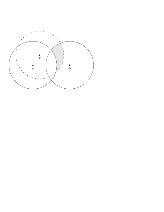
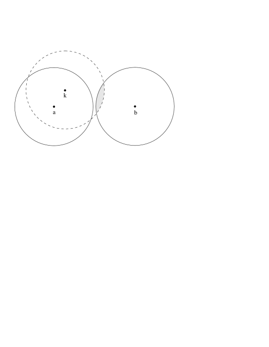
If we fix some node $k\notin\{a,b\}$ for which $\delta_{ak}\leq R$ and $\delta_{bk}>R$, the probability that Condition C3 is satisfied by $k$ and a randomly chosen $\ell$ is a function of intersection areas of circles that varies from case to case, depending on the value of $\delta$. There are two cases to be considered, as illustrated in Figure 1. In the first case, illustrated in part (a) of the figure, $R<\delta\leq 2R$ and node $\ell$ is to be found in the intersection of the radius-$R$ circles centered at $b$ and $k$, provided it is not also in the radius-$R$ circle centered at $a$. The intersection area of interest results from computing the intersection area of two circles (those centered at $b$ and $k$) and subtracting from it the intersection area of three circles (those centered at $a$, $b$, and $k$). The former of these intersection areas is given as in Equation (5), with $\delta_{bk}$ substituting for $\delta$; as for the latter, closed-form expressions also exist, as given in [16]. The second case, shown in part (b) of Figure 1, is that of $2R<\delta\leq 3R$, and then the intersection area of interest is the one of the circles centered at $b$ and $k$. Regardless of which case it is, we use $\sigma_{\delta}^{k}$ to denote the resulting area. Thus, the probability that at least one $\ell$ exists for fixed $k$ is $1-(1-\sigma_{\delta}^{k})^{n-3}$.

(a)

(b)

Figure 1: Regions (shown in shades) whose areas yield the value of $\sigma_{\delta}^{k}$ for $R<\delta\leq 2R$ (a) and $2R<\delta\leq 3R$ (b).

Now let $P^{\prime}_{\delta}(3)$ be the probability that a randomly chosen $k$ satisfies Condition C3. Let also $K_{\delta}$ be the region inside which such a node can be found with nonzero probability. If $x_{k}$ and $y_{k}$ are the Cartesian coordinates of node $k$, then each possible location of $k$ inside $K_{\delta}$ contributes to $P^{\prime}_{\delta}(3)$ the infinitesimal probability $[1-(1-\sigma_{\delta}^{k})^{n-3}]\mathrm{d}x_{k}\mathrm{d}y_{k}$. It follows that

$$P^{\prime}_{\delta}(3)=\int_{k\in K_{\delta}}[1-(1-\sigma_{\delta}^{k})^{n-3}]\mathrm{d}x_{k}\mathrm{d}y_{k}.$$ (7)

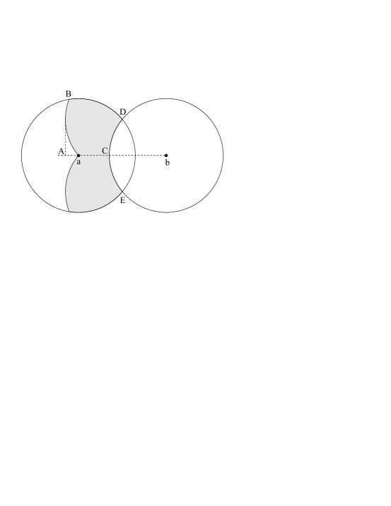
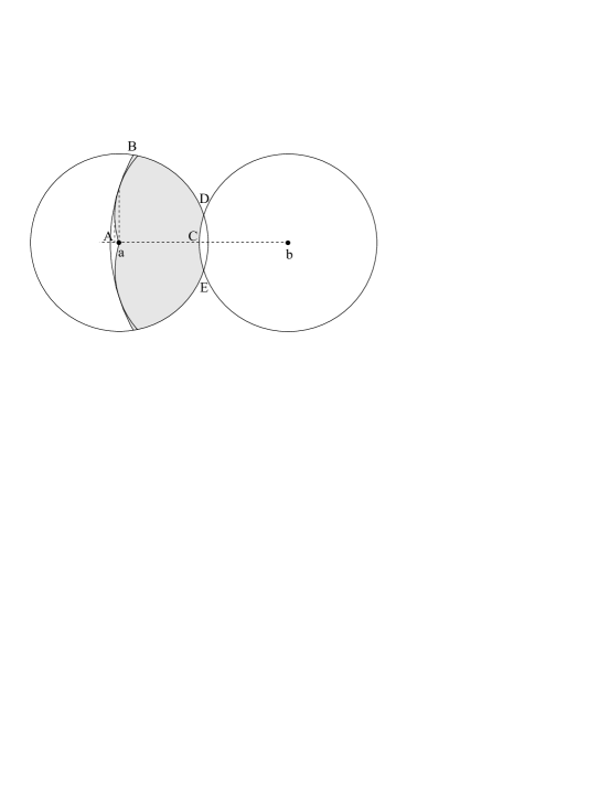
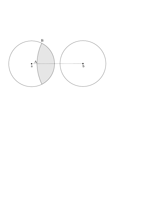
There are three possibilities for the region $K_{\delta}$, shown in parts (a) through (c) of Figure 2 as shaded regions, respectively for $R<\delta\leq R\sqrt{3}$, $R\sqrt{3}<\delta\leq 2R$, and $2R<\delta\leq 3R$. The shaded region in part (a) is delimited by four radius-$R$ circles, the ones centered at nodes $a$ (above and below) and $b$ (on the right) and the ones centered at points $D$ and $E$ (on the left). As $\delta$ gets increased beyond $R\sqrt{3}$—and, at the threshold, point $D$ becomes collinear with point $B$ and node $b$—we move into part (b) of the figure, where the shaded region is now delimited on the left either by the radius-$R$ circles centered at $D$ and $E$ or by the radius-$2R$ circle centered at $b$, depending on the point of common tangent between each of the radius-$R$ circles and the radius-$2R$ circle. The next threshold leads $\delta$ beyond $2R$, and in part (c) of the figure the shaded region is delimited on the left by the radius-$2R$ circle centered at $b$, on the right by the radius-$R$ circle centered at $a$.

(a)

(b)

(c)

Figure 2: Regions (shown in shades) where node $k$ can be found with nonzero probability for $R<\delta\leq R\sqrt{3}$ (a), $R\sqrt{3}<\delta\leq 2R$ (b), and $2R<\delta\leq 3R$ (c).

Figure 2 is also useful in helping us obtain a more operational version of the expression for $P^{\prime}_{\delta}(3)$, to be used in Section 6. First we establish a Cartesian coordinate system by placing its origin at node $a$ and making the positive abscissa axis go through node $b$. In this system, the shaded regions in all of parts (a) through (c) of the figure are symmetrical with respect to the abscissa axis. If for each value of $x_{k}$ we let $y_{k}^{-}(x_{k})$ and $y_{k}^{+}(x_{k})$ be, respectively, the minimum and maximum $y_{k}$ values in the upper half of the shaded region for the value of $\delta$ at hand, then

$$P^{\prime}_{\delta}(3)=2\int_{x_{k}=x_{k}^{-}}^{x_{k}^{+}}\int_{y_{k}=y_{k}^{-}(x_{k})}^{y_{k}^{+}(x_{k})}[1-(1-\sigma_{\delta}^{k})^{n-3}]\mathrm{d}x_{k}\mathrm{d}y_{k},$$ (8)

where $x_{k}^{-}$ and $x_{k}^{+}$ bound the possible values of $x_{k}$ for the given $\delta$.

All pertinent values of $x_{k}^{-}$ and $x_{k}^{+}$, as well as of $y_{k}^{-}(x_{k})$ and $y_{k}^{+}(x_{k})$, are given in Table 1, where $\delta^{-}$ and $\delta^{+}$ indicate, respectively, the lower and upper limit for $\delta$ in each of the three possible cases. This table’s entries make reference to the abscissae of points $A$, $B$, $C$, and $D$ (respectively $x_{A}$, $x_{B}$, $x_{C}$, and $x_{D}$) and to the ordinate of point $D$ ($y_{D}$). These are given in Table 2.

Table 1: Cartesian coordinates delimiting the upper halves of shaded regions in Figure 2.

$\delta^{-}$	$\delta^{+}$	$x_{k}^{-}$	$x_{k}^{+}$	$y_{k}^{-}(x_{k})$	$y_{k}^{+}(x_{k})$	Fig.
$R$	$R\sqrt{3}$	$x_{A}$	$x_{B}$	$y_{D}-\sqrt{R^{2}-(x_{k}-x_{D})^{2}}$	$y_{D}+\sqrt{R^{2}-(x_{k}-x_{D})^{2}}$	2(a)
		$x_{B}$	$0$	$y_{D}-\sqrt{R^{2}-(x_{k}-x_{D})^{2}}$	$\sqrt{R^{2}-x_{k}^{2}}$
		$0$	$x_{C}$	$0$	$\sqrt{R^{2}-x_{k}^{2}}$
		$x_{C}$	$x_{D}$	$\sqrt{R^{2}-(x_{k}-\delta)^{2}}$	$\sqrt{R^{2}-x_{k}^{2}}$
$R\sqrt{3}$	$2R$	$x_{A}$	$0$	$y_{D}-\sqrt{R^{2}-(x_{k}-x_{D})^{2}}$	$y_{D}+\sqrt{R^{2}-(x_{k}-x_{D})^{2}}$	2(b)
		$0$	$x_{B}$	$0$	$\sqrt{4R^{2}-(x_{k}-\delta)^{2}}$
		$x_{B}$	$x_{C}$	$0$	$\sqrt{R^{2}-x_{k}^{2}}$
		$x_{C}$	$x_{D}$	$\sqrt{R^{2}-(x_{k}-\delta)^{2}}$	$\sqrt{R^{2}-x_{k}^{2}}$
$2R$	$3R$	$x_{A}$	$x_{B}$	$0$	$\sqrt{4R^{2}-(x_{k}-\delta)^{2}}$	2(c)
		$x_{B}$	$R$	$0$	$\sqrt{R^{2}-x_{k}^{2}}$

Table 2: Cartesian coordinates used in Table 1.

$\delta^{-}$	$\delta^{+}$	$x_{A}$	$x_{B}$	$x_{C}$	$x_{D}$	$y_{D}$	Fig.
$R$	$R\sqrt{3}$	$\delta/2-R$	$\left(\delta-\sqrt{3(4R^{2}-\delta^{2})}\,\right)/4$	$\delta-R$	$\delta/2$	$\sqrt{4R^{2}-\delta^{2}}/2$	2(a)
$R\sqrt{3}$	$2R$	$\delta/2-R$	$(\delta^{2}-3R^{2})/2\delta$	$\delta-R$	$\delta/2$	$\sqrt{4R^{2}-\delta^{2}}/2$	2(b)
$2R$	$3R$	$\delta-2R$	$(\delta^{2}-3R^{2})/2\delta$				2(c)

5 The distance-3 case: approximate extension

Obtaining $P_{\delta}(3)$ from $P^{\prime}_{\delta}(3)$ requires that we fulfill the remaining requirements set by Conditions C2 and C3 in Section 4. These are that no node exists in the intersection of the radius-$R$ circles centered at $a$ and $b$ and that at least one node $k$ exists with the properties given in Condition C3. While the probability of the former requirement is simply $(1-\rho_{\delta})^{n-2}$, expressing the probability of the latter demands that we make a careful approximation to compensate for the lack of independence of certain events with respect to one another.

For node $i\notin\{a,b\}$, let $\epsilon_{i}$ stand for the event that Condition C3 does not hold for $k=i$. Let also $Q_{\delta}(\epsilon_{i})$ be the probability of $\epsilon_{i}$ and $Q_{\delta}$ the joint probability of all $n-2$ events. Clearly, $Q_{\delta}(\epsilon_{i})=1-P^{\prime}_{\delta}(3)$ for any $i$ and, for $\delta>R$, $P_{\delta}(3)=(1-Q_{\delta})(1-\rho_{\delta})^{n-2}$. Therefore, if all the $n-2$ events were independent of one another, we would have

$$Q_{\delta}=\prod_{i\notin\{a,b\}}Q_{\delta}(\epsilon_{i})=[1-P^{\prime}_{\delta}(3)]^{n-2}$$ (9)

and, consequently,

$$P_{\delta}(3)=\cases{\{1-[1-P^{\prime}_{\delta}(3)]^{n-2}\}(1-\rho_{\delta})^{n-2},&if $\delta>R$;\cr 0,&otherwise.}$$ (10)

However, once we know of a certain node $i$ that Condition C3 does not hold for it, immediately we reassess as less likely that the condition holds for nodes in the Euclidean vicinity of $i$. The $n-2$ events introduced above are then not unconditionally independent of one another, although we do expect whatever degree of dependence there is to wane progressively as we move away from node $i$.

We build on this intuition by postulating the existence of an integer $n^{\prime}<n-2$ such that the independence of the $n^{\prime}$ events not only holds but is also sufficient to determine $P_{\delta}(3)$ as indicated above, provided the corresponding $n^{\prime}$ nodes are picked uniformly at random. But since this is precisely the way in which, by assumption, sensors are positioned, it suffices that any $n^{\prime}$ nodes be selected, yielding

$$P_{\delta}(3)=\cases{\{1-[1-P^{\prime}_{\delta}(3)]^{n^{\prime}}\}(1-\rho_{\delta})^{n-2},&if $\delta>R$;\cr 0,&otherwise.}$$ (11)

Similarly to the previous cases, $p_{3}(\delta)$ is given by Equation (2) and equals $0$ if $\delta\leq R$ or $\delta>3R$.

It remains, of course, for the value of $n^{\prime}$ to be discovered if our postulate is to be validated. We have done this empirically, by means of computer simulations, as discussed in Section 6.

6 Computational results

In this section we present simulation results and, for $d=1,2,3$, contrast them with the analytic predictions of Sections 3 through 5. The latter are obtained by numerical integration when a closed-form expression is not available (the case of $d=3$ also requires simulations for finding $n^{\prime}$; see below). For $d>3$, we demonstrate that good approximations by Gaussians can be obtained.

We use $n=1\,000$ and a circular region of unit area, therefore of radius $\sqrt{1/\pi}\approx 0.564$, for the placement of nodes. Node $a$ is always placed at the circle’s center, which has Cartesian coordinates $(0,0)$, and all results refer to distances to $a$. Our choice for the value of $R$ depends on the expected number of neighbors (or connectivity) of a node, which we denote by $z$ and use as the main parameter. Since $z=\pi R^{2}n$ for large $n$, choosing the value of $z$ immediately yields the value of $R$ to be used. We use $z=3\pi$ and $z=5\pi$, which yield, respectively, $R\approx 0.055$ and $R\approx 0.071$. We note that both values of $z$ are significantly above the phase transition that gives rise to the giant component, which happens at $z\approx 4.52$ [11]. In all our experiments, then, graphs are connected with high probability.

For each value of $z$, each simulation result we present is an average over $10^{6}$ independent trials. Each trial uses a matrix of accumulators having $n-1$ rows (one for each of the possible distance values) and $1\,000\sqrt{1/\pi}$ columns (one for each of the $0.001$-wide bins into which Euclidean distances are compartmentalized). A trial consists of: placing $n-1$ nodes uniformly at random in the circle; computing the Euclidean distance between each node and node $a$; computing the distances between each node and node $a$ (this is done with Dijkstra’s algorithm [10]); updating the accumulator that corresponds to each node, given its two distances. At the end of each trial, its contributions to $P_{\delta}(d)$ and $p_{d}(\delta)$ are computed, with $d=1,2,\ldots,n-1$ and $\delta$ ranging through the middle points of all bins. If $M$ is the matrix of accumulators, then these contributions are given, respectively, by $M(d,\delta)/\sum_{d^{\prime}}M(d^{\prime},\delta)$ and $M(d,\delta)/0.001\sum_{\delta^{\prime}}M(d,\delta^{\prime})$.

The case of $d=3$ requires two additional simulation procedures, one for determining simulation data for $P^{\prime}_{\delta}(3)$, the other to determine $n^{\prime}$ for use in obtaining analytic predictions for $P_{\delta}(3)$. The former of these fixes node $b$ at coordinates $(\delta,0)$ and performs $10^{7}$ independent trials. At each trial, two nodes are generated uniformly at random in the circle. At the end of all trials, the desired probability is computed as the fraction of trials that resulted in nodes $k$ and $\ell$ as in Section 4.

The simulation for the determination of $n^{\prime}$ is conducted for $\delta=2R$ only, whence $\rho_{\delta}=0$. This is the value of $\delta$ for which the results from the simulation above for $P_{\delta}(3)$ and the analytic prediction for $1-[1-P^{\prime}_{\delta}(3)]^{n-2}$ differ the most (data not shown). Moreover, as we will see shortly, the value of $n^{\prime}$ we find using this value of $\delta$ is good for all other values as well. The simulation is aimed at finding the value of $Q_{\delta}$ and proceeds in $10^{9}$ independent trials. Each trial fixes node $b$ at $(\delta,0)$ and places the remaining $n-2$ nodes in the circle uniformly at random. The fraction of trials resulting in no node qualifying as the node $k$ of Section 4 is the value of $Q_{\delta}$. We set $n^{\prime}$ to be the $m<n-2$ that minimizes $|Q_{\delta}-[1-P^{\prime}_{\delta}(3)]^{m}|$, where $P^{\prime}_{\delta}(3)$ refers to the analytic prediction. Our results are $n^{\prime}=779$ for $z=3\pi$, $n^{\prime}=780$ for $z=5\pi$.

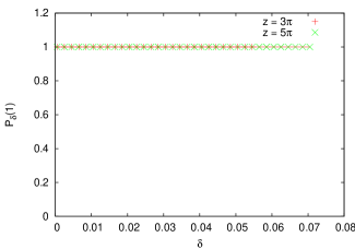
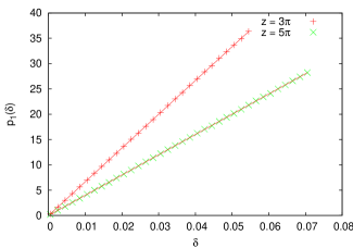
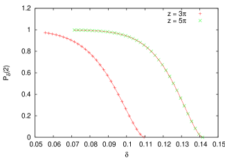
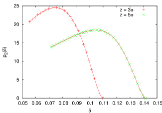
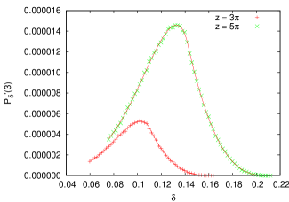
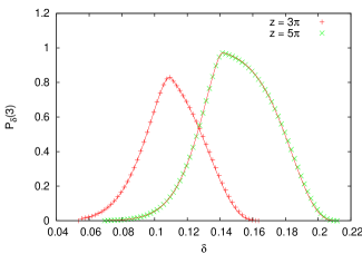
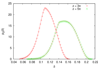
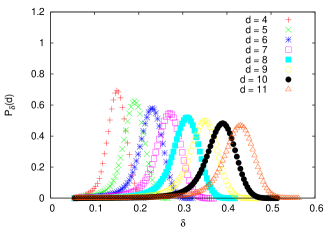
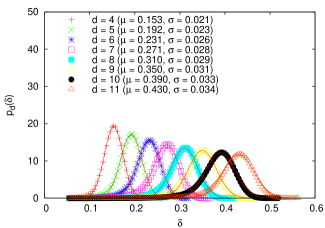
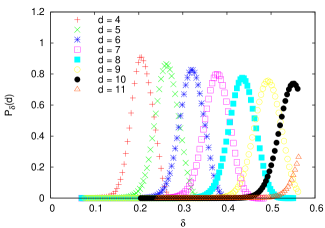
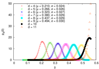
Results for $d=1$ are shown in Figure 3, for $d=2$ in Figure 4, for $d=3$ in Figures 5 and 6, and for $d>3$ in Figure 7. In all figures, both $P_{\delta}(d)$ and $p_{d}(\delta)$ are plotted against $\delta$, since it seems better to visualize what happens as one gets progressively farther from node $a$ in Euclidean terms. For this reason, the plots for $P_{\delta}(d)$ do not constitute a probability distribution for any fixed value of $d$.

(a)

(b)

Figure 3: $P_{\delta}(1)$ (a) and $p_{1}(\delta)$ (b). Solid lines give the analytic predictions.

(a)

(b)

Figure 4: $P_{\delta}(2)$ (a) and $p_{2}(\delta)$ (b). Solid lines give the analytic predictions.

Figure 5: $P^{\prime}_{\delta}(3)$. Solid lines give the analytic predictions.

(a)

(b)

Figure 6: $P_{\delta}(3)$ (a) and $p_{3}(\delta)$ (b). Solid lines give the analytic predictions.

(a)

(b)

Figure 7: $P_{\delta}(d)$ and $p_{d}(\delta)$ for $d>3$, with $z=3\pi$ (a, b) and $z=5\pi$ (c, d). Solid lines give the Gaussians that best fit some of the $p_{d}(\delta)$ data, each of mean $\mu$ and standard deviation $\sigma$ as indicated.

(c)

(d)

Figure 7: Continued.

7 Discussion and conclusion

The results summarized in Figures 3 through 6 reveal excellent agreement between the analytic predictions we derived in Sections 3 through 5 and our simulation data. This holds not only for the simple cases of $d=1$ and $d=2$, but also for the considerably more complex cases of $P^{\prime}_{\delta}(3)$ and $P_{\delta}(3)$. The latter, in particular, depends on the empirically determined $n^{\prime}$. In this respect, it is clear from Figure 6 that, even though $n^{\prime}$ could have been calculated for a greater assortment of $\delta$ values, doing it exclusively for $\delta=2R$ seems to have been sufficient.

Figure 7 contemplates some of the $d>3$ cases, for which we derived no analytic predictions. The values of $d$ that the figure covers in parts (a, b) and (c, d), respectively for $z=3\pi$ and $z=5\pi$, are $4,\ldots,11$. Of these, $d=11$ for $z=5\pi$ in part (d) typifies what happens for larger values of $d$ as well (omitted for clarity), viz. probability densities sharply concentrated at the border of the radius-$\sqrt{1/\pi}$ circle centered at node $a$. Note that the same also occurs for $z=3\pi$, but owing to the smaller $R$ it only happens for larger values of $d$ (omitted from part (b), again for clarity).

For $4\leq d\leq 11$ with $z=3\pi$, and $4\leq d\leq 9$ with $z=5\pi$, Figures 7(b) and (d) also display Gaussian approximations of $p_{d}(\delta)$. Parts (a) and (c) of the figure, in turn, contain the corresponding simulation data only, and we remark that the absence of some approximation computed from the Gaussians of part (b) or (d) is not a matter of difficulty of principle. In fact, the counterpart of Equation (2), obtained also from Bayes’ theorem and such that

$$P_{\delta}(d)=\frac{p_{d}(\delta)P(d)}{p(\delta)}=\frac{p_{d}(\delta)P(d)}{\sum_{s=1}^{n-1}p_{s}(\delta)P(s)},$$ (12)

can in principle be used with either those Gaussians or the concentrated densities in place of $p_{s}(\delta)$ as appropriate for each $s$. What prevents this, however, is that we lack a characterization of $P(s)$ that is not based on simulation data only.

Still in regard to Figure 7, one possible interpretation of the good fit by Gaussians of the simulation data for $p_{d}(\delta)$ comes from resorting to the central limit theorem in its classical form [35]. In order to do this, we view $\delta$ as valuing the random variable representing the average Euclidean distance to node $a$ of all nodes that are $d$ edges apart from $a$. The emergence of $p_{d}(\delta)$ as a Gaussian for $d>3$ (provided $d$ is small enough that the circle’s border is not influential) may then indicate that, for each value of $d$, the Euclidean distances of those nodes to node $a$ are independent, identically distributed random variables. While we know that this does not hold for the smaller values of $d$ as a consequence of the uniformly random positioning of the nodes in the circle (smaller Euclidean distances to $a$ are less likely to occur for the same value of $d$), it would appear that it begins to hold as $d$ is increased.

To summarize, we have considered a network of sensors placed uniformly at random in a two-dimensional region and, for its representation as a random geometric graph, have studied two distance-related distributions. One of them is the probability distribution of distances between two randomly chosen nodes, conditioned on the Euclidean distance between them. The other is the probability density function associated with the Euclidean distance between two randomly chosen nodes, given the distance between them. We have provided analytical characterizations whenever possible, in the simplest cases as closed-form expressions, and have also validated these predictions through simulations.

While further work related to additional analytical characterizations is worth undertaking, as is the investigation of the three-dimensional case, we find that the most promising tracks for future investigation are those that relate to applications. In Section 1 we illustrated this possibility in the context of sensor localization, for which it seems that understanding the distance-related distributions we have studied has the potential to help in the discovery of better distributed algorithms. Whether there will be success on this front remains to be seen, as well as whether other applications will be found with the potential to benefit from the results we have presented.

Acknowledgments

The authors acknowledge partial support from CNPq, CAPES, and a FAPERJ BBP grant.

References

- [1] M. J. B. Appel and R. P. Russo. The connectivity of a graph on uniform points in . Stat. Probabil. Lett., 60:351–357, 1996.
- [2] M. J. B. Appel and R. P. Russo. The maximum vertex degree of a graph on uniform points in . Adv. Appl. Probab., 29:567–581, 1997.
- [3] M. J. B. Appel and R. P. Russo. The minimum vertex degree of a graph on uniform points in . Adv. Appl. Probab., 29:582–594, 1997.
- [4] J. Aspnes, T. Eren, D. Goldenberg, A. S. Morse, W. Whiteley, Y. R. Yang, B. D. O. Anderson, and P. N. Belhumeur. A theory of network localization. IEEE T. Mobile Comput., 5:1663–1678, 2006.
- [5] P. Bahl and V.N. Padmanabhan. RADAR: An in-building RF-based user location and tracking system. In Proc. INFOCOM 2000, pages 775–784, 2000.
- [6] D. H. Bailey, J. M. Borwein, and R. E. Crandall. Box integrals. J. Comput. Appl. Math., 206:196–208, 2007.
- [7] J. A. Bondy and U. S. R. Murty. Graph Theory with Applications. North-Holland, New York, NY, 1976.
- [8] N. Bulusu, J. Heidemann, and D. Estrin. GPS-less low-cost outdoor localization for very small devices. IEEE Pers. Commun., 7(5):28–34, 2000.
- [9] B. N. Clark, C. J. Colbourn, and D. S. Johnson. Unit disk graphs. Discrete Math., 86:165–177, 1990.
- [10] T. H. Cormen, C. E. Leiserson, R. L. Rivest, and C. Stein. Introduction to Algorithms. The MIT Press, Cambridge, MA, second edition, 2001.
- [11] J. Dall and M. Christensen. Random geometric graphs. Phys. Rev. E, 66:016121, 2002.
- [12] L. Doherty, L. El Ghaoui, and K. S. J. Pister. Convex position estimation in wireless sensor networks. In Proc. INFOCOM 2001, volume 3, pages 1655–1663, 2001.
- [13] P. Erdős and A. Rényi. On the evolution of random graphs. Publications of the Mathematical Institute of the Hungarian Academy of Sciences, 5:17–61, 1960.
- [14] T. Eren, D. Goldenberg, W. Whitley, Y. R. Yang, A. S. Morse, B.D.O. Anderson, and P. N. Belhumeur. Rigidity, computation, and randomization in network localization. In Proc. INFOCOM 2004, pages 2673–2684, 2004.
- [15] D. Estrin, L. Girod, G. Pottie, and M. Srivastava. Instrumenting the world with wireless sensor networks. In Proc. ICASSP 2001, volume 4, pages 2033–2036, 2001.
- [16] M. P. Fewell. Area of common overlap of three circles. Technical Note DSTO-TN-0722, Defence Science and Technology Organisation, Edinburgh, Australia, 2006.
- [17] L. Girod and D. Estrin. Robust range estimation using acoustic and multimodal sensing. In Proc. IROS 2001, volume 3, pages 1312–1320, 2001.
- [18] P. Gupta and P. R. Kumar. Critical power for asymptotic connectivity in wireless networks. In W. M. McEneany, G. Yin, and Q. Zhang, editors, Stochastic Analysis, Control, Optimization and Applications: A Volume in Honor of W. H. Fleming, pages 547–566. Birkhäuser, Boston, MA, 1998.
- [19] T. He, C. Huang, B. Blum, J. Stankovic, and T. Abdelzaher. Range-free localization schemes in large scale sensor networks. In Proc. MobiCom 2003, pages 81–95, 2003.
- [20] J. Hightower, R. Want, and G. Borriello. SpotON: An indoor 3D location sensing technology based on RF signal strength. Technical Report #2000-02-02, University of Washington, Department of Computer Science and Engineering, Seattle, WA, 2000.
- [21] L. Hu and D.Evans. Localization for mobile sensor networks. In Proc. MobiCom 2004, pages 45–57, 2004.
- [22] X. Ji and H. Zha. Sensor positioning in wireless ad-hoc sensor networks with multidimensional scaling. In Proc. INFOCOM 2004, pages 2652–2661, 2004.
- [23] B. Karp and H. T. Kung. GPSR: Greedy perimeter stateless routing for wireless networks. In Proc. MobiCom 2000, pages 243–254, 2000.
- [24] C. McDiarmid. Random channel assignment in the plane. Random Struct. Algor., 22:187–212, 2003.
- [25] L. Meertens and S. Fitzpatrick. The distributed construction of a global coordinate system in a network of static computational nodes from inter-node distances. Technical Report KES.U.04.04, Kestrel Institute, Palo Alto, CA, 2004.
- [26] R. Meester and R. Roy. Continuum Percolation. Cambridge University Press, Cambridge, UK, 1996.
- [27] D. Moore, J. Leonard, D. Rus, and S. Teller. Robust distributed network localization with noisy range measurements. In Proc. SenSys 2004, pages 50–61, 2004.
- [28] R. Nagpal. Organizing a global coordinate system from local information on an amorphous computer. A.I. Memo No. 1666, MIT A.I. Laboratory, Cambridge, MA, 1999.
- [29] M. E. J. Newman, S. H. Strogatz, and D. J. Watts. Random graphs with arbitrary degree distributions and their applications. Phys. Rev. E, 64:026118, 2001.
- [30] D. Niculescu and B. Nath. Ad hoc positioning system (APS) using AoA. In Proc. INFOCOM 2003, volume 3, pages 1734–1743, 2003.
- [31] D. Niculescu and B. Nath. DV based positioning in ad hoc networks. Telecommun. Syst., 22:267–280, 2003.
- [32] M. Penrose. Random Geometric Graphs. Oxford University Press, Oxford, UK, 2003.
- [33] N. Priyantha, A. Chakraborty, and H. Balakrishnan. The Cricket location-support system. In Proc. MobiCom 2000, pages 32–43, 2000.
- [34] Y. Shang, W. Ruml, Y. Zhang, and M. P. J. Fromherz. Localization from mere connectivity. In Proc. MobiHoc 2003, pages 201–212, 2003.
- [35] K. S. Trivedi. Probability and Statistics with Reliability, Queuing and Computer Science Applications. John Wiley & Sons, New York, NY, second edition, 2002.
- [36] A. Varga. The OMNeT++ discrete event simulation system. In Proc. ESM 2001, 2001.
- [37] E. W. Weisstein. CRC Concise Encyclopedia of Mathematics. Chapman & Hall/CRC, Boca Raton, FL, second edition, 2002.