Dynamical parton distribution functions

Abstract

Recent measurements for $F_{2}(x,Q^{2})$ have been analyzed in terms of the ‘dynamical’ and ‘standard’ parton model approach at NLO and NNLO of perturbative QCD. Having fixed the relevant NLO and NNLO parton distributions, the implications and predictions for the longitudinal structure function $F_{L}(x,Q^{2})$ are presented. It is shown that the previously noted extreme perturbative NNLO/NLO instability of $F_{L}(x,Q^{2})$ is an artifact of the commonly utilized ‘standard’ gluon distributions. In particular it is demonstrated that using the appropriate – dynamically generated – parton distributions at NLO and NNLO, $F_{L}(x,Q^{2})$ turns out to be perturbatively rather stable already for $Q^{2}\geq{\cal{O}}\,(2-3$ GeV${}^{2})$.

1 Introduction

The parton distributions of the nucleon are determined as a function of the Bjorken–$x$ variable at a specific low input scale $Q=Q_{0}$ mainly by experiment, only their evolution to any $Q>Q_{0}$ being predicted by QCD. In the standard framework (see, for example, [1, 2]) $Q_{0}$ is arbitrarily fixed at some value $Q_{0}>1$ GeV and the free parameters of the input distributions are varied iteratively without any constraint until the data and the predictions yield a minimal $\chi^{2}$. In this approach even negative gluon distributions in the small–$x$ region have been obtained [2], leading to negative cross sections like $F_{L}(x,Q^{2})$. Alternatively, within the dynamical parton model [3, 4, 5], the distribution functions at $Q>1$ GeV are QCD radiatively generated from valence–like (positive) input distributions at an optimally determined $Q_{0}\equiv\mu<1$ GeV (where ‘valence–like’ refers to $a_{f}>0$ for all input distributions $xf(x,\mu^{2})\sim x^{a_{f}}(1-x)^{b_{f}}$). This more restrictive ansatz, as compared to the standard approach, implies of course less uncertainties [4, 5] concerning the behavior of the parton distributions in the small–$x$ region at $Q>\mu$, which is entirely due to QCD dynamics at $x$ $\stackrel{{\scriptstyle<}}{{\sim}}$ $10^{-2}$.

Following reference [6] the perturbative stability of the structure function $F_{L}(x,Q^{2})$ in the low $Q^{2}$ region, $Q^{2}$ $\stackrel{{\scriptstyle<}}{{\sim}}$ 5 GeV², is studied within the framework of the dynamical parton model. For comparison the same analysis is repeated utilizing a set of ‘standard’ parton distributions previously determined in [7].

As pointed out in [2, 8, 9, 10] the issue of the perturbative stability of $F_{L}(x,Q^{2})$ in the very small–$x$ region, $x$ $\stackrel{{\scriptstyle<}}{{\sim}}$ $10^{-3}$, at the perturbatively relevant low values of $Q^{2}$ $\stackrel{{\scriptstyle>}}{{\sim}}$ ${\cal{O}}(2-3$ GeV²), is important because it represents a sensitive test of the reliability of perturbative QCD. For the perturbative–order independent rather flat toy model parton distributions in [8], assumed to be relevant at $Q^{2}\simeq 2$ GeV², it was shown that next–to–next–to–leading order (NNLO) effects are quite dramatic at $x$ $\stackrel{{\scriptstyle<}}{{\sim}}$ $10^{-3}$ (cf. Figure 4 of [8]). To some extent such an enhancement is related to the fact, as will be discussed in more detail in Section 4, that the third–order $\alpha_{s}^{3}$ contributions to the longitudinal coefficient functions behave like $xc_{L}^{(3)}\sim-\ln x$ at small $x$, as compared to the small and constant coefficient functions at LO and NLO, respectively. It was furthermore pointed out, however, that at higher values of $Q^{2}$, say $Q^{2}\simeq 30$ GeV², where the parton distributions are expected to be steeper in the small–$x$ region (cf. eq. (13) of [8]), the NNLO effects are reduced considerably. It is well known that dynamically generated parton distributions [3] are quite steep in the very small–$x$ region already at rather low $Q^{2}$, and in fact steeper [4] than their common ‘standard’ non–dynamical counterparts. Within this latter standard approach, a full NLO (2–loop) and NNLO (3–loop) analysis moreover confirmed [2, 9] the indications for a perturbative fixed–order instability observed in [8] in the low $Q^{2}$ region. Even additional resummations have been suggested [11] in order to remedy these instabilities, although such additional ad hoc small–$x$ terms lack any quantitative theoretical basis within QCD.

The plan of this contribution to the proceedings is as follows. Section 2 is devoted to a description of the formalism used for the NNLO and NLO analyses of deep inelastic scattering data within the framework of the dynamical parton model. In Section 3 the resulting dynamical parton distributions of the nucleon and, in particular, their behavior in the small–$x$ region are discussed in comparison with their ’standard’ counterparts. The predictions for the longitudinal structure function are presented in Section 4. Summary and conclusions are given in Section 5.

2 Theoretical framework

The NNLO and NLO analyses presented here are performed in the common modified minimal subtraction ($\overline{\rm MS}$) factorization and renormalization scheme. Heavy quarks ($c$, $b$, $t$) are not considered as massless partons within the nucleon, i.e. the number of active flavors appearing in the splitting functions and the corresponding Wilson coefficients is taken to be $n_{f}=3$. This defines the so-called ’fixed flavor number scheme’ (FFNS), which is fully predictive in the heavy quark sector: the heavy quark flavors are produced entirely perturbatively from the initial light ($u$, $d$, $s$) quarks and gluons. It is nevertheless consistent and correct to utilize the standard variable $n_{f}$ scheme for the $\beta$ function [12].

In the $\overline{\rm MS}$ factorization scheme the relevant structure function $F_{2}$ as extracted from the DIS $ep$ process can be, up to NNLO, written as [13, 14, 15]

$$F_{2}(x,Q^{2})=$$

$$F_{2,{\rm NS}}^{+}(x,Q^{2})+F_{2,S}(x,Q^{2})+F_{2}^{c}(x,Q^{2},m_{c}^{2})$$ (1)

with the non–singlet contribution coming from the three active (light) flavors being given by

$$\frac{1}{x}\,F_{2,{\rm NS}}^{+}(x,Q^{2})\!\!\!\! =\!\!\!\! \Big{[}C_{2,q}^{(0)}+aC_{2,{\rm NS}}^{(1)}+a^{2}C_{2,{\rm NS}}^{(2)+}\Big{]}$$ (2)

$$\otimes\left[\frac{1}{18}\,q_{8}^{+}+\frac{1}{6}\,q_{3}^{+}\right](x,Q^{2})$$

where $\otimes$ denotes the common convolution, $a=a(Q^{2})\equiv\alpha_{s}(Q^{2})/4\pi$, $C_{2,q}^{(0)}(z)=\delta(1-z)$, $C_{2,{\rm NS}}^{(1)}$ is the common NLO coefficient function (see, for example, [16]) and a convenient expression for the relevant NNLO 2-loop Wilson coefficient $C_{2,{\rm NS}}^{(2)+}$ can be found in [13]. The NNLO $Q^{2}$-evolution of the flavor non-singlet combinations $q_{3}^{+}=u+\bar{u}-(d+\bar{d})=u_{v}-d_{v}$ and $q_{8}^{+}=u+\bar{u}+d+\bar{d}-2(s+\bar{s})=u_{v}+d_{v}+4\bar{q}-4\bar{s}$, where $\bar{q}\equiv\bar{u}=\bar{d}$ and $s=\bar{s}$, is related to the 3-loop splitting function [17] $P_{\rm NS}^{(2)+}$, besides the usual LO (1-loop) and NLO (2-loop) ones, $P_{\rm NS}^{(0)}$ and $P_{\rm NS}^{(1)+}$, respectively [13, 18]. Notice that we do not consider sea breaking effects ($\bar{u}\neq\bar{d},\,\,s\neq\bar{s}$) since the HERA data used, and thus our analysis, are not sensitive to such corrections. The flavor singlet contribution in (1) reads

$$\frac{1}{x}\,F_{2,S}(x,Q^{2})\!\!\!\! =\!\!\!\! \frac{2}{9}\left\{\left[C_{2,q}^{(0)}+aC_{2,q}^{(1)}+a^{2}C_{2,q}^{(2)}\right]\right.\otimes\Sigma$$ (3)

$$\!\!\!\!\!\!\!\!\!\!\!\!+\left.\left[aC_{2,g}^{(1)}+a^{2}C_{2,g}^{(2)}\right]\otimes g\right\}(x,Q^{2})$$

with $\Sigma(x,Q^{2})\equiv\Sigma_{q=u,d,s}(q+\bar{q})=u_{v}+d_{v}+4\bar{q}+2\bar{s}$, $C_{2,q}^{(1)}=C_{2,\rm NS}^{(1)}$ and the additional common NLO gluonic coefficient function $C_{2,g}^{(1)}$ can be again found in [16], for example. Convenient expressions for the NNLO $C_{2,q}^{(2)}$ and $C_{2,g}^{(2)}$ have been given in [14] and the relevant 3-loop splitting functions $P_{ij}^{(2)}$, required for the evolution of $\Sigma(x,Q^{2})$ and $g(x,Q^{2})$, have been derived in [19]. We have performed all $Q^{2}$-evolutions in Mellin $n$-moment space and used the QCD-PEGASUS program [20] for the NNLO evolutions, appropriately modified to account for the fixed $n_{f}=3$ flavor number scheme with a running $\alpha_{s}(Q^{2})$. In NNLO the strong coupling evolves according to

$$\frac{da}{d\ln Q^{2}}=-\Sigma_{\ell=0}^{2}\,\beta_{\ell}\,a^{\ell+2}\,,$$ (4)

where $\beta_{0}=11-2f/3$, $\beta_{1}=102-38f/3$ and $\beta_{2}=2857/2-5033f/18+325f^{2}/54$ and the running $a(Q^{2})$ is appropriately matched at $Q=m_{c}$ and $Q=m_{b}$. The values $m_{c}=1.3$ GeV and $m_{b}=4.2$ GeV have been used, as implied by optimal fits [4] to recent deep inelastic $c$– and $b$–production HERA data.

Table 1: Parameter values of the dynamical NNLO and NLO QCD fits with the parameters of the input distributions referring to (LABEL:eq:input) at a common input scale $Q_{0}^{2}=\mu^{2}=0.5$ GeV² optimal at both perturbative orders. Here $\chi^{2}$ was evaluated by adding in quadrature the statistical and systematic errors.

	NNLO				NLO
	$u_{v}$	$d_{v}$	$\bar{q}$	$g$	$u_{v}$	$d_{v}$	$\bar{q}$	$g$
N	0.6210	0.1911	0.4393	20.281	0.5312	0.3055	0.4810	20.649
a	0.3326	0.8678	0.0741	0.9737	0.3161	0.8688	0.0506	1.3942
b	2.7254	4.7864	12.624	6.5186	2.8205	4.6906	14.580	11.884
c	-9.0590	65.356	2.2121	—	-8.6815	44.828	-2.2622	15.879
d	53.547	1.6215	7.7450	—	54.994	-5.3645	21.650	—
e	-36.979	-41.117	—	—	-40.088	-21.839	—	—
$\chi^{2}/{\rm dof}$	1.037				1.073
$\alpha_{s}(M_{Z}^{2})$	0.112				0.113

Table 2: As Table 1 but for the standard NNLO and NLO QCD fits with the parameters of the input distributions referring to (LABEL:eq:input) at a common input scale $Q_{0}^{2}=1.5$ GeV².

	NNLO				NLO
	$u_{v}$	$d_{v}$	$\bar{q}$	$g$	$u_{v}$	$d_{v}$	$\bar{q}$	$g$
N	0.2503	3.6204	0.1196	2.1961	0.4302	0.3959	0.0546	2.3780
a	0.2518	0.9249	-0.1490	-0.0121	0.2859	0.5375	-0.2178	-0.0121
b	3.6287	6.7111	3.7281	6.5144	3.5503	5.7967	3.3107	5.6392
c	4.7636	6.7231	0.6210	2.0917	1.1120	22.495	5.3095	0.8792
d	24.180	-24.238	-1.1350	-3.0894	15.611	-52.702	-5.9049	-1.7714
e	9.0492	30.106	—	—	4.2409	69.763	—	—
$\chi^{2}/{\rm dof}$	0.989				0.993
$\alpha_{s}(M_{Z}^{2})$	0.112				0.114

The heavy flavor (dominantly charm) contribution $F_{2}^{c}$ in (1) is taken as in [7, 21] as given by the fixed-order NLO perturbation theory [22, 23]. The small bottom contribution turns out to be negligible. These contributions are gluon $g(x,\mu_{F}^{2})$ dominated where the factorization scale should preferably be chosen [24] to be $\mu_{F}^{2}=4m_{h}^{2}$. It has been shown [4] that the resulting predictions are in perfect agreement with all available DIS data on heavy quark production and are furthermore perturbatively stable [24]. Even choosing a very large scale like $\mu_{F}^{2}=4(Q^{2}+4m_{c}^{2})$ leaves the NLO results essentially unchanged [25, 26], in particular in the small–$x$ region. This stability renders attempts to resum supposedly ’large logarithms’ ($\ln Q^{2}/m_{h}^{2}$) in heavy quark production cross sections superfluous. Since a NNLO calculation of heavy quark production is not yet available, we have again used the same NLO ${\cal{O}}(\alpha_{s}^{2})$ result. This is also common in the literature [27, 28, 29] and the error in the resulting parton distributions due to NNLO corrections to heavy quark production is expected [27] to be less than their experimental errors.

3 Quantitative results

For the present analysis the valence–like input distributions at $Q_{0}\equiv\mu<1$ GeV are parametrized according to [6, 7, 21]

$$xq_{v}(x,Q_{0}^{2})\!\!\!\! =\!\!\!\! N_{q_{v}}x^{a_{q_{v}}}(1-x)^{b_{q_{v}}}(1+c_{q_{v}}\sqrt{x}$$

$$+d_{q_{v}}x+e_{q_{v}}x^{1.5})\,,$$

$$xw(x,Q_{0}^{2})\!\!\!\! =\!\!\!\! N_{w}x^{a_{w}}(1-x)^{b_{w}}(1+c_{w}\sqrt{x}+d_{w}x)\,,$$

for the valence $q_{v}=u_{v},\,d_{v}$ and sea $w=\bar{q},\,g$ densities. Since the data sets utilized are insensitive to the specific choice of the strange quark distributions, we generate the strange densities entirely radiatively [3], starting from $s(x,Q_{0}^{2})=\bar{s}(x,Q_{0}^{2})=0$, where $Q_{0}<1$ GeV. The normalizations $N_{u_{v}}$ and $N_{d_{v}}$ are fixed by $\int_{0}^{1}u_{v}dx=2$ and $\int_{0}^{1}d_{v}dx=1$, respectively, and $N_{g}$ is fixed via $\int_{0}^{1}x(\Sigma+g)dx=1$. The following data sets have been used: the small-$x$ [30] and large-$x$ [31] H1 $F_{2}^{p}$ data; the fixed target BCDMS data [32] for $F_{2}^{p}$ and $F_{2}^{n}$ using $Q^{2}\geq 20$ GeV² and $W^{2}=Q^{2}(\frac{1}{x}-1)+m_{p}^{2}\geq 10$ GeV² cuts, and the proton and deuteron NMC data [33] for $Q^{2}\geq 4$ GeV² and $W^{2}\geq 10$ GeV². This amounts to a total of 740 data points. The required overall normalization factors of the data turned out to be 0.98 for H1 and BCDMS, and 1.0 for NMC. We use here solely deep inelastic scattering data since we are mainly interested in the small–$x$ behavior of structure functions. The resulting parameters of the NLO and NNLO fits are summarized in Table 1. The corresponding dynamical gluon and sea distributions, evolved to some specific values of $Q^{2}>Q_{0}^{2}$, are very similar to the ones in [4, 5] which were obtained from a global analysis including Tevatron Drell–Yan dimuon production and, at the NLO level, high–$E_{T}$ inclusive jet data as well. Furthermore, it should be mentioned that the NLO $\alpha_{s}(M_{Z}^{2})$ in Table 1 turns out be somewhat smaller in fits based solely on deep inelastic structure function data [7, 18, 27, 34, 35] as compared to those which take into account additional hard scattering data [1, 2, 4, 36] (for a recent summary, see [37]). At NNLO the resulting $\alpha_{s}(M_{Z}^{2})$ is generally slightly smaller [37] (c.f. Table 1) which is due to the fact that the higher the perturbative order the faster $\alpha_{s}(Q^{2})$ increases as $Q^{2}$ decreases.

Figure 1: The sea distributions $x\bar{q}(x,Q^{2})$, where $\bar{q}\equiv\bar{u}=\bar{d}$, in the dynamical (dyn) and standard (std) parton model for two representative low values of $Q^{2}$.

Figure 2: As in Figure 1, but for the gluon distribution $xg(x,Q^{2})$.

For comparison the results of a ’standard’ fit to the same data [4] are presented in Table 2, where the gluon and sea input distributions in (LABEL:eq:input) do not vanish as $x\to 0$ ($a_{g,\bar{q}}$ $\stackrel{{\scriptstyle<}}{{\sim}}$ 0) at $Q_{0}^{2}=1.5$ GeV². Without loss of generality the strange sea at the input scale is taken to be $s(x,Q_{0}^{2})=\bar{s}(x,Q_{0}^{2})=0.5\,\bar{q}(x,Q_{0}^{2})$. The overall normalization factors of the data are 0.98 for BCDMS and 1.0 for H1 and NMC, while slightly different values of the charm and bottom masses have been used, namely $m_{c}=1.4$ GeV and $m_{b}=4.5$ GeV. The standard NNLO and NLO fits are very similar to each other, corresponding to $\chi^{2}/{\rm dof}=0.989$ and $0.993$, respectively, with the NNLO predictions for $F_{2}$ falling slightly below the NLO ones at smaller values of $Q^{2}$ [7]. It should be emphasized that the perturbatively stable QCD predictions, both in the dynamical and standard approaches, are in perfect agreement with all recent high-statistics measurements of the $Q^{2}$-dependence of $F_{2}(x,Q^{2})$ in the (very) small-$x$ region. Therefore additional model assumptions concerning further resummations of subleading small-$x$ logarithms (see, for example, [38]) are not required [17, 19].

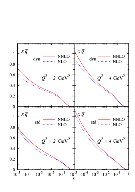
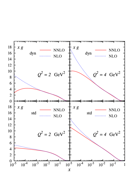
The sea and gluon distributions resulting from both fits are shown in Figures 1 and 2 respectively. The dynamical NLO sea distribution has a rather similar small–$x$ dependence as the standard one [4, 7]; this is caused by the fact that the valence–like sea input in (LABEL:eq:input) vanishes very slowly as $x\to 0$ (corresponding to a small value of $a_{\bar{q}}$, $a_{\bar{q}}\simeq 0.05$, according to Table 1) and thus is similarly increasing with decreasing $x$ down to $x\simeq 0.01$ as the sea input obtained by a standard fit. On the other hand, the dynamically generated NLO gluon is steeper as $x\to 0$ than the gluon distributions obtained from the standard fits. Similar remarks hold when comparing dynamical and standard distributions at NNLO. At NNLO the sea distribution $x\bar{q}$ is larger (steeper) than the NLO one, whereas the NNLO gluon distribution $xg$ is flatter as $x$ decreases and, in general, falls below the NLO one in the small–$x$ region. It is evident from Figure 2 that the NNLO gluon remains valencelike even at $Q^{2}=2-4$ GeV², i.e. decreases as $x$ decreases; this is mainly caused by the dominant NNLO gluon-gluon splitting function $P_{gg}^{(2)}$ which is negative and more singular as $x\to 0$ than the LO and NLO ones, $P_{gg}^{(2)}(x)\sim\frac{1}{x}\ln\frac{1}{x}$ [5].

Figure 3: The individual light ($u,d,s$) quark contribution $F_{L}^{q}$ to the total $F_{L}$ in (LABEL:eq:flms) in the dynamical (dyn) and standard (std) parton approach at NNLO and NLO for two representative low values of $Q^{2}$. The standard NLO results in the lower panel are similar for the CTEQ6 (anti)quark distributions [1]. Notice that, according to (LABEL:eq:flms), $F_{L}^{q}+F_{L}^{g}=F_{L}-F_{L}^{c}$.

Figure 4: As in Figure 3 but for the gluonic contribution $F_{L}^{g}$ to $F_{L}$ in (LABEL:eq:flms) with $F_{L}^{g}=\frac{2}{9}x\,C_{L,g}\otimes g$.

Figure 5: Dynamical parton model NNLO and NLO predictions for $F_{L}(x,Q^{2})$ in (LABEL:eq:flms).

Figure 6: As in Figure 5 but for the common standard parton distributions.

Figure 7: Our dynamical NNLO and NLO predictions for $F_{L}$ at a fixed value of $W=276$ GeV. The (partly preliminary) H1 data [30, 31, 45, 46] are at fixed $W\simeq 276$ GeV.

4 The longitudinal structure function $F_{L}(x,Q^{2})$

In this section we turn to the perturbative predictions for $F_{L}(x,Q^{2})$. Similarly to (1) one can write for $F_{L}$ in the $\overline{\rm MS}$ scheme,

$$x^{-1}F_{L} = C_{L,NS}\otimes q_{NS}$$

$$+\frac{2}{9}\,\left(C_{L,q}\otimes q_{S}+C_{L,g}\otimes g\right)\,+x^{-1}F_{L}^{c}$$

where again $\otimes$ in the $n_{f}=3$ light quark flavor sector denotes the convolution, $q_{NS}$ stands for the usual flavor non–singlet combination and $q_{S}=\sum_{q=u,d,s}(q+\bar{q})$ is the corresponding flavor–singlet quark distribution. We use the NLO expression [22, 23] for $F_{L}^{c}$ also in NNLO due to our ignorance of the ${\cal{O}}(\alpha_{s}^{3})$ NNLO heavy quark corrections. (Notice that $F_{L}^{c}$ is a genuinely subdominant NLO contribution to the total $F_{L}$, being less than 10% even at $Q^{2}=2$ GeV² and $x=10^{-5}$ and further decreases for increasing $x$. Furthermore, the NNLO 3–loop corrections to $F_{L}^{c}$ have been calculated recently [39] for $Q^{2}\gg m_{c}^{2}$, but this asymptotic result is neither applicable for our present investigation nor relevant for the majority of presently available data at lower values of $Q^{2}$.) The perturbative expansion of the coefficient functions can be written as

$$C_{L,i}(\alpha_{s},x)=\sum_{n=1}\,\left(\frac{\alpha_{s}(Q^{2})}{4\pi}\right)^{n}\,c_{L,i}^{(n)}(x)\,.$$ (7)

In LO, $c_{L,ns}^{(1)}=\frac{16}{3}x$, $c_{L,ps}^{(1)}=0$, $c_{L,g}^{(1)}=24x(1-x)$ and the singlet–quark coefficient function is decomposed into the non–singlet and a ‘pure singlet’ contribution, $c_{L,q}^{(n)}=c_{L,ns}^{(n)}+c_{L,ps}^{(n)}$. Sufficiently accurate simplified expressions for the exact [40, 41, 42] NLO and [43] NNLO coefficient functions $c_{L,i}^{(2)}$ and $c_{L,i}^{(3)}$, respectively, have been given in [8]. It has been furthermore noted in [8] that especially for $C_{L,g}$ both the NLO and NNLO contributions are rather large over almost the entire $x$–range. Most striking, however, is the behavior of both $C_{L,q}$ and $C_{L,g}$ at very small values [8, 44] of $x$: the vanishingly small LO parts ($xc_{L,i}^{(1)}\sim x^{2}$) are negligible as compared to the (negative) constant NLO 2–loop terms, which in turn are completely overwhelmed by the positive NNLO 3-loop singular corrections $xc_{L,i}^{(3)}\sim-\ln x$. This latter singular contribution might be indicative for the perturbative instability at NNLO [8], as discussed at the beginning, but it should be kept in mind that a small–$x$ information alone is insufficient for reliable estimates of the convolutions occurring in (LABEL:eq:flms) when evaluating physical observables.

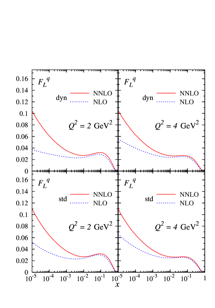
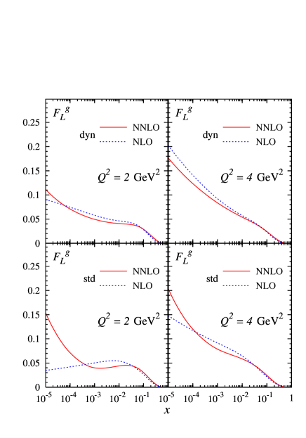
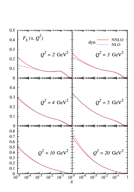
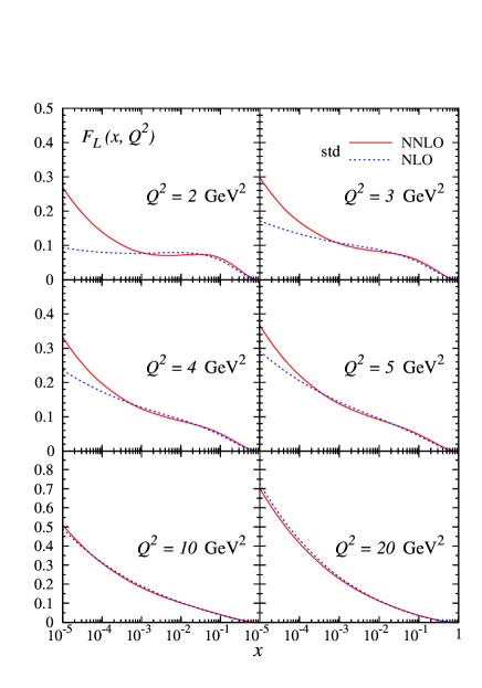
We display the predictions for the convolutions of the individual light $u,d,s$ quark ($F_{L}^{q}$) and gluon ($F_{L}^{g}$) contributions in (LABEL:eq:flms) in Figures 3 and 4, respectively, at two characteristic low values of $Q^{2}$. (Note that $F_{L}^{q}+F_{L}^{g}=F_{L}-F_{L}^{c}$ according to (LABEL:eq:flms)). Although the perturbative instability of the subdominant quark contribution in Figure 3 as obtained in a standard fit does not improve for the dynamical (sea) quark distributions, the instability disappears almost entirely for the dominant dynamical gluon contribution already at $Q^{2}\simeq 2$ GeV² as shown in Figure 4. This implies that the dynamical predictions for the total $F_{L}(x,Q^{2})$ become perturbatively stable already at the relevant low values of $Q^{2}$ $\stackrel{{\scriptstyle>}}{{\sim}}$ ${\cal{O}}(2-3$ GeV${}^{2})$ as evident from Figure 5, in contrast to the standard results in Figure 6. In the latter case the stability has not been fully reached even at $Q^{2}=5$ GeV² where the NNLO result at $x=10^{-5}$ is more than 20% larger than the NLO one. A similar discrepancy prevails for the dynamical predictions in Figure 5 at $Q^{2}=2$ GeV². This is, however, not too surprising since $Q^{2}=2$ GeV² represents somehow a borderline value for the leading twist–2 contribution to become dominant at small $x$ values. This is further corroborated by the observation that the dynamical NLO twist–2 fit slightly undershoots the HERA data for $F_{2}$ at $Q^{2}\simeq 2$ GeV² in the small–$x$ region (cf. Figure 1 of [4]), which indicates that nonperturbative (higher twist) contributions to $F_{2}$ become relevant for $Q^{2}$ $\stackrel{{\scriptstyle<}}{{\sim}}$ 2 GeV² [3, 4]. The NLO/NNLO instabilities implied by the standard fit results obtained in [2, 9] at $Q^{2}$ $\stackrel{{\scriptstyle<}}{{\sim}}$ 5 GeV² are even more violent than the ones shown in Figure 6. This is mainly due to the negative longitudinal cross section (negative $F_{L}(x,Q^{2})$) encountered in [2, 9]. The perturbative stability in any scenario becomes in general better the larger $Q^{2}$, typically beyond 5 GeV² [8, 2, 9], as shown in Figures 5 and 6. This is due to the fact that the $Q^{2}$–evolutions eventually force any parton distribution to become sufficiently steep in $x$.

For completeness we finally compare in Figure 7 our dynamical (leading twist) NNLO and NLO predictions for $F_{L}(x,Q^{2})$ with a representative selection of (partly preliminary) HERA–H1 data [30, 31, 45, 46]. Our results for $F_{L}$, being gluon dominated in the small–$x$ region, are in full agreement with present measurements which is in contrast to expectations [2, 9] based on negative parton distributions and structure functions at small values of $x$. To illustrate the manifest positive definiteness of our dynamically generated structure functions at $Q^{2}\geq\mu^{2}=0.5$ GeV² we show $F_{L}(x,Q^{2})$ in Figure 7 down to small values of $Q^{2}$ although leading twist–2 predictions need not necessarily be confronted with data below, say, 2 GeV². As pointed out in [5], where also a study on the $\pm 1\sigma$ uncertainty bands of $F_{L}$ has been performed, future precision measurements of $F_{L}$ could even distinguish between NLO results and NNLO effects in the very small–$x$ region.

5 Summary and conclusions

To summarize, recent deep inelastic data for the structure function $F_{2}^{p,n}$, without the inclusion of any $F_{L}$ data, have been analyzed in the dynamical and standard parton model approach at NLO and NNLO of perturbative QCD. In both approaches, perturbative QCD evolutions of parton distributions in the (very) small-$x$ region are fully compatible with all high-statistics measurements of the $Q^{2}$-dependence of $F_{2}(x,Q^{2})$ in that region. The results turned out to be perturbatively stable, therefore additional model assumptions concerning further resummations of subleading small-$x$ logarithms are not required.

Furthermore, the extracted parton distributions have been used to predict $F_{L}$. It has been shown that the extreme perturbative NNLO/NLO instability of $F_{L}$ at low $Q^{2}$, noted in [2, 9, 10], is an artifact of the commonly utilized ‘standard’ gluon distributions rather than an indication of a genuine problem of perturbative QCD. In fact it has been demonstrated that these extreme instabilities are reduced considerably already at $Q^{2}=2-3$ GeV² when utilizing the appropriate, dynamically generated, parton distributions at NLO and NNLO. It is interesting to notice, once again, the advantage of the dynamical parton model approach to perturbative QCD.

References

- [1] J. Pumplin et al., CTEQ Collab., JHEP 07 (2002) 012.
- [2] A.D. Martin et al., Phys. Lett. B 531 (2002) 216.
- [3] M. Glück, E. Reya, A. Vogt, Eur. Phys. J. C 5 (1998) 461.
- [4] M. Glück, P. Jimenez–Delgado, E. Reya, Eur. Phys. J. C 53 (2008) 355.
- [5] P. Jimenez-Delgado, E. Reya, arXiv:0810.4274 [hep-ph].
- [6] M. Glück, C. Pisano, E. Reya, Phys. Rev. D 77 (2008) 074002 [Erratum-ibid. D 78 (2008) 019902].
- [7] M. Glück, C. Pisano, E. Reya, Eur. Phys. J. C 50 (2007) 29.
- [8] S. Moch, J.A.M. Vermaseren, A. Vogt, Phys. Lett. B 606 (2005) 123, and references therein.
- [9] A.D. Martin, W.J. Stirling, R.S. Thorne, Phys. Lett. B 635 (2006) 305.
- [10] R.S. Thorne, Proceedings of the Ringberg Workshop on ‘New Trends in HERA Physics’ (Tegernsee, Oct. 2005), p. 359 (hep–ph/0511351).
- [11] C.D. White, R.S. Thorne, Phys. Rev. D 75 (2007) 034005.
- [12] M. Glück, E. Reya, Mod. Phys. Lett. A 22 (2007) 351.
- [13] W.L. van Neerven, A. Vogt, Nucl. Phys. B 568 (2000) 263.
- [14] W.L. van Neerven, A. Vogt, Nucl. Phys. B 588 (2000) 345 and arXiv:hep-ph/0006154 (corrected).
- [15] J. Blümlein, A. Vogt, Phys. Rev. D 58 (1998) 014020.
- [16] W. Furmanski, R. Petronzio, Z. Phys. C 11 (1982) 293, and references therein.
- [17] S. Moch, J.A.M. Vermaseren, A. Vogt, Nucl. Phys. B 688 (2004) 101.
- [18] M. Glück, E. Reya, C. Schuck, Nucl. Phys. B 754 (2006) 178.
- [19] A. Vogt, S. Moch, J.A.M. Vermaseren, Nucl. Phys. B 691 (2004) 129.
- [20] A. Vogt, Comput. Phys. Commun. 170 (2005) 65.
- [21] M. Glück, C. Pisano, E. Reya, Eur. Phys. J. C 40 (2005) 515.
- [22] E. Laenen, S. Riemersma, J. Smith, W.L. van Neerven, Nucl. Phys. B 392 (1993) 162.
- [23] S. Riemersma, J. Smith, W.L. van Neerven, Phys. Lett. B 347 (1995) 143.
- [24] M. Glück, E. Reya, M. Stratmann, Nucl. Phys. B 422 (1994) 37.
- [25] M. Glück, E. Reya, A. Vogt, Z. Phys. C 67 (1995) 433.
- [26] A. Vogt, DESY 96-012, Proc. of DIS ’96, Rome, April 1996, ed. by G. D’Agostini, A. Nigro (World Scientific, 1997) p. 254, hep-ph/9601352.
- [27] S.I. Alekhin, Phys. Rev. D 68 (2003) 014002.
- [28] S.I. Alekhin, JETP Lett. 82 (2005) 628.
- [29] S.I. Alekhin, K. Melnikov, F. Petriello, Phys. Rev. D 74 (2006) 054033.
- [30] C. Adloff et al., H1 Collab., Eur. Phys. J. C 21 (2001) 33.
- [31] C. Adloff et al., H1 Collab., Eur. Phys. J. C 30 (2003) 1.
- [32] A.C. Benvenuti et al., BCDMS Collab., Phys. Lett. B 223 (1989) 485; B 237 (1990) 599.
- [33] M. Arneodo et al., NMC Collab., Nucl. Phys. B 483 (1997) 3; B 487 (1997) 3.
- [34] A.L. Kataev et al., Phys. Lett. B 388 (1996) 179; B 417 (1998) 374.
- [35] J. Blümlein, H. Böttcher, A. Guffanti, Nucl. Phys. B (Proc. Suppl.) 135 (2004) 152; Nucl. Phys. B 774 (2007) 182.
- [36] W.K. Tung et al., CTEQ Collab., JHEP 02 (2007) 053.
- [37] J. Blümlein, DIS 2007 (Munich, April 2007), arXiv:0706.2430.
- [38] S. Forte, G. Altarelli, R.D. Ball, talk presented at DIS 2006, Tsukuba, Japan (April 2006), and references therein (arXiv:hep-ph/0606323).
- [39] J. Blümlein et al., Nucl. Phys. B 755 (2006) 272.
- [40] D.I. Kazakov, A.V. Kotikov, Nucl. Phys. B 307 (1988) 721 [Erratum-ibid. B 345 (1990) 299].
- [41] J. Sanchez Guillen et al., Nucl. Phys. B 353 (1991) 337.
- [42] E.B. Zijlstra, W.L. van Neerven, Phys. Lett. B 273 (1991) 476.
- [43] J.A.M. Vermaseren, A. Vogt, S. Moch, Nucl. Phys. B 724 (2005) 3.
- [44] S. Catani, F. Hautmann, Nucl. Phys. B 427 (1994) 475.
- [45] C. Adloff et al., H1 Collab., Phys. Lett. B 393 (1997) 452.
-
[46]
E.M. Lobodzinska, H1 Collab., DIS 2004
(Strbske Pleso, Slovakia),
hep–ph/0311180;
T. Lastovicka, H1 Collab., Eur. Phys. J. C 33 (2004) s388.