Neutrino mass matrix in triplet Higgs models with A4subscript𝐴4A_{4} symmetry

Myoung Chu Oha111mcoh73@gmail.com,   Seungwon Baekb222sbaek@korea.ac.kr

a Department of Physics, University of Seoul, Seoul 130-743, Republic of Korea
b The Institute of Basic Science and Department of Physics, Korea University, Seoul 136-701, Republic of Korea

Abstract

We consider triplet Higgs model with A4subscript𝐴4A_{4} symmetry to generate the neutrino mass matrix. The tribimaximal form of the neutrino mixing matrix can be naturally obtained. Imposing the neutrino oscillation data, we show that 1) both normal and inverted mass hierarchy are allowed, 2) there is a lower bound on the lightest neutrino mass and the effective mass for neutrinoless double beta decay, 3) the non-vanishing θ13subscript𝜃13\theta_{13} can be accommodated by considering small perturbation, 4) θatmsubscript𝜃atm\theta_{\rm atm} should be very close to π/4𝜋4\pi/4 even after perturbation.

1 Introduction

During last decade we have seen the firm evidences that the neutrinos have masses and mixings which may indicate the new physics (NP) beyond the Standard Model (SM). The solar, atmospheric and reactor neutrino experiments have measured the mass squared differences and mixing angles [1] as shown in Table 1.

Parameter Best fit 3-σ𝜎\sigma c.l. range
Δm2(105eV2)Δsubscriptsuperscript𝑚2direct-productsuperscript105superscripteV2\Delta m^{2}_{\odot}(10^{-5}{\rm eV}^{2}) (7.650.20+0.23)subscriptsuperscript7.650.230.20(7.65^{+0.23}_{-0.20}) 7.05 – 8.34
Δmatm2(103eV2)Δsubscriptsuperscript𝑚2atmsuperscript103superscripteV2\Delta m^{2}_{\rm atm}(10^{-3}{\rm eV}^{2}) (2.400.11+0.12)subscriptsuperscript2.400.120.11(2.40^{+0.12}_{-0.11}) 2.07 – 2.75
sin2(θ)superscript2subscript𝜃direct-product\sin^{2}(\theta_{\odot}) 0.3040.016+0.022subscriptsuperscript0.3040.0220.0160.304^{+0.022}_{-0.016} 0.25–0.37
sin2(θatm)superscript2subscript𝜃atm\sin^{2}(\theta_{\rm atm}) 0.500.06+0.07subscriptsuperscript0.500.070.060.50^{+0.07}_{-0.06} 0.36 – 0.67
sin2(θ13)superscript2subscript𝜃13\sin^{2}(\theta_{13}) 0.010.011+0.016subscriptsuperscript0.010.0160.0110.01^{+0.016}_{-0.011} \leq 0.056
Table 1: The neutrino oscillation data.

From the data in Table 1 only, we do not know the mass hierarchy, the absolute neutrino masses, or whether neutrinos are Majorana or Dirac particles. The future experiments like the neutrinoless double beta decay or Tritium decay may give further information on the nature of neutrinos. Therefore, it is important to get a model which predicts the mass matrix of neutrinos.

The current experimental data for the neutrino oscillations suggest that the mixing matrix, the Pontecorvo-Maki-Nakagawa-Sakata (MNS) matrix, is tribimaximal at the zeroth order [2]:

(|Ulν|2)=(2/31/301/61/31/21/61/31/2).superscriptsubscript𝑈𝑙𝜈223130161312161312\displaystyle(|U_{l\nu}|^{2})=\left(\begin{array}[]{ccc}2/3&1/3&0\\ 1/6&1/3&1/2\\ 1/6&1/3&1/2\end{array}\right). (4)

One of natural flavor symmetries which give the tribimaximal MNS matrix is the A4subscript𝐴4A_{4} symmetry [3, 4]. In addition, it was shown that the effective mass parameter relevant to the neutrinoless double beta decay can be predicted in a model with A4subscript𝐴4A_{4} flavor symmetry [4]. The tribimaximal mixing can also be naturally realized in the triplet Higgs model.

The triplet Higgs model, a TeV scale NP model, can generate Majorana neutrino masses. With A4subscript𝐴4A_{4} symmetry the Higgs triplet model naturally gives tribimaximal mixings to neutrinos. The predicted doubly charged Higgs (H±±superscript𝐻plus-or-minusabsentplus-or-minusH^{\pm\pm}), if light, can be found in the CERN Large Hadron Collider (LHC) experiment [5].

In this Letter we study a triplet Higgs model with A4subscript𝐴4A_{4} flavor symmetry which predicts not only the neutrinoless double beta decay but also all the neutrino masses. The Letter is organized as follows: In Section 2 we introduce our model. The numerical analysis for the neutrino masses and mixings and the predictions for the neutrinoless double beta decay are done in Section 3. We conclude in Section 4.

2 The Higgs triplet model with A4subscript𝐴4A_{4} symmetry

The conventional method to generate the neutrino masses is to introduce the heavy Majorana right-handed neutrinos (type-I seesaw). However, it is difficult to test this case experimentally. An alternative way to give Majorana masses to neutrinos is to introduce SU(2)L𝑆𝑈subscript2𝐿SU(2)_{L} Higgs triplet ΔΔ\Delta with U(1)Y𝑈subscript1𝑌U(1)_{Y} charge 1 in the SM (type-II seesaw) [8]. Via Yukawa interaction the Higgs triplet model can provide Majorana masses to neutrinos if the neutral component Δ0superscriptΔ0\Delta^{0} gets very small vev [7]. The Yukawa interaction is given by

Ysubscript𝑌\displaystyle{\cal L}_{Y} =\displaystyle= 12hijLiTCiτ2ΔLj+H.c,formulae-sequence12subscript𝑖𝑗superscriptsubscript𝐿𝑖𝑇𝐶𝑖subscript𝜏2Δsubscript𝐿𝑗𝐻𝑐\displaystyle{1\over 2}h_{ij}L_{i}^{T}Ci\tau_{2}\Delta L_{j}+H.c, (5)

where hijsubscript𝑖𝑗h_{ij} is a complex symmetric coupling matrix, Li=(νi,li)LTsubscript𝐿𝑖subscriptsuperscriptsubscript𝜈𝑖subscript𝑙𝑖𝑇𝐿L_{i}=(\nu_{i},l_{i})^{T}_{L} is a left-handed lepton doublet, C𝐶C is the Dirac charge conjugation operator, and τ2subscript𝜏2\tau_{2} is a Pauli matrix. The Higgs triplet can be decomposed as follows:

Δ=(Δ+/2Δ++Δ0Δ+/2).ΔsuperscriptΔ2superscriptΔabsentsuperscriptΔ0superscriptΔ2\displaystyle\Delta=\left(\begin{array}[]{cc}\Delta^{+}/\sqrt{2}&\Delta^{++}\\ \Delta^{0}&-\Delta^{+}/\sqrt{2}\end{array}\right). (8)

Then the neutrino mass matrix is written in terms of the vev as

(Mν)ij=hijΔ0.subscriptsubscript𝑀𝜈𝑖𝑗subscript𝑖𝑗delimited-⟨⟩superscriptΔ0\displaystyle(M_{\nu})_{ij}=h_{ij}\langle\Delta^{0}\rangle. (9)

There are many attempts to obtain the form of neutrino mass matrix suggested by Table 1 in the framework of A4subscript𝐴4A_{4} symmetry in the literature [3, 4]. The group A4subscript𝐴4A_{4} has three singlet representations, 𝟏1{\bf 1}, 𝟏superscript1{\bf 1^{\prime}}, 𝟏′′superscript1′′{\bf 1^{\prime\prime}}, and a triplet representation, 𝟑3{\bf 3}. Their tensor products are decomposed as

𝟑𝟑=𝟑s𝟑a𝟏𝟏𝟏′′,𝟏𝟏′′=𝟏.formulae-sequencetensor-product33direct-sumsubscript3𝑠subscript3𝑎1superscript1superscript1′′tensor-productsuperscript1superscript1′′1\displaystyle{\bf 3}\otimes{\bf 3}={\bf 3}_{s}\oplus{\bf 3}_{a}\oplus{\bf 1}\oplus{\bf 1^{\prime}}\oplus{\bf 1^{\prime\prime}},\quad{\bf 1^{\prime}}\otimes{\bf 1^{\prime\prime}}={\bf 1}. (10)

For two vectors (x1,x2,x3)subscript𝑥1subscript𝑥2subscript𝑥3(x_{1},x_{2},x_{3}) and (y1,y2,y3)subscript𝑦1subscript𝑦2subscript𝑦3(y_{1},y_{2},y_{3}) transforming as 𝟑3{\bf 3}, the first rule in the above equation states that

(𝟑𝟑)𝟑ssubscripttensor-product33subscript3𝑠\displaystyle({\bf 3}\otimes{\bf 3})_{{\bf 3}_{s}} =\displaystyle= (x2y3+x3y2,x3y1+x1y3,x1y2+x2y1),subscript𝑥2subscript𝑦3subscript𝑥3subscript𝑦2subscript𝑥3subscript𝑦1subscript𝑥1subscript𝑦3subscript𝑥1subscript𝑦2subscript𝑥2subscript𝑦1\displaystyle(x_{2}y_{3}+x_{3}y_{2},x_{3}y_{1}+x_{1}y_{3},x_{1}y_{2}+x_{2}y_{1}),
(𝟑𝟑)𝟑asubscripttensor-product33subscript3𝑎\displaystyle({\bf 3}\otimes{\bf 3})_{{\bf 3}_{a}} =\displaystyle= (x2y3x3y2,x3y1x1y3,x1y2x2y1),subscript𝑥2subscript𝑦3subscript𝑥3subscript𝑦2subscript𝑥3subscript𝑦1subscript𝑥1subscript𝑦3subscript𝑥1subscript𝑦2subscript𝑥2subscript𝑦1\displaystyle(x_{2}y_{3}-x_{3}y_{2},x_{3}y_{1}-x_{1}y_{3},x_{1}y_{2}-x_{2}y_{1}),
(𝟑𝟑)𝟏subscripttensor-product331\displaystyle({\bf 3}\otimes{\bf 3})_{{\bf 1}} =\displaystyle= x1y1+x2y2+x3y3,subscript𝑥1subscript𝑦1subscript𝑥2subscript𝑦2subscript𝑥3subscript𝑦3\displaystyle x_{1}y_{1}+x_{2}y_{2}+x_{3}y_{3},
(𝟑𝟑)𝟏subscripttensor-product33superscript1\displaystyle({\bf 3}\otimes{\bf 3})_{{\bf 1^{\prime}}} =\displaystyle= x1y1+ωx2y2+ω2x3y3,subscript𝑥1subscript𝑦1𝜔subscript𝑥2subscript𝑦2superscript𝜔2subscript𝑥3subscript𝑦3\displaystyle x_{1}y_{1}+\omega x_{2}y_{2}+\omega^{2}x_{3}y_{3},
(𝟑𝟑)𝟏′′subscripttensor-product33superscript1′′\displaystyle({\bf 3}\otimes{\bf 3})_{{\bf 1^{\prime\prime}}} =\displaystyle= x1y1+ω2x2y2+ωx3y3.subscript𝑥1subscript𝑦1superscript𝜔2subscript𝑥2subscript𝑦2𝜔subscript𝑥3subscript𝑦3\displaystyle x_{1}y_{1}+\omega^{2}x_{2}y_{2}+\omega x_{3}y_{3}. (11)

We assign the three-dimensional representation 𝟑3{\bf 3} of A4subscript𝐴4A_{4} to the doublet Higgs ϕitalic-ϕ\phi and the triplet Higgs ΔΔ\Delta as in Table 2. To implement A4subscript𝐴4A_{4} flavor symmetric Lagrangian and get a neutrino mass matrix consistent with the experiments, we need to introduce additional Higgs multiplets. Here we introduce three more triplet Higgs χisubscript𝜒𝑖\chi_{i} (i=1,2,3)𝑖123(i=1,2,3) like [4], which are assigned 𝟏,𝟏,𝟏′′1superscript1superscript1′′{\bf 1},{\bf 1^{\prime}},{\bf 1^{\prime\prime}} of A4subscript𝐴4A_{4}. We assign 𝟏,𝟏,𝟏′′1superscript1superscript1′′{\bf 1},{\bf 1^{\prime}},{\bf 1^{\prime\prime}} to the right-handed leptons and 3 to the left-handed leptons.

Fields ecsuperscript𝑒𝑐e^{c} L𝐿L ϕitalic-ϕ\phi χ1subscript𝜒1\chi_{1} χ2subscript𝜒2\chi_{2} χ3subscript𝜒3\chi_{3} ΔΔ\Delta
A4subscript𝐴4A_{4} 𝟏,𝟏,𝟏′′1superscript1superscript1′′\bf{1},\bf{1^{\prime}},\bf{1^{\prime\prime}} 𝟑3\bf{3} 𝟑3\bf{3} 𝟏1\bf{1} 𝟏superscript1\bf{1^{\prime}} 𝟏′′superscript1′′\bf{1^{\prime\prime}} 𝟑3\bf{3}
SU(2)L𝑆𝑈subscript2𝐿SU(2)_{L} 𝟏1\bf{1} 𝟐2\bf{2} 𝟐2\bf{2} 𝟑3\bf{3} 𝟑3\bf{3} 𝟑3\bf{3} 𝟑3\bf{3}
U(1)Y𝑈subscript1𝑌U(1)_{Y} 111 1/212-1/2 1/2121/2 111 111 111 111
Table 2: The assignments of A4subscript𝐴4A_{4} and the SU(2)L×U(1)Y𝑆𝑈subscript2𝐿𝑈subscript1𝑌SU(2)_{L}\times U(1)_{Y} representations in our model.

Then not all the couplings in (5) but only the following A4subscript𝐴4A_{4}-symmetric Yukawa interactions are allowed:

\displaystyle{\cal L} =\displaystyle= λee¯R(ϕL)1λee′′¯R(ϕL)1λe′′e¯R(ϕL)1′′subscript𝜆𝑒subscript¯𝑒𝑅subscriptsuperscriptitalic-ϕ𝐿1subscriptsuperscript𝜆𝑒subscript¯superscript𝑒′′𝑅subscriptsuperscriptitalic-ϕ𝐿superscript1subscriptsuperscript𝜆′′𝑒subscript¯superscript𝑒𝑅subscriptsuperscriptitalic-ϕ𝐿superscript1′′\displaystyle-\lambda_{e}\overline{e}_{R}(\phi^{\dagger}L)_{1}-\lambda^{\prime}_{e}\overline{e^{\prime\prime}}_{R}(\phi^{\dagger}L)_{1^{\prime}}-\lambda^{\prime\prime}_{e}\overline{e^{\prime}}_{R}(\phi^{\dagger}L)_{1^{\prime\prime}} (12)
+12λΔLTCiτ2ΔL+12λ1(LTCiτ2χ1L)1+12λ2(LTCiτ2χ2L)1′′+12λ3(LTCiτ2χ3L)1,12subscript𝜆Δsuperscript𝐿𝑇𝐶𝑖subscript𝜏2Δ𝐿12subscript𝜆1subscriptsuperscript𝐿𝑇𝐶𝑖subscript𝜏2subscript𝜒1𝐿112subscript𝜆2subscriptsuperscript𝐿𝑇𝐶𝑖subscript𝜏2subscript𝜒2𝐿superscript1′′12subscript𝜆3subscriptsuperscript𝐿𝑇𝐶𝑖subscript𝜏2subscript𝜒3𝐿superscript1\displaystyle+{1\over 2}\lambda_{\Delta}L^{T}Ci\tau_{2}\Delta L+{1\over 2}\lambda_{1}(L^{T}Ci\tau_{2}\chi_{1}L)_{1}+{1\over 2}\lambda_{2}(L^{T}Ci\tau_{2}\chi_{2}L)_{1^{\prime\prime}}+{1\over 2}\lambda_{3}(L^{T}Ci\tau_{2}\chi_{3}L)_{1^{\prime}},

where the subscripts 1,1,1′′1superscript1superscript1′′1,1^{\prime},1^{\prime\prime} represent the transformation rules of the (ϕL)superscriptitalic-ϕ𝐿(\phi^{\dagger}L) pair in the first line and of the (LTL)superscript𝐿𝑇𝐿(L^{T}L) pair in the second line. The resulting lepton and neutrino mass matrices have the following form

Mlsubscript𝑀𝑙\displaystyle M_{l} =\displaystyle= (λev1λev2λev3λev1ωλev2ω2λev3λe′′v1ω2λe′′v2ωλe′′v3),subscript𝜆𝑒subscript𝑣1subscript𝜆𝑒subscript𝑣2subscript𝜆𝑒subscript𝑣3subscriptsuperscript𝜆𝑒subscript𝑣1𝜔subscriptsuperscript𝜆𝑒subscript𝑣2superscript𝜔2subscriptsuperscript𝜆𝑒subscript𝑣3subscriptsuperscript𝜆′′𝑒subscript𝑣1superscript𝜔2subscriptsuperscript𝜆′′𝑒subscript𝑣2𝜔subscriptsuperscript𝜆′′𝑒subscript𝑣3\displaystyle\left(\begin{array}[]{ccc}\lambda_{e}v_{1}&\lambda_{e}v_{2}&\lambda_{e}v_{3}\\ \lambda^{\prime}_{e}v_{1}&\omega\lambda^{\prime}_{e}v_{2}&\omega^{2}\lambda^{\prime}_{e}v_{3}\\ \lambda^{\prime\prime}_{e}v_{1}&\omega^{2}\lambda^{\prime\prime}_{e}v_{2}&\omega\lambda^{\prime\prime}_{e}v_{3}\end{array}\right), (16)
Mνsubscript𝑀𝜈\displaystyle M_{\nu} =\displaystyle= (a+b+cfefa+ω2b+ωcdeda+ωb+ω2c),𝑎𝑏𝑐𝑓𝑒𝑓𝑎superscript𝜔2𝑏𝜔𝑐𝑑𝑒𝑑𝑎𝜔𝑏superscript𝜔2𝑐\displaystyle\left(\begin{array}[]{ccc}a+b+c&f&e\\ f&a+\omega^{2}b+\omega c&d\\ e&d&a+\omega b+\omega^{2}c\end{array}\right), (20)

where vi=ϕi(i=1,2,3)subscript𝑣𝑖delimited-⟨⟩subscriptitalic-ϕ𝑖𝑖123v_{i}=\langle{\phi_{i}}\rangle\;(i=1,2,3) and

a=λ1χ10,b=λ2χ20,c=λ3χ30,formulae-sequence𝑎subscript𝜆1delimited-⟨⟩superscriptsubscript𝜒10formulae-sequence𝑏subscript𝜆2delimited-⟨⟩superscriptsubscript𝜒20𝑐subscript𝜆3delimited-⟨⟩superscriptsubscript𝜒30\displaystyle a=\lambda_{1}\langle{\chi_{1}^{0}}\rangle,\quad b=\lambda_{2}\langle{\chi_{2}^{0}}\rangle,\quad c=\lambda_{3}\langle{\chi_{3}^{0}}\rangle,
d=λΔΔ10,e=λΔΔ20,f=λΔΔ30.formulae-sequence𝑑subscript𝜆Δdelimited-⟨⟩superscriptsubscriptΔ10formulae-sequence𝑒subscript𝜆Δdelimited-⟨⟩superscriptsubscriptΔ20𝑓subscript𝜆Δdelimited-⟨⟩superscriptsubscriptΔ30\displaystyle d=\lambda_{\Delta}\langle{\Delta_{1}^{0}}\rangle,\quad e=\lambda_{\Delta}\langle{\Delta_{2}^{0}}\rangle,\quad f=\lambda_{\Delta}\langle{\Delta_{3}^{0}}\rangle. (21)

We assume v1=v2=v3subscript𝑣1subscript𝑣2subscript𝑣3v_{1}=v_{2}=v_{3}, and d=e=f𝑑𝑒𝑓d=e=f, which can be guaranteed by a residual symmetry like Z3subscript𝑍3Z_{3}. For simplicity we impose additional assumption: b=c𝑏𝑐b=c which naturally gives the maximal atmospheric neutrino mixing, although it is not required by any symmetry. It is straightforward to extend our analysis to the case bc𝑏𝑐b\not=c. We will consider the effect of small perturbation of cb𝑐𝑏c-b in Section 3.2.

Then the lepton mass matrix, Mlsubscript𝑀𝑙M_{l}, can be diagonalized by rotating the left-handed lepton by the unitary matrix

U(ω)=13(1111ωω21ω2ω).𝑈𝜔131111𝜔superscript𝜔21superscript𝜔2𝜔\displaystyle U(\omega)={1\over\sqrt{3}}\left(\begin{array}[]{ccc}1&1&1\\ 1&\omega&\omega^{2}\\ 1&\omega^{2}&\omega\end{array}\right). (25)

The neutrino mass matrix is diagonalized by the transformation

UνTMνUν=Mνdiag,superscriptsubscript𝑈𝜈𝑇subscript𝑀𝜈subscript𝑈𝜈superscriptsubscript𝑀𝜈diag\displaystyle U_{\nu}^{T}\,M_{\nu}\,U_{\nu}=M_{\nu}^{\rm diag}, (26)

where Uνsubscript𝑈𝜈U_{\nu} is a unitary matrix which can be decomposed into three successive rotation matrices: Uν=V23V13V12subscript𝑈𝜈subscript𝑉23subscript𝑉13subscript𝑉12U_{\nu}=V_{23}V_{13}V_{12} [1]. The form of the neutrino mass matrix when b=c𝑏𝑐b=c is given by

Mνsubscript𝑀𝜈\displaystyle M_{\nu} =\displaystyle= (a+2bdddabdddab).𝑎2𝑏𝑑𝑑𝑑𝑎𝑏𝑑𝑑𝑑𝑎𝑏\displaystyle\left(\begin{array}[]{ccc}a+2b&d&d\\ d&a-b&d\\ d&d&a-b\end{array}\right). (30)

The resulting MNS matrix is the product of U(ω)𝑈𝜔U(\omega) and Uνsubscript𝑈𝜈U_{\nu}:

UMNS=U(ω)Uν.subscript𝑈MNS𝑈𝜔subscript𝑈𝜈\displaystyle U_{\rm MNS}=U(\omega)\,U_{\nu}. (31)

Alternatively we can work in the basis where the mass matrix of the charged lepton is diagonal. In this basis the neutrino mass matrix is in the form:

Mνeffsuperscriptsubscript𝑀𝜈eff\displaystyle M_{\nu}^{\rm eff} =\displaystyle= U(ω)MνU(ω)=(a+2dbbbbadbadb),𝑈superscript𝜔subscript𝑀𝜈𝑈superscript𝜔𝑎2𝑑𝑏𝑏𝑏𝑏𝑎𝑑𝑏𝑎𝑑𝑏\displaystyle U(\omega)^{*}M_{\nu}U(\omega)^{\dagger}=\left(\begin{array}[]{ccc}a+2d&b&b\\ b&b&a-d\\ b&a-d&b\end{array}\right), (35)

such that

UMNSTMνeffUMNS=Mνdiag.superscriptsubscript𝑈MNS𝑇superscriptsubscript𝑀𝜈effsubscript𝑈MNSsuperscriptsubscript𝑀𝜈diag\displaystyle U_{\rm MNS}^{T}M_{\nu}^{\rm eff}U_{\rm MNS}=M_{\nu}^{\rm diag}. (36)

Since the neutrino mass matrix is symmetric under the exchange of νμντsubscript𝜈𝜇subscript𝜈𝜏\nu_{\mu}\leftrightarrow\nu_{\tau}, we get a bimaximal 23232-3 mixing and a vanishing 13131-3 mixing

θ23=π/4,θ13=0.formulae-sequencesubscript𝜃23𝜋4subscript𝜃130\displaystyle\theta_{23}=\pi/4,\quad\theta_{13}=0. (37)

The (35) does not automatically generate the desired mixing angle θ12subscript𝜃12\theta_{12} for the tribimaximal mixing matrix. The form of (4), however, can be achieved in a wide region of parameter space. This can be seen from the fact that the UMNSsubscript𝑈MNSU_{\rm MNS} obtained in (36) can be decomposed in general as

UMNS=diag(eiβ1,eiβ2,eiβ3)UMNSstP(β)UMNSst,subscript𝑈MNSdiagsuperscript𝑒𝑖subscript𝛽1superscript𝑒𝑖subscript𝛽2superscript𝑒𝑖subscript𝛽3superscriptsubscript𝑈MNSst𝑃𝛽superscriptsubscript𝑈MNSst\displaystyle U_{\rm MNS}={\rm diag}(e^{i\beta_{1}},e^{i\beta_{2}},e^{i\beta_{3}})\;U_{\rm MNS}^{\rm st}\equiv P(\beta)U_{\rm MNS}^{\rm st}, (38)

where UMNSstsuperscriptsubscript𝑈MNSstU_{\rm MNS}^{\rm st} is the physically measurable matrix which includes the Majorana phases in the standard form [1],

UMNSst=(c12c13s12c13s13eiδs12c23c12s23s13eiδc12c23s12s23s13eiδs23c13s12s23c12c23s13eiδc12s23s12c23s13eiδc23c13)×diag(eiα1,eiα2,1).superscriptsubscript𝑈MNSstmatrixsubscript𝑐12subscript𝑐13subscript𝑠12subscript𝑐13subscript𝑠13superscript𝑒𝑖𝛿subscript𝑠12subscript𝑐23subscript𝑐12subscript𝑠23subscript𝑠13superscript𝑒𝑖𝛿subscript𝑐12subscript𝑐23subscript𝑠12subscript𝑠23subscript𝑠13superscript𝑒𝑖𝛿subscript𝑠23subscript𝑐13subscript𝑠12subscript𝑠23subscript𝑐12subscript𝑐23subscript𝑠13superscript𝑒𝑖𝛿subscript𝑐12subscript𝑠23subscript𝑠12subscript𝑐23subscript𝑠13superscript𝑒𝑖𝛿subscript𝑐23subscript𝑐13diagsuperscript𝑒𝑖subscript𝛼1superscript𝑒𝑖subscript𝛼21\displaystyle U_{\rm MNS}^{\rm st}=\left(\matrix{\phantom{-}c_{12}c_{13}&s_{12}c_{13}&s_{13}e^{-i\delta}\cr-s_{12}c_{23}-c_{12}s_{23}s_{13}e^{i\delta}&\phantom{-}c_{12}c_{23}-s_{12}s_{23}s_{13}e^{i\delta}&s_{23}c_{13}\cr\phantom{-}s_{12}s_{23}-c_{12}c_{23}s_{13}e^{i\delta}&-c_{12}s_{23}-s_{12}c_{23}s_{13}e^{i\delta}&c_{23}c_{13}}\right)\times{\rm diag}(e^{i\alpha_{1}},~{}e^{i\,\alpha_{2}},~{}1). (39)

The phase matrix, P(β)𝑃𝛽P(\beta), in (38) can be absorbed into the right-handed charged lepton sector, and therefore, is unphysical. However, since the Mνeffsuperscriptsubscript𝑀𝜈effM_{\nu}^{\rm eff} is complex matrix in general, the phase matrix P(β)𝑃𝛽P(\beta) is generally allowed, and it makes the allowed parameter space much more wider than the real matrix case. The condition for the tribimaximal mixing including the unphysical β𝛽\beta’s can be written as

d=(eiβ1eiβ2)[a(eiβ1+eiβ2)+beiβ2)]2e2iβ1+e2iβ2,\displaystyle d=-\frac{(e^{i\beta_{1}}-e^{i\beta_{2}})[a(e^{i\beta_{1}}+e^{i\beta_{2}})+be^{i\beta_{2}})]}{2e^{2i\beta_{1}}+e^{2i\beta_{2}}}, (40)

where the phases β1,β2subscript𝛽1subscript𝛽2\beta_{1},\beta_{2} can take arbitrary values. The d=0𝑑0d=0 is a special case to give the tribimaximal mixing matrix.

We note that if we assume Δ20=Δ30=0delimited-⟨⟩superscriptsubscriptΔ20delimited-⟨⟩superscriptsubscriptΔ300\langle{\Delta_{2}^{0}}\rangle=\langle{\Delta_{3}^{0}}\rangle=0, the tribimaximal form can be obtained without further conditions among a,b,d𝑎𝑏𝑑a,b,d. This case was considered in [6].

Our model is similar to the one considered in [4]. But their neutrino mass matrix is different from ours and can be obtained by exchanging bd𝑏𝑑b\leftrightarrow d. Phenomenologically the two are significantly different in that, for example, d=0𝑑0d=0 gives the tribimaximal mixing matrix in our case, while the model in [4] cannot.

3 The numerical analysis and model predictions

3.1 The case b=c𝑏𝑐b=c

As mentioned in the previous section, we get θ23=π/4,θ13=0formulae-sequencesubscript𝜃23𝜋4subscript𝜃130\theta_{23}=\pi/4,\theta_{13}=0 in this case. More explicitly, with UMNS=U23U13U12subscript𝑈MNSsubscript𝑈23subscript𝑈13subscript𝑈12U_{\rm MNS}=U_{23}U_{13}U_{12}, we get

U23=(1000121201212),U13=(100010001).formulae-sequencesubscript𝑈23matrix1000121201212subscript𝑈13matrix100010001\displaystyle U_{23}=\left(\matrix{1&0&0\cr 0&{1\over\sqrt{2}}&-{1\over\sqrt{2}}\cr 0&{1\over\sqrt{2}}&\phantom{-}{1\over\sqrt{2}}}\right),\quad U_{13}=\left(\matrix{1&0&0\cr 0&1&0\cr 0&0&1}\right). (41)

After rotating in the 232323 and 131313 plane, we can block-diagonalize the Mνeffsuperscriptsubscript𝑀𝜈effM_{\nu}^{\rm eff} as

UMNSTMνeffUMNS=U12T(a+2d2b02ba+bd000a+b+d)U12=Mνdiag.superscriptsubscript𝑈MNS𝑇superscriptsubscript𝑀𝜈effsubscript𝑈MNSsuperscriptsubscript𝑈12𝑇matrix𝑎2𝑑2𝑏02𝑏𝑎𝑏𝑑000𝑎𝑏𝑑subscript𝑈12superscriptsubscript𝑀𝜈diag\displaystyle U_{\rm MNS}^{T}M_{\nu}^{\rm eff}U_{\rm MNS}=U_{12}^{T}\;\left(\matrix{a+2d&\sqrt{2}b&0\cr\sqrt{2}b&a+b-d&0\cr 0&0&-a+b+d}\right)\;U_{12}=M_{\nu}^{\rm diag}. (42)

We can read m32=|a+b+d|2superscriptsubscript𝑚32superscript𝑎𝑏𝑑2m_{3}^{2}=|-a+b+d|^{2} and obtain the remaining mass-squared eigenvalues, m12,m22superscriptsubscript𝑚12superscriptsubscript𝑚22m_{1}^{2},m_{2}^{2}, and the remaining mixing angle, θ12subscript𝜃12\theta_{12}, by squaring (42), i.e. UMNSMνeffMνeffUMNS=(Mνdiag)2superscriptsubscript𝑈MNSsuperscriptsuperscriptsubscript𝑀𝜈effsuperscriptsubscript𝑀𝜈effsubscript𝑈MNSsuperscriptsuperscriptsubscript𝑀𝜈diag2U_{\rm MNS}^{\dagger}{M_{\nu}^{\rm eff}}^{\dagger}M_{\nu}^{\rm eff}U_{\rm MNS}=\left(M_{\nu}^{\rm diag}\right)^{2}. There can be spontaneous CP violation and the parameters a,b,d𝑎𝑏𝑑a,b,d are in general complex numbers: a=|a|eiφa,b=|b|eiφbformulae-sequence𝑎𝑎superscript𝑒𝑖subscript𝜑𝑎𝑏𝑏superscript𝑒𝑖subscript𝜑𝑏a=|a|e^{i\varphi_{a}},b=|b|e^{i\varphi_{b}}, and d=|d|eiφd𝑑𝑑superscript𝑒𝑖subscript𝜑𝑑d=|d|e^{i\varphi_{d}}. However, one of the vev’s can be made real by SU(2)𝑆𝑈2SU(2) rotation. So we can set φd0subscript𝜑𝑑0\varphi_{d}\equiv 0 without loss of generality. Then it is straightforward to get the mixing angle θ12subscript𝜃12\theta_{12} of U12subscript𝑈12U_{12} and the mass-squared eigenvalues:

m1,22superscriptsubscript𝑚122\displaystyle m_{1,2}^{2} =\displaystyle= |d|22|ΛΔ|,superscript𝑑22minus-or-plusΛΔ\displaystyle{|d|^{2}\over 2}|\Lambda\mp\Delta|,
m32superscriptsubscript𝑚32\displaystyle m_{3}^{2} =\displaystyle= |d|2(x2+y2+12xycosφab2xcosφa+2ycosφb),superscript𝑑2superscript𝑥2superscript𝑦212𝑥𝑦subscript𝜑𝑎𝑏2𝑥subscript𝜑𝑎2𝑦subscript𝜑𝑏\displaystyle|d|^{2}\left(x^{2}+y^{2}+1-2xy\cos\varphi_{ab}-2x\cos\varphi_{a}+2y\cos\varphi_{b}\right),
t12subscript𝑡12\displaystyle t_{12} \displaystyle\equiv tanθ12=Δ+ΣΔΣ,subscript𝜃12ΔΣΔΣ\displaystyle\tan{\theta_{12}}=\sqrt{\Delta+\Sigma\over\Delta-\Sigma}, (43)

where x|a|/|d|𝑥𝑎𝑑x\equiv|a|/|d|, y|b|/|d|𝑦𝑏𝑑y\equiv|b|/|d|, φabφaφbsubscript𝜑𝑎𝑏subscript𝜑𝑎subscript𝜑𝑏\varphi_{ab}\equiv\varphi_{a}-\varphi_{b} and

ΛΛ\displaystyle\Lambda =\displaystyle= 2x2+5y2+5+2xycosφab+2xcosφa2ycosφb,2superscript𝑥25superscript𝑦252𝑥𝑦subscript𝜑𝑎𝑏2𝑥subscript𝜑𝑎2𝑦subscript𝜑𝑏\displaystyle 2x^{2}+5y^{2}+5+2xy\cos\varphi_{ab}+2x\cos\varphi_{a}-2y\cos\varphi_{b},
ΣΣ\displaystyle\Sigma =\displaystyle= y2+32xycosφab+6xcosφa+2ycosφb,superscript𝑦232𝑥𝑦subscript𝜑𝑎𝑏6𝑥subscript𝜑𝑎2𝑦subscript𝜑𝑏\displaystyle-y^{2}+3-2xy\cos\varphi_{ab}+6x\cos\varphi_{a}+2y\cos\varphi_{b},
ΔΔ\displaystyle\Delta =\displaystyle= Σ2+8(ϵ12+ϵ22),superscriptΣ28superscriptsubscriptitalic-ϵ12superscriptsubscriptitalic-ϵ22\displaystyle\sqrt{\Sigma^{2}+8(\epsilon_{1}^{2}+\epsilon_{2}^{2})}, (44)

where ϵ1=y2+2xycosφab+ycosφbsubscriptitalic-ϵ1superscript𝑦22𝑥𝑦subscript𝜑𝑎𝑏𝑦subscript𝜑𝑏\epsilon_{1}=y^{2}+2xy\cos\varphi_{ab}+y\cos\varphi_{b} and ϵ2=3ysinφbsubscriptitalic-ϵ23𝑦subscript𝜑𝑏\epsilon_{2}=3y\sin\varphi_{b}.

We can show that ΛΔΛΔ\Lambda\geq\Delta (the equality sign holds for x=27/32,y=(914641)/128formulae-sequence𝑥2732𝑦914641128x=27/32,y=(91-\sqrt{4641})/128, and φa=φb=0subscript𝜑𝑎subscript𝜑𝑏0\varphi_{a}=\varphi_{b}=0 ). So the smallness of the solar mass difference, Δm2=Δm212=|d|2ΔΔsubscriptsuperscript𝑚2direct-productΔsuperscriptsubscript𝑚212superscript𝑑2Δ\Delta m^{2}_{\odot}=\Delta m_{21}^{2}=|d|^{2}\Delta, implies Δ0Δ0\Delta\approx 0. And this leads to Σϵ1ϵ20Σsubscriptitalic-ϵ1subscriptitalic-ϵ20\Sigma\approx\epsilon_{1}\approx\epsilon_{2}\approx 0. From this we get a “magic relation” for y=𝒪(1)𝑦𝒪1y={\cal O}(1):

φb0,y+2xcosφa+10,formulae-sequencesubscript𝜑𝑏0𝑦2𝑥subscript𝜑𝑎10\displaystyle\varphi_{b}\approx 0,\quad y+2x\cos\varphi_{a}+1\approx 0, (45)
oror\displaystyle{\rm or} φbπ,y2xcosφa10.formulae-sequencesubscript𝜑𝑏𝜋𝑦2𝑥subscript𝜑𝑎10\displaystyle\varphi_{b}\approx\pi,\quad y-2x\cos\varphi_{a}-1\approx 0.

We note that the above conditions give Δ3ΣΔ3Σ\Delta\approx-3\Sigma or tanθ12=1/2subscript𝜃1212\tan\theta_{12}=1/\sqrt{2}. Then we obtain the tribimaximal mixing (4) without further conditions333If (45) holds exactly, t12subscript𝑡12t_{12} becomes undetermined. . Although the magic relation (45) is not guaranteed by any symmetry, it is satisfied in a large parameter space, especially when the CP violating phase φasubscript𝜑𝑎\varphi_{a} is allowed. In this approximation we get the following mass-squared differences:

Δm212Δsuperscriptsubscript𝑚212\displaystyle\Delta m_{21}^{2} \displaystyle\equiv m22m12|d|2Δ,superscriptsubscript𝑚22superscriptsubscript𝑚12superscript𝑑2Δ\displaystyle m_{2}^{2}-m_{1}^{2}\approx|d|^{2}\Delta,
Δm322Δsuperscriptsubscript𝑚322\displaystyle\Delta m_{32}^{2} \displaystyle\equiv m32m226|d|2y(forφb=0),or6|d|2y(forφb=π).superscriptsubscript𝑚32superscriptsubscript𝑚226superscript𝑑2𝑦forsubscript𝜑𝑏0or6superscript𝑑2𝑦forsubscript𝜑𝑏𝜋\displaystyle m_{3}^{2}-m_{2}^{2}\approx 6|d|^{2}y\;({\rm for}\;\varphi_{b}=0),\;\;{\rm or}\;\;-6|d|^{2}y\;({\rm for}\;\varphi_{b}=\pi). (46)

Here Δm212>0Δsuperscriptsubscript𝑚2120\Delta m_{21}^{2}>0 by definition and it can be identified with the Δmsol2Δsuperscriptsubscript𝑚sol2\Delta m_{\rm sol}^{2}. However, the Δm322>0Δsuperscriptsubscript𝑚3220\Delta m_{32}^{2}>0 can be either positive or negative: Δm322=Δmatm2>0Δsuperscriptsubscript𝑚322Δsuperscriptsubscript𝑚atm20\Delta m_{32}^{2}=\Delta m_{\rm atm}^{2}>0 for φb0subscript𝜑𝑏0\varphi_{b}\approx 0 (normal hierarchy) and Δm312=Δmatm2<0Δsuperscriptsubscript𝑚312Δsuperscriptsubscript𝑚atm20\Delta m_{31}^{2}=-\Delta m_{\rm atm}^{2}<0 for φbπsubscript𝜑𝑏𝜋\varphi_{b}\approx\pi (inverted hierarchy).

Now we get the numerical constraints on the five parameters, |d|,x,y,φa𝑑𝑥𝑦subscript𝜑𝑎|d|,x,y,\varphi_{a} and φbsubscript𝜑𝑏\varphi_{b}, from the experimental data in Table 1. In Fig. 1, we show a scattered plot in the (φa,φb)subscript𝜑𝑎subscript𝜑𝑏(\varphi_{a},\varphi_{b}) plane. The blue (orange) color represents the case for the normal (inverted) hierarchy. We can see the allowed range of φbsubscript𝜑𝑏\varphi_{b} is quite restricted and looks almost like line (its thickness is about 0.02). This shows the magic relation (45) works quite well. For the normal hierarchy (φb0subscript𝜑𝑏0\varphi_{b}\approx 0) φasubscript𝜑𝑎\varphi_{a} is restricted in the region (π/2,3π/2)𝜋23𝜋2(\pi/2,3\pi/2), since the cosφa(y+1)/2x<0subscript𝜑𝑎𝑦12𝑥0\cos\varphi_{a}\approx-(y+1)/2x<0. by the magic relation. For the inverted hierarchy (φbπsubscript𝜑𝑏𝜋\varphi_{b}\approx\pi), since cosφa(y1)/2xsubscript𝜑𝑎𝑦12𝑥\cos\varphi_{a}\approx(y-1)/2x, both signs are allowed in principle. However, the region in which both x𝑥x and y𝑦y are small is excluded and the minimum value of cosφasubscript𝜑𝑎\cos\varphi_{a} allowed by the data is about 0.220.22-0.22.

Refer to caption
Figure 1: Scatted plot in the (φa,φb)subscript𝜑𝑎subscript𝜑𝑏(\varphi_{a},\varphi_{b}) plane. The blue (orange) color represents the case for the normal (inverted) hierarchy. The dashed black lines are φa=π/2,3π/2subscript𝜑𝑎𝜋23𝜋2\varphi_{a}=\pi/2,3\pi/2.

The very restricted range of ϕbsubscriptitalic-ϕ𝑏\phi_{b} signifies a fine-tuning. To avoid the fine-tuning problem, We set ϕb=0,πsubscriptitalic-ϕ𝑏0𝜋\phi_{b}=0,\pi identically for the normal and inverted hierarchy, respectively. To simplify expressions, we allow y𝑦y to take negative values from now on, understanding that y>0𝑦0y>0 (y<0𝑦0y<0) implies normal (inverted) hierarchy. Then the expressions for the mixing angle θ12subscript𝜃12\theta_{12} simplify greatly and give

tan2θ12=±22|y|y3forsign(y+2xcosφa+1)=±.2subscript𝜃12plus-or-minus22𝑦𝑦3forsign𝑦2𝑥subscript𝜑𝑎1plus-or-minus\displaystyle\tan 2\theta_{12}=\pm\frac{2\sqrt{2}|y|}{y-3}\;\;\;{\rm for}\;\;{\rm sign}(y+2x\cos\varphi_{a}+1)=\pm. (47)

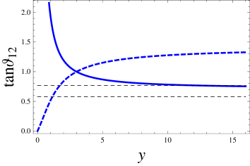
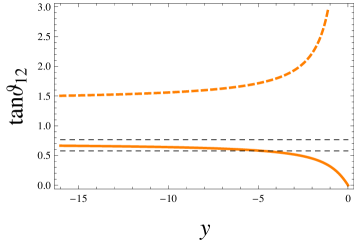
It is interesting to note that this expression is a function of y𝑦y only and independent of x𝑥x and φasubscript𝜑𝑎\varphi_{a}. The 3-σ𝜎\sigma allowed range of y𝑦y can be read from Fig. 2 and is given by

y>12.7for(y+2xcosφa+1)>0𝑦12.7for𝑦2𝑥subscript𝜑𝑎10\displaystyle y>12.7\;\;{\rm for}\;\;(y+2x\cos\varphi_{a}+1)>0
1.14<y<1.70for(y+2xcosφa+1)<01.14𝑦1.70for𝑦2𝑥subscript𝜑𝑎10\displaystyle 1.14<y<1.70\;\;{\rm for}\;\;(y+2x\cos\varphi_{a}+1)<0 (48)

for normal hierarchy and

y<4.71for(y+2xcosφa+1)<0𝑦4.71for𝑦2𝑥subscript𝜑𝑎10\displaystyle y<-4.71\;\;{\rm for}\;\;(y+2x\cos\varphi_{a}+1)<0 (49)

for inverted hierarchy. It is impossible to satisfy the data for the solar mixing angle when (y+2xcosφa+1)>0𝑦2𝑥subscript𝜑𝑎10(y+2x\cos\varphi_{a}+1)>0.

Refer to caption
Refer to caption
Figure 2: Thick solid (dashed) curve: tanθ12subscript𝜃12\tan\theta_{12} as a function of y𝑦y for y+2xcosφa+1>0(<0)𝑦2𝑥subscript𝜑𝑎1annotated0absent0y+2x\cos\varphi_{a}+1>0\;(<0). Dashed horizontal lines: 3-σ𝜎\sigma allowed range of tanθ12subscript𝜃12\tan\theta_{12}, 0.577<tanθ12<0.7660.577subscript𝜃120.7660.577<\tan\theta_{12}<0.766. The left (right) panel is for normal (inverted) hierarchy.

To consider the constraints from the mass-squared differences, we take the ratio |Δm322|/Δm212Δsuperscriptsubscript𝑚322Δsuperscriptsubscript𝑚212|\Delta m_{32}^{2}|/\Delta m_{21}^{2} because |d|2superscript𝑑2|d|^{2} is canceled in this case. Then Eqs. (43) and (44) give

ρΔmsol2Δmatm2=Δm212|Δm322|=|y+2xcosφa+1|f(y),𝜌Δsuperscriptsubscript𝑚sol2Δsuperscriptsubscript𝑚atm2Δsuperscriptsubscript𝑚212Δsuperscriptsubscript𝑚322𝑦2𝑥subscript𝜑𝑎1𝑓𝑦\displaystyle\rho\equiv\frac{\Delta m_{\rm sol}^{2}}{\Delta m_{\rm atm}^{2}}=\frac{\Delta m_{21}^{2}}{|\Delta m_{32}^{2}|}=\frac{|y+2x\cos\varphi_{a}+1|}{f(y)}, (50)

where

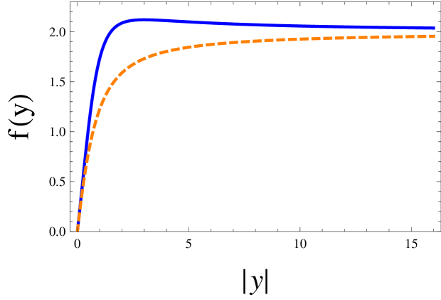
f(y)=6|y|96y+9y2.𝑓𝑦6𝑦96𝑦9superscript𝑦2\displaystyle f(y)=\frac{6|y|}{\sqrt{9-6y+9y^{2}}}. (51)

Fig. 3 shows the plots of f(y)𝑓𝑦f(y).

Refer to caption
Figure 3: Solid (Dashed) curve: f(y)𝑓𝑦f(y) for normal (inverted) hierarchy.

The experimental value of ρ=(3.19±0.19)×102𝜌plus-or-minus3.190.19superscript102\rho=(3.19\pm 0.19)\times 10^{-2} can be satisfied by tuning y+2xcosφa+10𝑦2𝑥subscript𝜑𝑎10y+2x\cos\varphi_{a}+1\approx 0.

Refer to caption
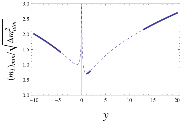
Figure 4: The mass ratio, (m1)min/Δmatm2subscriptsubscript𝑚1minΔsuperscriptsubscript𝑚atm2{(m_{1})_{\rm min}}/{\sqrt{\Delta m_{\rm atm}^{2}}}, as a function of y𝑦y when cos2φa=1superscript2subscript𝜑𝑎1\cos^{2}\varphi_{a}=1. The thick solid curves are allowed by the current experimental data.

Using the relation, 2xcosφa+y+102𝑥subscript𝜑𝑎𝑦102x\cos\varphi_{a}+y+1\approx 0, we can get

m12Δmatm216|y|((y+12cosφa)2+2(y2y+1)),similar-to-or-equalssuperscriptsubscript𝑚12Δsuperscriptsubscript𝑚atm216𝑦superscript𝑦12subscript𝜑𝑎22superscript𝑦2𝑦1\displaystyle\frac{m_{1}^{2}}{\Delta m_{\rm atm}^{2}}\simeq\frac{1}{6|y|}\left(\left(\frac{y+1}{2\cos\varphi_{a}}\right)^{2}+2(y^{2}-y+1)\right), (52)

in the leading order in ρ𝜌\rho. The minimum of m1subscript𝑚1m_{1} is obtained when cos2φa=1superscript2subscript𝜑𝑎1\cos^{2}\varphi_{a}=1 for both normal and inverted hierarchy. Fig. 4 shows (m1)min/Δmatm2subscriptsubscript𝑚1minΔsuperscriptsubscript𝑚atm2{(m_{1})_{\rm min}}/{\sqrt{\Delta m_{\rm atm}^{2}}}, that is, the m1/Δmatm2subscript𝑚1Δsuperscriptsubscript𝑚atm2{m_{1}}/{\sqrt{\Delta m_{\rm atm}^{2}}} as a function of y𝑦y when cos2φa=1superscript2subscript𝜑𝑎1\cos^{2}\varphi_{a}=1. It shows that there is a lower bound on the lightest neutrino mass, m1(3)0.03(0.05)greater-than-or-equivalent-tosubscript𝑚130.030.05m_{1(3)}\gtrsim 0.03(0.05) eV for the normal (inverted) hierarchy.

Now let us consider the bound on the effective Majorana mass for neutrinoless double-beta decay [4]. The amplitude of the neutrinoless double beta decay (0νββ0𝜈𝛽𝛽0\nu\beta\beta) is proportional to the effective Majorana mass for the 0νββ0𝜈𝛽𝛽0\nu\beta\beta defined by

|mββ||imi(UMNS)1i2|=|(Mνeff)11|=|a+2d|=d|xeiφa+2|.delimited-⟨⟩subscript𝑚𝛽𝛽subscript𝑖subscript𝑚𝑖subscriptsuperscriptsuperscriptsubscript𝑈MNS21𝑖subscriptsuperscriptsubscript𝑀𝜈eff11𝑎2𝑑𝑑𝑥superscript𝑒𝑖subscript𝜑𝑎2\displaystyle\left|\langle m_{\beta\beta}\rangle\right|\equiv\left|\sum_{i}m_{i}\left(U_{\rm MNS}^{*}\right)^{2}_{1i}\right|=\left|\left(M_{\nu}^{\rm eff}\right)_{11}\right|=\left|a+2d\right|=d\left|xe^{i\varphi_{a}}+2\right|. (53)

Similar to (52), we get

|mββ|2Δmatm216|y|((y+12cosφa)22(y1)),similar-to-or-equalssuperscriptdelimited-⟨⟩subscript𝑚𝛽𝛽2Δsuperscriptsubscript𝑚atm216𝑦superscript𝑦12subscript𝜑𝑎22𝑦1\displaystyle\frac{\left|\langle m_{\beta\beta}\rangle\right|^{2}}{\Delta m_{\rm atm}^{2}}\simeq\frac{1}{6|y|}\left(\left(\frac{y+1}{2\cos\varphi_{a}}\right)^{2}-2(y-1)\right), (54)

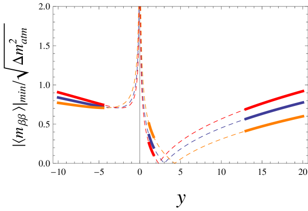
in the leading approximation in ρ𝜌\rho. The ratio |mββ|/Δmatm2delimited-⟨⟩subscript𝑚𝛽𝛽Δsuperscriptsubscript𝑚atm2{\left|\langle m_{\beta\beta}\rangle\right|}/{\sqrt{\Delta m_{\rm atm}^{2}}} has lower bounds for the allowed range in y𝑦y (thick parts in the solid blue curve in Fig. 5). Numerically we get

|mββ|/Δmatm2>0.2(for 1.13<y<1.7),>0.57(fory>13),\displaystyle{\left|\langle m_{\beta\beta}\rangle\right|}/{\sqrt{\Delta m_{\rm atm}^{2}}}>0.2\;({\rm for}\;1.13<y<1.7),\quad>0.57\;({\rm for}\;y>13),
|mββ|/Δmatm2>0.72(fory<4.5).delimited-⟨⟩subscript𝑚𝛽𝛽Δsuperscriptsubscript𝑚atm20.72for𝑦4.5\displaystyle{\left|\langle m_{\beta\beta}\rangle\right|}/{\sqrt{\Delta m_{\rm atm}^{2}}}>0.72\;({\rm for}\;y<-4.5). (55)

The model with A4subscript𝐴4A_{4} symmetry which has non-vanishing lower bound for |mββ|/Δmatm2delimited-⟨⟩subscript𝑚𝛽𝛽Δsuperscriptsubscript𝑚atm2{\left|\langle m_{\beta\beta}\rangle\right|}/{\sqrt{\Delta m_{\rm atm}^{2}}} even in the case of normal hierarchy was considered in [4]. Numerically we get similar values to theirs.
Refer to caption
Figure 5: The mass ratio, (mββ)min/Δmatm2subscriptsubscript𝑚𝛽𝛽minΔsuperscriptsubscript𝑚atm2{(m_{\beta\beta})_{\rm min}}/{\sqrt{\Delta m_{\rm atm}^{2}}}, as a function of y𝑦y when cos2φa=1superscript2subscript𝜑𝑎1\cos^{2}\varphi_{a}=1. The blue (red, orange) curve corresponds to the case b=c𝑏𝑐b=c (ξ=0.3𝜉0.3\xi=0.3, ξ=0.3𝜉0.3\xi=-0.3). The thick parts are allowed by the current experimental data.

3.2 The case bc𝑏𝑐b\not=c

As mentioned in Section 2, the case b=c𝑏𝑐b=c is not guaranteed by any symmetry. In this section we extend to the case bc𝑏𝑐b\not=c. The effective neutrino mass matrix given in (35) is now in the form:

Mνeffsuperscriptsubscript𝑀𝜈eff\displaystyle M_{\nu}^{\rm eff} =\displaystyle= U(ω)MνU(ω)=(a+2dcbcbadbadc).𝑈superscript𝜔subscript𝑀𝜈𝑈superscript𝜔𝑎2𝑑𝑐𝑏𝑐𝑏𝑎𝑑𝑏𝑎𝑑𝑐\displaystyle U(\omega)^{*}M_{\nu}U(\omega)^{\dagger}=\left(\begin{array}[]{ccc}a+2d&c&b\\ c&b&a-d\\ b&a-d&c\end{array}\right). (59)

Since b=c𝑏𝑐b=c case can already give the tribimaximal mixing matrix, we can see b𝑏b and c𝑐c cannot be so different. Therefore, we can apply the time-independent perturbation theory to diagonalize the neutrino mass matrix and expand in powers of ξ(cb)/2b𝜉𝑐𝑏2𝑏\xi\equiv(c-b)/2b. Since b𝑏b is assumed to be real, we also assume ξ𝜉\xi to be real.

Since the 1st and 2nd eigenvalues giving the Δmsol2Δsuperscriptsubscript𝑚sol2\Delta m_{\rm sol}^{2} are quasi-degenerate, the blind application of the perturbation formula gives unreasonable results. To evade this problem we diagonalized the 2×2222\times 2 sub-matrix exactly. And then we applied the perturbation formula in the basis where the first two mass-squared eigenvalues are diagonal.

The solar mass-squared difference is obtained to be

Δmsol2d2|2xcosφa+y+1+ξy|9y26y+9.similar-to-or-equalsΔsuperscriptsubscript𝑚sol2superscript𝑑22𝑥subscript𝜑𝑎𝑦1𝜉𝑦9superscript𝑦26𝑦9\displaystyle\Delta m_{\rm sol}^{2}\simeq d^{2}|2x\cos\varphi_{a}+y+1+\xi y|\sqrt{9y^{2}-6y+9}. (60)

This implies the “magic relation” corresponding to (45) is simply replaced by

2xcosφa+y+1+ξy0.2𝑥subscript𝜑𝑎𝑦1𝜉𝑦0\displaystyle 2x\cos\varphi_{a}+y+1+\xi y\approx 0. (61)

The atmospheric mass-squared difference is

Δmatm26d2|y|(1+ξ).similar-to-or-equalsΔsuperscriptsubscript𝑚atm26superscript𝑑2𝑦1𝜉\displaystyle\Delta m_{\rm atm}^{2}\simeq 6d^{2}|y|(1+\xi). (62)

Since ξ1much-less-than𝜉1\xi\ll 1, y>0(y<0)𝑦0𝑦0y>0\;(y<0) still gives normal (inverted) hierarchy.

The correction in ξ𝜉\xi to the effective mass for the 0νββ0𝜈𝛽𝛽0\nu\beta\beta, (54), is given by

|mββ|2Δmatm216|y|(1+ξ)((y+12cosφa)22(y1)+2yξy+1(2cosφa)2).similar-to-or-equalssuperscriptdelimited-⟨⟩subscript𝑚𝛽𝛽2Δsuperscriptsubscript𝑚atm216𝑦1𝜉superscript𝑦12subscript𝜑𝑎22𝑦12𝑦𝜉𝑦1superscript2subscript𝜑𝑎2\displaystyle\frac{\left|\langle m_{\beta\beta}\rangle\right|^{2}}{\Delta m_{\rm atm}^{2}}\simeq\frac{1}{6|y|(1+\xi)}\left(\left(\frac{y+1}{2\cos\varphi_{a}}\right)^{2}-2(y-1)+2y\xi{y+1\over(2\cos\varphi_{a})^{2}}\right). (63)

The minimum values in φasubscript𝜑𝑎\varphi_{a} are obtained for φa=π(0)subscript𝜑𝑎𝜋0\varphi_{a}=\pi(0) for normal (inverted) hierarchy. These are plotted in Fig. 5 as a function of y𝑦y for different values of ξ=0,±0.3𝜉0plus-or-minus0.3\xi=0,\pm 0.3. The allowed regions are drawn in thick lines. The value |ξ|0.3similar-to-or-equals𝜉0.3|\xi|\simeq 0.3 is almost maximum allowed by the 3-σ𝜎\sigma range in s13subscript𝑠13s_{13} (see Figs. 6,7). Numerically the minimum values for the normal hierarchy are given by

(|mββ|/Δmatm2)min=0.1,0.2,0.34(forξ=0.3,0,0.3,resp.).\displaystyle\left({\left|\langle m_{\beta\beta}\rangle\right|}/{\sqrt{\Delta m_{\rm atm}^{2}}}\right)_{\rm min}=0.1,0.2,0.34\;({\rm for}\;\xi=0.3,0,-0.3,\;{\rm resp.}). (64)

Since ρ0.1much-less-than𝜌0.1\rho\ll 0.1, the correction to (63) in ρ𝜌\rho does not change the results much.

For the mixing angle θ12subscript𝜃12\theta_{12} we get a formula similar to (47),

tan2θ12±22|y|y3forsign(y+2xcosφa+1+ξy)=±.similar-to-or-equals2subscript𝜃12plus-or-minus22𝑦𝑦3forsign𝑦2𝑥subscript𝜑𝑎1𝜉𝑦plus-or-minus\displaystyle\tan 2\theta_{12}\simeq\pm\frac{2\sqrt{2}|y|}{y-3}\;\;\;{\rm for}\;\;{\rm sign}(y+2x\cos\varphi_{a}+1+\xi y)=\pm. (65)

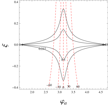
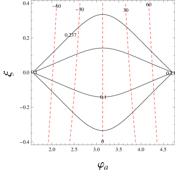
The most significant change from the case b=c𝑏𝑐b=c is that the non-vanishing θ13subscript𝜃13\theta_{13} and consequently δ𝛿\delta for non-trivial φasubscript𝜑𝑎\varphi_{a} is allowed in bc𝑏𝑐b\not=c case. The expression for s13sinθ13subscript𝑠13subscript𝜃13s_{13}\equiv\sin\theta_{13} is obtained by

s13|ξ|21+((y+1+ξy)tanφa3)2.similar-to-or-equalssubscript𝑠13𝜉21superscript𝑦1𝜉𝑦subscript𝜑𝑎32\displaystyle s_{13}\simeq\frac{|\xi|}{\sqrt{2}}\sqrt{1+\left((y+1+\xi y)\tan\varphi_{a}\over 3\right)^{2}}. (66)

The CP violating phase δ𝛿\delta is given by

δtan1((y+1+ξy)tanφa3)(modπ).similar-to-or-equals𝛿superscript1𝑦1𝜉𝑦subscript𝜑𝑎3mod𝜋\displaystyle\delta\simeq\tan^{-1}\left((y+1+\xi y)\tan\varphi_{a}\over 3\right)\;({\rm mod}\;\pi). (67)

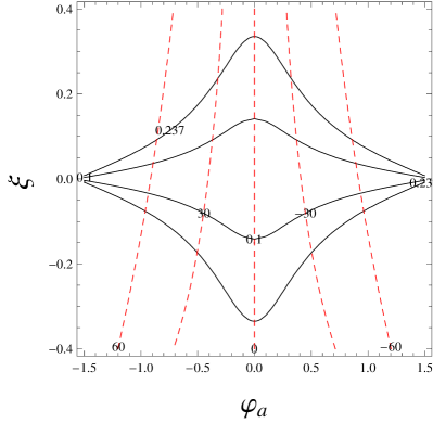
We do not have a definite prediction for s13subscript𝑠13s_{13}. But the 3-σ𝜎\sigma range in Table 1 can be accommodated. Fig. 6 (7) shows contours for the constant s13subscript𝑠13s_{13} and δ𝛿\delta for the normal (inverted) hierarchy case. We can see the 3-σ𝜎\sigma range for the s13subscript𝑠13s_{13} can be accommodated in the perturbative region for ξ𝜉\xi. All the possible values of δ𝛿\delta are allowed by the current experimental values, although relatively small values of δ𝛿\delta are preferred.

A very interesting prediction is for θ23subscript𝜃23\theta_{23}. Up to the first order in ξ𝜉\xi, the prediction for θ23subscript𝜃23\theta_{23} is still π/4𝜋4\pi/4. The first correction appears in second order in ξ𝜉\xi:

sin2θ23=0.5+𝒪(ξ2)0.5±0.01,superscript2subscript𝜃230.5𝒪superscript𝜉2plus-or-minus0.50.01\displaystyle\sin^{2}\theta_{23}=0.5+{\cal O}(\xi^{2})\approx 0.5\pm 0.01, (68)

for the 1-σ𝜎\sigma allowed ξ𝜉\xi (ξ0.1less-than-or-similar-to𝜉0.1\xi\lesssim 0.1) by s13subscript𝑠13s_{13}. Therefore if the experiments would confirm significant deviation from π/4𝜋4\pi/4 for θ23subscript𝜃23\theta_{23}, our model would be ruled out.

Refer to caption
Refer to caption
Figure 6: Solid (dashed) curves: contours for the constant s13subscript𝑠13s_{13} (δ𝛿\delta (in degrees) ) for the normal hierarchy. The inner (outer) solid lines are contours for the 3-(1-)σ𝜎\sigma values of s13subscript𝑠13s_{13}. We take y=13𝑦13y=13 (y=1.5𝑦1.5y=1.5) for the left (right) panel.
Refer to caption
Figure 7: The same with Fig. 6. But we take y=5𝑦5y=-5.

4 Conclusions

We studied a triplet Higgs model to generate Majorana neutrino masses and the mixing matrix in the framework of A4subscript𝐴4A_{4} symmetry. With the assignments of A4subscript𝐴4A_{4} representations given in Table 2, we see that

  • The tribimaximal form of the neutrino mixing matrix can be naturally obtained for b=c𝑏𝑐b=c.

  • There is a lower bound on the lightest neutrino mass: m10.03(0.05)greater-than-or-equivalent-tosubscript𝑚10.030.05m_{1}\gtrsim 0.03(0.05) eV for the normal (inverted) hierarchy.

  • There is a lower bound on the effective mass for the neutrinoless double beta decay: |mββ|/Δmatm2>0.2(0.57)delimited-⟨⟩subscript𝑚𝛽𝛽Δsuperscriptsubscript𝑚atm20.20.57{\left|\langle m_{\beta\beta}\rangle\right|}/{\sqrt{\Delta m_{\rm atm}^{2}}}>0.2(0.57) for the normal (inverted) hierarchy.

  • For bc𝑏𝑐b\not=c case, we can accommodate the data for the θ13subscript𝜃13\theta_{13}.

  • Even for bc𝑏𝑐b\not=c case, the prediction for the atmospheric mixing angle does not change much from θ23=π/4subscript𝜃23𝜋4\theta_{23}=\pi/4 and gives sin2θ230.5±0.01superscript2subscript𝜃23plus-or-minus0.50.01\sin^{2}\theta_{23}\approx 0.5\pm 0.01, which can be tested in near future.

Acknowledgments This work was supported in part by the Korea Research Foundation Grant funded partly by the Korean Government (MOEHRD) No. KRF-2007-359-C00009 and partly by Basic Science Research Program through the National Research Foundation of Korea (NRF) funded by the Ministry of Education, Science and Technology No. 20090090848 (SB) and supported partly by the Korea Research Foundation Grant funded by the Korean Government (Brain Korea 21) No.200803266004(M.C.Oh).

References

  • [1] C. Amsler et al. [Particle Data Group], Phys. Lett.  B 667, 1 (2008). M. Maltoni, T. Schwetz, M. A. Tortola and J. W. F. Valle, New J. Phys.  6, 122 (2004) [arXiv:hep-ph/0405172]; T. Schwetz, M. A. Tortola and J. W. F. Valle, New J. Phys.  10, 113011 (2008) [arXiv:0808.2016 [hep-ph]].
  • [2] P. F. Harrison, D. H. Perkins and W. G. Scott, Phys. Lett.  B 530, 167 (2002) [arXiv:hep-ph/0202074].
  • [3] K. S. Babu, E. Ma and J. W. F. Valle, Phys. Lett.  B 552, 207 (2003) [arXiv:hep-ph/0206292]; E. Ma, Mod. Phys. Lett.  A 17, 2361 (2002) [arXiv:hep-ph/0211393]; G. Altarelli and F. Feruglio, Nucl. Phys.  B 720, 64 (2005) [arXiv:hep-ph/0504165]; X. G. He, Y. Y. Keum and R. R. Volkas, JHEP 0604, 039 (2006) [arXiv:hep-ph/0601001]. M. Hirsch, A. S. Joshipura, S. Kaneko and J. W. F. Valle, Phys. Rev. Lett.  99, 151802 (2007) [arXiv:hep-ph/0703046].
  • [4] M. Hirsch, A. Villanova del Moral, J. W. F. Valle and E. Ma, Phys. Rev.  D 72, 091301 (2005) [Erratum-ibid.  D 72, 119904 (2005)] [arXiv:hep-ph/0507148].
  • [5] A. G. Akeroyd, M. Aoki and H. Sugiyama, Phys. Rev.  D 77, 075010 (2008) [arXiv:0712.4019 [hep-ph]].
  • [6] E. Ma, Phys. Rev.  D 70, 031901 (2004) [arXiv:hep-ph/0404199].
  • [7] P. H. Frampton, M. C. Oh and T. Yoshikawa, Phys. Rev.  D 66, 033007 (2002) [arXiv:hep-ph/0204273].
  • [8] J. Schechter and J. W. F. Valle, Phys. Rev.  D 22, 2227 (1980); T. P. Cheng and L. F. Li, Phys. Rev.  D 22, 2860 (1980).