The anisotropic redshift space galaxy correlation function: detection on the BAO Ring
Abstract
In a series of papers we have recently studied the clustering of LRG galaxies in the latest spectroscopic SDSS data release, which has 75000 LRG galaxies sampling 1.1 to z=0.47. Here we focus on detecting a local maxima shaped as a circular ring in the bidimensional galaxy correlation function , separated in perpendicular and line-of-sight distances. We find a significant detection of such a peak at Mpc/h. The overall shape and location of the ring is consistent with it originating from the recombination-epoch baryon acoustic oscillations (BAO). This agreement provides support for the current understanding of how large scale structure forms in the universe. We study the significance of such feature using large mock galaxy simulations to provide accurate errorbars.
1 Gravitational instability
Is the large scale structure that we see in the galaxy distribution produced by gravitational growth from some small initial fluctuations? We will explore two ways of addressing this question with measurements of the 2-point galaxy correlation:
| (1) |
where and is the local density fluctuation about the mean , and the expectation values are taken over different realizations of the model or physical process. In practice, the expectation value is over different spatial regions in our Universe, which are assumed to be a fair sample of possible realizations (see Peebles 1980). The measured redshift distance of a galaxy differs from the true radial distance by its peculiar velocity along the line-of-sight. We can split the distance into its component along the line-of-sight (LOS) and perpendicular to the LOS , where . Azimuthal symmetry implies is in general a function of and alone: .
Consider the fully non-linear fluid equations that determine the gravitational evolution of density fluctuations, , and the divergence of the velocity field, , in an expanding universe for a pressureless irrotational fluid. In Fourier space (see Eq.37-38 in bernar ):
| (2) | |||
where derivatives are over conformal time and is given by the expansion rate of the cosmological scale factor . On the left hand side and are functions of the Fourier wave vector . The integrals are over vectors and constrained to . The right hand side of the equation include the non-linear terms which are quadratic in the field and contain the mode coupling functions and . When fluctuations are small we can neglect the quadratic terms in the equations and we then obtain the linear solution . The first equation yields , which combined with the second equation yields the well known harmonic oscillator equation for the linear growth:
| (3) |
Because the Fourier transformation is linear, this equation is valid in Fourier or in configuration space. In linear theory each Fourier mode and each local fluctuation evolves independently of the others, moreover, they all grow linearly out of the initial fields with the same growth function, ie , where is the value of the field at a point (or a given Fourier mode) at some initial time and is the linear growth function, which is a solution to the above harmonic equation. In a flat universe dominated by cold dark matter (CDM) we have that and goes as the scale factor . In an accelerated phase, such as CDM, the growth halts or grows less rapidly with . Thus measurements of can be used as an independent diagnostics for accelerated expansion.
1.1 BAO signature
Consider now our observable, the 2-point function in Eq.[1]. In linear theory: . This means that on large scales, ie , where , we then expect the shape of today to be the same as the shape it took in the early universe. The prediction, ignoring redshift space distortions, is shown in Fig.1. The BAO ring corresponds to the local maxima at a radius of about . This will be tested here by comparing the linear theory prediction for the baryon acoustic oscillation (BAO) with the measurements in the large scale galaxy distribution.
t]
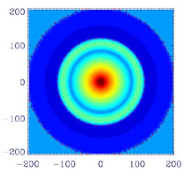

The mean BAO signature in the 2-point correlation has been detected in Luminous Red Galaxies (LRG’s) of the SDSS galaxy survey detection using the monopole, ie the average signal of in circles of constant . In paper1 ; paper4 and below we will show that the galaxy distribution has a BAO ring very similar to that predicted in the initial conditions of the CDM model.
1.2 Growth factor
On the other hand, if we knew the shape and amplitude of the initial conditions , we could then estimate from measurements of and compare it to the linear solution of Eq.[3] to test gravitational instability. But this approach is difficult in practice because there is a bias in the amplitude of galaxy clustering compare to the one in dark matter fluctuations. We could instead test gravitational growth with independence of time or initial conditions by using the linear relation between density and velocities, , where is the velocity growth factor. For a flat dark matter dominated universe and , while for a flat accelerated universe , where is the gravitational growth index and is the matter density at a redshift z where . The growth index separates out two physical effects on the growth of structure: depends on the expansion history while depends on the underlaying theory of gravity linder1 . The value corresponds to standard gravity, while is different for modified gravity, for example in the braneworld cosmology. We will show next how can be measured using redshift space distortions in the galaxy correlation function .
2 Analysis of Data
In this work we use the most recent spectroscopic SDSS data release, DR6 (dr6 ). We use the same samples and methodology here as presented in paper1 of this series. LRG’s are targeted in the photometric catalog, via cuts in the (g-r, r-i, r) color-color-magnitude cube. We need to k-correct the magnitudes in order to obtain the absolute magnitudes and eliminate the brightest and dimmest galaxies. We have seen that the previous cuts limit the intrinsic luminosity to a range , and we only eliminate from the catalog some few galaxies that lay out of the limits. Once we have eliminated these extreme galaxies, we still do not have a volume limited sample at high redshift. For the 2-point function analysis we account for this using a random catalog with identical selection function but 20 times denser (to avoid shot-noise) . The same is done in simulations.
There are about LRG galaxies with spectroscopic redshifts in the range over of the sky. We break the full sample into 3 independent subsamples with similar number of galaxies: low , middle and high . In this analysis we will just show results for the sample (see paper1 ; paper4 for other samples).
To estimate the correlation , we use the estimator of landyszalay ,
| (4) |
with a random catalog times denser than the SDSS catalog. The random catalog has the same redshift (radial) distribution as the data, but smoothed with a bin to avoid the elimination of intrinsic correlations in the data. The random catalog also has the same mask. We count the pairs in bins of separation along the line-of-sight (LOS), , and across the sky, . The LOS distance is just the difference between the radial comoving distances in the pair. The transverse distance is given by , where is the net distance between the pair. We use the small-angle approximation, as if we had the catalog at an infinite distance, which is accurate until the angle that separates the galaxy pair in the sky is larger than about 10 degrees for (see szapudiwide and matsuwide ). This condition corresponds to transverse scales larger than for our mean catalog.
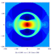
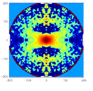
The right panel in Fig.2 shows the measurements of in the sample. As we will show below there is a remarkable agreement with the predictions (left panel) and there is good evidence for a BAO ring.

2.1 Errors and simulations
There are two sources of error or variance in the estimation of the two-point correlation: a) shot-noise which scales as one over the square root of the number of pairs in each separation bin b) sampling variance which scales with the amplitude of the correlation. It is easy to check that for the size and number density of our sample, the shot-noise term dominates over the sampling variance error. This has been confirmed in detail by using numerical simulations (see paper1 for more details). The simulation contains dark matter particles, in a cube of side (which we call MICE7680), , , , and . We have divided this big cube in cubes of side 2 x 1275Mpc/h, and taking the center of these secondary cubes as the observation point (as if we were at z=0), we apply the selection function of LRG, which arrives to z=0.47 (r=1275Mpc/h). We can obtain 8 octants from the secondary sphere included in the cube, so at the end we have 8 mock LRG catalogs from each secondary cube, which have the same density per pixel as LRG in order to have the same level of shot noise, and the area is slightly smaller (LRG occupies 1/7 of the sky with a different shape). The final number of independent mock catalogs is (27x8). We also apply redshift distortions in the line-of-sight direction , using the peculiar velocities from the simulations. The error covariance is found from the dispersion of realizations:
| (5) |
where is the measure in the k-th simulation (k=1,…M) and is the mean over M realizations (which we have checked that agrees with overall mean, indicating that volume effects are small). The case i=j gives the diagonal error (variance). In our analysis we model the errors using dark matter groups. These groups are chosen to have the same number density and amplitude of clustering as the observed LRG’s. The resulting errorbars from simulations are typically in good agreement with Jack-knife errors from the actual data (see paper1 for details). We have also checked in paper1 that we can recover the theory predictions for within the errors by using mock simulations with similar size as the real data.
2.2 Redshift space distortions
Radial displacements caused by peculiar velocities lead to redshift distortions, with two important contributions. The first, on large scale fluctuations, caused by coherent bulk motion. We see walls denser and voids bigger and emptier, with a squashing effect in the 2-point correlation function along the line-of-sight: known as the Kaiser Kaiser effect. At small scales, random velocities inside clusters and groups of galaxies produce a radial stretching pointed at the observer, known as fingers of God (FOG). Although such distortions complicate the interpretation of redshift maps as positional maps, they have the advantage of bearing unique information about the dynamics of galaxies. In particular, the amplitude of distortions on large scales yields a measure of the linear redshift distortion parameter .
In the large-scale linear regime, and in the plane-parallel approximation, the distortion caused by coherent infall velocities takes a particularly simple form. On average, large scale fluctuations in redshift space are enhanced with respect to real space because of the radial velocity infall, so that so that they are larger by a factor . This enhancement is anisotropic. In Fourier space:
| (6) |
where is the power spectrum of density fluctuations , is the cosine of the angle between and the line-of-sight, the subscript indicates redshift space, and is the velocity growth rate in linear theory.
The correlation is related to the power spectrum by a Fourier transform:
| (7) |
After integration in Eq.[7], these linear distortions in produce a distinctively anisotropic . At scales smaller than about there is a clear squashing in the correlation function caused by the peculiar velocity divergence field, this effect can be used to estimate , for example by fitting the normalized quadrupole to the data (eg see paper1 ). For the sample with z=0.15-0.30 we find , which corresponds to when we assume standard gravity ().
Redshift distortions in the linear regime produce a lower amplitude and sharper baryon acoustic peak in the LOS than in the perpendicular direction because of the coherent infall into large scale overdensities. This is illustrated in the left panel of Fig.2. A characteristic feature of this effect is a valley of negative correlations (in blue) on scales between Mpc/h, which is in very good agreement with our measurements from real SDSS data. Such a valley is absent without redshift distortions.
t]
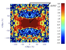
In Fig. 3, we show the signal-to-noise of in the plane for the redshift slice . This complements the signal plot in the right panel of Fig. 2. The signal-to-noise shown in Fig. 3 is for each pixel of size Mpc/h by Mpc/h (the same pixel size is used in Fig. 2). Note that there is covariance between pixels, and so this figure should be interpreted with some care (see paper1 ). Nonetheless, it demonstrates the high quality detection of a BAO ring in the plane. The triangle highlights the region , which receives not much weight in the monopole, but where the BAO ring still shows up nicely. Note that the shown is modulated by the sign of the signal: the (blue) valley of negative correlations at Mpc/h - in accord with the predictions of the Kaiser effect - are detected with significance as well. The overall coherent structure of a negative valley before a positive BAO peak (at just the right expected scales) is quite striking, and cannot be easily explained away by noise or systematic effects.
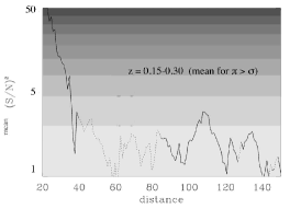
The evidence for a BAO peak in the monopole is quite convincing (see detection ; paper1 ; paper4 ). The data follows the model prediction and produces a clear detection which otherwise (without the BAO peak) is degenerate with other cosmological parameters. But the monopole signal is dominated by pairs in the perpendicular direction and here we would like to assess if the BAO peak is also significant in the radial direction. We do this by studying the signal-to-noise ratio in for . In Fig.3 this corresponds to the region inside the over-plotted triangle. We do the mean signal-to-noise inside the region as a function of the radius , in radial shells of width Mpc/h:
| (8) |
where is the sign of the signal. When the signal is negative this gives a negative contribution to the mean signal-to-noise square. If the signal is dominated by noise, positive and negative fluctuations will tend to cancel and reduced the mean . Results are shown in Fig.4. The mean signal-to-noise is always larger than unity both in the negative valley between 50-90 Mpc/h and also around the BAO peak, where the mean approaches 2. This clearly indicates that the BAO peak is also significant in the radial direction and it also has the shape that is predicted by the models, with a negative valley and a positive peak that extend in a coherent way over the expected lengths. It is unlikely that noise or systematic errors could reproduce these correlations. Similar results are found for the other redshift slices, with less significant detection for the middle slice.
t]
Acknowledgements.
We acknowledge the use of MICE simulations (www.ice.cat/mice) developed at the MareNostrum supercomputer (www.bsc.es) and with support from PIC (www.pic.es), the Spanish Ministerio de Ciencia y Tecnologia (MEC), project AYA2006-06341 with EC-FEDER funding, Consolider-Ingenio CSD2007-00060 and research project 2005SGR00728 from Generalitat de Catalunya. AC acknowledges support from the DURSI department of the Generalitat de Catalunya and the European Social Fund.References
- (1) F. Bernardeau, S. Colombi, E. Gaztañaga, and R. Scoccimarro, PhysRev 367, 1 (2002), arXiv:astro-ph/0112551.
- (2) D. J. Eisenstein, I. Zehavi, D. W. Hogg, R. Scoccimarro, M. R. Blanton, R. C. Nichol, R. Scranton, H.-J. Seo, M. Tegmark, Z. Zheng, et al., ApJ 633, 560 (2005), arXiv:astro-ph/0501171.
- (3) A. Cabré and E. Gaztañaga, ArXiv e-prints 2460 (2008), 0807.2460.
- (4) E. Gaztanaga, A. Cabre, and L. Hui, ArXiv e-prints 807 (2008), 0807.3551.
- (5) E. V. Linder, PRD 72, 043529 (2005), arXiv:astro-ph/0507263.
- (6) N. Kaiser, MNRAS 227, 1 (1987).
- (7) J. K. Adelman-McCarthy, M. A. Agüeros, S. S. Allam, C. Allende Prieto, K. S. J. Anderson, S. F. Anderson, J. Annis, N. A. Bahcall, C. A. L. Bailer-Jones, I. K. Baldry, et al., ApJS 175, 297 (2008), %****␣ref.bbl␣Line␣75␣****arXiv:0707.3413.
- (8) S. D. Landy and A. S. Szalay, ApJ 412, 64 (1993).
- (9) I. Szapudi, ApJ 614, 51 (2004), arXiv:astro-ph/0404477.
- (10) T. Matsubara, ApJ 535, 1 (2000), arXiv:astro-ph/9908056.