Protein Interaction Networks - More than Mere Modules

Author Summary (193 words):

Cellular function is widely believed to be organized in a modular fashion. On all scales and at all levels of complexity, relatively independent sub-units perform relatively independent sub-tasks of biological function. This functional modularity must be reflected in the topology of molecular networks. But how a functional module should be represented in an interaction network is an open question. In protein-interaction networks (PIN), one can identify a protein-complex as a module on a small scale, i.e. modules are understood as densely linked, resp. interacting, groups of proteins, that are only sparsely interacting with the rest of the network.

In this contribution, we show that extrapolating this concept of cohesively linked clusters of proteins as modules to the scale of the entire PIN inevitable misses important and functionally relevant structure inherent in the network. As an alternative, we introduce a novel way of decomposing a network into functional roles and show that this represents network structure and function more efficiently. This finding should have a profound impact on all module assisted methods of protein function prediction and should shed new light on how functional modules can be represented in molecular interaction networks in general.

Abstract (302 words):

It is widely believed that the modular organization of cellular function is reflected in a modular structure of molecular networks. A common view is that a “module” in a network is a cohesively linked group of nodes, densely connected internally and sparsely interacting with the rest of the network. Many algorithms try to identify functional modules in protein-interaction networks (PIN) by searching for such cohesive groups of proteins.

Here, we present an alternative approach independent of any prior definition of what actually constitutes a “module”. In a self-consitent manner, proteins are grouped into “functional roles”, if they interact in similar ways with other proteins according to their functional roles. Such grouping may well result in cohesive modules again, but only if the network structure actually supports this.

We applied our method to the PIN from the Human Protein Reference Database and found that a representation of the network in terms of cohesive modules, at least on a global scale, does not optimally represent the network’s structure because it focusses on finding independent groups of proteins. In contrast, a decomposition into functional roles is able to depict the structure much better as it also takes into account the interdependencies between roles and even allows groupings based on the absence of interactions between proteins in the same functional role, as is the case for transmembrane proteins, which could never be recognized as a cohesive group of nodes in a PIN.

When mapping experimental methods onto the groups, we identified profound differences in the coverage suggesting that our method is able to capture experimental bias in the data, too. For example yeast-two-hybrid data were highly overrepresented in one particular group.

Thus, there is more structure in protein-interaction networks than cohesive modules alone and we believe this finding can significantly improve automated function prediction algorithms in the future

Abbreviations: PPI, protein protein interaction; GO, Gene Ontology; HPRD, Human Protein Reference Database

1 Introduction

Biological function is believed to be organized in a modular and hierarchical fashion [1]. Genes make proteins, proteins from cells, cells form organs, organs form organisms, organisms form populations and populations form ecosystems. While the higher levels of this hierarchy are well understood, and the genetic code has been deciphered, the unraveling of the inner workings of the proteome poses one of the greatest challenges in the post-genomic era [2]. The development of high-throughput experimental techniques for the delineation of protein-protein interactions as well as modern data warehousing technologies to make data available and searchable are key steps towards understanding the architecture and eventually function of the cellular network. These data now allow for searching for functional modules within these networks by computational approaches and for assigning of putative protein functions based on such data.

A recent review by Sharan et al. [2] surveys the current methods of network based prediction methods for protein function. Proteins must interact to function. Hence, we can expect protein function to be encoded in a protein interaction network. The basic underlying assumption of all methods of automated functional annotation is that pairwise interaction is a strong indication for common function.

Sharan et al. differentiate two basic approaches of network based function prediction: “direct methods”, which can be seen as local methods applying a “guilt-by-association” principle [3] to immediate or second neighbors in the network, and “module assisted” methods which first cluster the network into modules according to some definition and then annotate proteins inside a module based on known annotations of other proteins in the module. So instead of “guilt-by-association”, one could speak of “kin-liability”. The latter approach to function prediction necessarily needs a concept of what is to be considered a module in a network. Most researchers consider cohesive sets of proteins which are highly connected internally, but only sparsely with the rest of the network [4, 5, 6, 7, 8, 9, 10, 11, 12, 13, 14]. Such methods have yielded considerable success at the level of very small scale modules and in particular protein complexes.

Does the concept of a module as a group of cohesively interacting proteins also extend to larger scales? Some researchers have argued that modularity in this sense is a universal principle such that small cohesive modules combine to form larger cohesive entities in a nested hierarchy [15, 16]. But is this view really adequate to describe the architecture of protein interactions? Recently, Wang and Zhang [17] even questioned whether cohesive clusters in protein interaction networks do carry biological information at all and suggested a simple network growth model based on gene duplication which would produce the observed structural cohesiveness as “an evolutionary byproduct without biological significance”. We will not go as far as questioning the content of biological information in the network structure but rather argue against the model of a cohesively linked group of nodes in a network as an adequate proxy for a functional module on all scales of the network.

Consider as first example protein complexes. Indeed, they consist of proteins working together and experimentally isolated together. Only the large scale analysis of protein complexes [18, 19] revealed that they are more dynamic than previously assumed. Many proteins can be found not only in a single, but in a multitude of complexes. The information of proteins connecting complexes will be lost when searching only for cohesively interacting groups of proteins. As a second example, consider transmembrane proteins, like receptors in signal transduction cascades. They tend to interact with many different cytoplasmic proteins as well as with their extracellular ligands. Still, only rarely do different transmembrane receptors interact with each other. Thus, the functional class of transmembrane receptors will not be identified when looking for cohesive modules.

Here, we asked whether these features, which are not covered by algorithms searching for cohesive modules, are also present in the overall structure of the cellular network. If this would be the case, methods searching only for cohesive modules would not be able to identify them. We group proteins self-consistently into functional roles if they interact in similar ways with other proteins according to their functional roles. Such a role may well be a cohesive module, meaning that proteins in this class predominantly interact with other proteins of this class, but it does not have to. In other words, we do not impose a structure of cohesive modules on the network in our analysis but rather find the structural representation that is best supported by the data. Using the abstraction of a functional role, we generated an ’image graph’ of the original network which depicts only the predominant interactions among classes of proteins and thus allowing a bird’s eye view of the network.

In the case of protein interaction network studied here, we found sound evidence that cohesive modules on a global scale do not adequately represent the network’s global structure. We found groups of proteins acting as intermediates and specifically connecting other groups of proteins. Furthermore, we even identified a group of proteins which was only sparsely connected within itself, but with similar patterns of interaction to other proteins. Thus, approaches searching only for cohesive modules might not be sufficient to represent all characteristics of cellular networks. Furthermore, our findings suggest that hierarchical modularity as nested, cohesively interacting groups of proteins has to be reconsidered as a universal organizing principle.

2 Functional Role Decomposition and Image Graphs

In which cases does a clustering of a network into cohesive modules not reflect its original architecture? Consider the toy network in Figure 1 a). There are four known types of proteins in this network. Type $A$ may represents some biological process involving five proteins connected to four proteins of type $B$. These are linked to another biological process $C$ which involves five further proteins which finally are linked to four proteins of type $D$. Not all nodes of the same type necessarily share the same set of neighbours. Some nodes of the same type do not have any neighbours in common with nodes of their type or have more neighbours in common with nodes of a different type. This shows that in this hypothetical example, direct methods of functional annotations may be limited in their accuracy.

Figure 1: An example network and possible image graphs. a) A simple example network of nodes of 4 different types identified by their structural position. Nodes of types A and C are densely connected among themselves. The nodes of type B have connections to both nodes of types A und B, but not among themselves, i.e. they mediate between types A and C. The nodes of type D only have connections to nodes of type C, but not among each other, i.e. they form a periphery to type C nodes. (b) and c) Two possible image graphs for the functional understanding of this network show the connections among groups of nodes. A typical network clustering will aggregate nodes into clusters densely connected internally but only sparsely connected to the rest, as depicted in the left image graph. This will result in grouping nodes of types A and B together and nodes of type C+D together. Because of aggregating nodes into cohesive groups any such algorithm will never recognize nodes of type C and D as different and hence miss essential part of the network s structure. On the opposite, the right image graph correctly captures the network structure of the 4 different types as the 4 different nodes in the image graph. d) and e) The adjacency matrices of our example network with rows and columns ordered according to the two decompositions shown above. A black square in position $(i,j)$ indicates the existence of a link connecting node $i$ with node $j$. Rows and columns are ordered such that nodes in the same group are adjacent. The internal order of the nodes in the groups is random. Each block in the matrix corresponds to a possible edge in the image graph. The left matrix shows the adjacency matrix for the output of a typical clustering algorithm which groups nodes of type A and B, as well as C and D together. Clearly we see dense blocks along the diagonal and sparse blocks on the off-diagonal of the matrix as expected. The right matrix depicts the adjacency matrix with rows and columns according to the actual types of the nodes. All empty blocks in this matrix correspond to a missing edge in the image graph and all populated blocks are represented by an edge in the image graph. We see that for this network, the image graph perfectly captures the structure of the network.

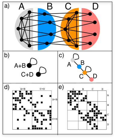
Clustering the network into cohesive modules cannot capture the full structure of the network. The nodes of type B will never be recognized as a proper cluster, because they are not connected internally at all. An attempt to identify such groups was made by Guimera et al. who quantified the error to such a cohesive clustering approach in a “participation coefficient” which is then used to differentiate groups of proteins by this participation coefficient. [20].

The structure of the example network can, however, be perfectly captured by a simple image graph with 4 nodes (Fig. 1 c). The nodes in an image graph correspond to the types of nodes in the network. Nodes of type $A$ are connected to other nodes of type $A$ and to nodes of type $B$. Nodes of type $B$ have connections to nodes of types $A$ and $C$ and so forth. The concept of defining types of nodes by their relation to other types of nodes is known as “regular equivalence” in the social sciences [21, 22]. Structure recognition in networks can then be seen as finding the best fitting image graph for a network. In this context, clustering into functional modules means representing the network by an image graph consisting of isolated, self-linking nodes. Once an assignment of nodes into classes is obtained, the rows and columns of the incidence matrix can be reordered such that rows and columns corresponding to nodes in the same class are adjacent (Fig. 1 d and e). Since the rows and columns are not ordered within a certain class, this leads to a characteristic structure with dense blocks in the adjacency matrix corresponding to the links in the image graph and sparse or zero blocks corresponding to the links absent in the image graph. Structure recognition in networks is therefore also called “block modelling” and together with the concepts of structural and regular equivalence has a long history in the social sciences [23, 24]. In our further discussion, we will denote image graphs that consist only of isolated, self-linked nodes as in Figure 1 b), “diagonal image graphs” due to the block structure along the diagonal in the adjacency matrix that they induce. Accordingly, we will call all other image graphs “non-diagonal image graphs”.

2.1 Calculation

But how do we find the best fitting image graph? The problem amounts essentially to aligning a small graph with $q$ nodes to a large network with $N$ nodes. This involves finding an image graph and a mapping $\tau$ of the $N$ nodes of the network to the $q$ types of nodes such that the mismatch between network and image graph is minimal. Suppose we were given the $q\times q$ adjacency matrix $B_{rs}$ of our image graph together with the $N\times N$ adjacency matrix $A_{ij}$ of our network . Let $\tau$ be the mapping of the $N$ nodes to the $q$ different types, such that $\tau_{i}\in\{1,..,q\}$ for all $i\in\{1,..,N\}$. To optimize the mapping $\tau$ we minimize the following error function:

$$E(\tau,B) = \frac{1}{M}\sum_{i\neq j}^{N}(A_{ij}-B_{\tau_{i}\tau_{j}})(w_{ij}-p_{ij})$$ (1)

$$= \underbrace{\frac{1}{M}\sum_{i\neq j}^{N}(w_{ij}-p_{ij})A_{ij}}_{\mathcal{Q}_{\mbox{\tiny max}}<1}-\underbrace{\frac{1}{M}\sum_{i\neq j}^{N}(w_{ij}-p_{ij})B_{\tau_{i}\tau_{j}}}_{\mathcal{Q}(\tau,B)\leq\mathcal{Q}_{\mbox{\tiny max}}}.$$ (2)

in which $A_{ij}$ is the $\{0,1\}$ adjacency matrix of the network under study. $w_{ij}$ denotes the weight given to an edge between nodes $i$ and $j$. If an edge is absent in the network, $w_{ij}$ is naturally zero. As before $B_{\tau_{i}\tau_{j}}$ is the image graph and $p_{ij}$ is a penalty term discussed below. The normalization constant $M=\sum_{i\neq j}w_{ij}$ is used to bound the error by one. This error function gives a weight proportional to $(w_{ij}-p_{ij})$ to errors made on fitting the edges in the network and a weight of $p_{ij}$ to errors made on fitting the absent edges in the network. The penalty term $p_{ij}$ is chosen such that the total error weight on all edges in the network is equal to the total error weight on all absent edges in the network:

$$\sum_{i\neq j}^{N}A_{ij}(w_{ij}-p_{ij})=\sum_{i\neq j}^{N}(1-A_{ij})p_{ij}.$$ (3)

This can be easily achieved by setting $p_{ij}=(\sum_{k\neq i}w_{ik}\sum_{l\neq j}w_{lj})/\sum_{k\neq l}w_{kl}$. The first term of equation (2) neither depends on the mapping of nodes to types $\tau$ nor on the image graph $B_{rs}$. It can be interpreted as the maximum value of a quality function $\mathcal{Q}$ measuring the fit of the image graph to the network which would be obtained for a perfect fit, i.e. $B_{\tau_{i}\tau_{j}}=A_{ij}$ for all $(i,j)$. The second term then corresponds to the quality of the actual fit for the given image graph and mapping. The error is simply the difference between the best and any sub-optimal fit and minimizing $E$ and maximizing $\mathcal{Q}$ are equivalent.

If we assume a diagonal image graph $B_{rs}=\delta_{rs}$ we recover in $\mathcal{Q}$ of equation (2) a popular quality function for graph clustering known as Newman modularity [25, 20, 17]. We can hence directly compare the fit of different given image graphs to one network by the maximum score $\mathcal{Q}$ than can be obtained by optimizing the mapping $\tau$ of nodes in the network to the classes represented as nodes in that image graph. The overall optimal image graph with a given number of nodes $q$ and the optimal assignment $\tau$ into the $q$ classes can be found directly by searching for the assignment $\tau$ which maximizes [26, 27]

$$\mathcal{Q}^{*}(\tau)=\frac{1}{2M}\sum_{r,s}^{q}||\sum_{i\neq j}^{N}(w_{ij}-p_{ij})\delta_{\tau_{i}r}\delta_{\tau_{j}s}||.$$ (4)

The image graph which allows the highest value of $\mathcal{Q}$ among all possible image graphs with this number of classes can be read off from the assignment $\tau$ that maximizes (4). It must be such that $B_{rs}=1$, if the argument in the absolute value in (4) is strictly positive, and zero otherwise. One can view $B_{rs}$ as a lossy compression of the original network, in contrast to recently introduced lossless network compression methods for biological analysis [28]. Since most of the currently available data on protein interaction is noisy and incomplete, we find a lossy compression most adequate for the analysis of the large scale structure of the network.

3 Results

3.1 Network analysis

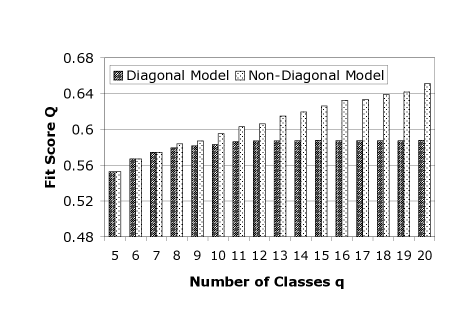
Using the quality function introduced above, we analysed the HPRD protein interaction network containing 8,500 nodes. We considered the entire network and optimised $\mathcal{Q}^{*}$ from (4) - thus finding optimal image graphs and assignments of nodes into classes. As expected, with increasing number of classes $q$, the fit between the actual network and the image graphs becomes better (Fig. 2, left panel). Restricting the image graphs to a diagonal form $B_{rs}=\delta_{rs}$ also limited the fit score. The maximum fit score was equal to $\mathcal{Q}_{\mbox{\tiny max}}=0.98$. Therefore, even with a very small number of classes, already $2/3$ of the link structure in the network was captured. The maximum of $\mathcal{Q}$ for a diagonal image graph was reached at $q=11$ and further addition of classes did not increase this value any more. For $q<8$ the fit scores for diagonal and non-diagonal image graphs were equal because for less than 8 classes the best image graphs were in fact diagonal. Only beyond this point, the additional degrees of freedom of the non-diagonal image graphs allowed better fit scores.

Figure 2: Fit scores and generalization error. Left: Comparison of highest fit scores $Q$ and $\mathcal{Q}^{*}$ for the full dataset with 32,331 interactions. Clustering methods aggregating nodes into cohesive groups (diagonal image graphs) cannot improve the score beyond a certain limit, while non-diagonal image graphs are able to capture more and more structure as the image graph gets larger and larger. Right: After removing 1000 links from the data as test-set, we optimized the assignment of nodes into classes according to (2) using only the remaining links and keeping the image graphs fixed to those found in the runs that lead to the figure on the left. With the assignment of nodes into classes for this training set of links, we computed the score on the test set of links. The figure shows average and standard deviation over 100 repetitions of this experiment.

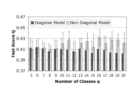
The question now is, whether these additional degrees of freedom in the image graph actually convey information or only led to overfitting. We therefore divided the $32,331$ links of the network into a test- and a training-set of $1,000$ and $31,331$ links, respectively. Using the optimal image graphs obtained on the full data set and diagonal image graphs for comparison, we optimized $\mathcal{Q}$ from (2) on the training-set of links and with the resulting mapping of nodes into classes calculated the fit score $\mathcal{Q}$ on the test-set. The fit score on the training-set of links (data not shown) was close to the full data set. We fixed the non-diagonal image graphs because the comparison is made to diagonal image graphs which were unaltered, too.

Both, diagonal and non-diagonal image graphs, showed overfitting to some extent. The score on the test set is lower than on the training set (Fig.2, right panel). However, for more than 8 classes, the non-diagonal image graphs not only allowed a better fit as discussed, but also scored better on the test-set, i.e. the increased fit value also generalized! The non-diagonal image graphs do contain more information about the network than the diagonal image graphs.

It has to be considered that using a test-set containing $3.2\%$ of all links was a drastic disturbance of the system. If we assigned nodes into $q=8$ equal sized classes, we expect approximately $2/(q(q+1))\approx 3\%$ of all links in one block. So above this point, the test set we removed was more than the typical number of links in a block. Also, consider the average degree of $\langle k\rangle\approx 8$ interactions per protein in the network. Removing a single link means removing on average $1/8$ of the neighbourhood of the nodes connected by this edge. For the 1,000 edges in the test-set, this could have happened to 2,000 nodes and thus to almost one quarter of all nodes. This explains the large fluctuations and may also explain that for $q=12$ the non-diagonal image graph cannot outperform the diagonal one.

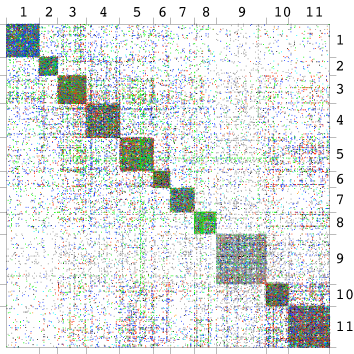
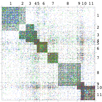
Figure 3 shows two representations of the adjacency matrix of the PIN. On the left hand side, rows and columns are ordered according to the assignment of nodes in classes when fitting a diagonal image graph, i.e. when searching for cohesive modules. On the right hand side, the rows and columns are ordered according to the assignment of nodes into classes with the highest scoring non-diagonal image graphs. In both cases we allowed for 11 classes. We have chosen this number of classes because the diagonal models did not achieve larger scores when allowing more classes. The non-diagonal image graphs led to a different assignment of nodes into classes with higher score but further increase of the number of classes did not lead to significant improvement in the generalization error (Fig. 2, right panel). Note the similarities and differences in the matrix when ordered after fitting a diagonal image graph and after fitting a non-diagonal image graph.

The non-diagonal models also allowed capturing groups of proteins that mediate between cohesive clusters such as group $2$ or that form a cohesive overlap between cohesive clusters, such as groups $4$ and $5$ or $9$ and $10$.

Figure 3: Comparison of block assignment. For $11$ classes, we show the adjacency matrix of the HPRD protein interaction network with rows and column ordered to show diagonal and non-diagnal block structure plus the corresponding image graphs for diagonal block models and non-diagonal block models. Note how the non-diagonal models allow to capture overlap between cohesive blocks but also to detect groups of nodes which are non-cohesive but have similar connection patterns to other classes of proteins. The color of the links codes the experiment type: Y2H: grey, in-vitro: blue, in-vitro+Y2H: turquoise, in-vivo: green, in-vivo+Y2H:orange, in-vivo+in-vitro: red, in-vivo+in-vitro+Y2H:black.

3.2 Biological interpretation

When comparing the cohesive module to the functional role model (Fig. 3) the most distinguishing feature was the existence of connections between sets of proteins in the latter. Groups of proteins existed, which all performed the same “functional role” of connecting two other groups of proteins. Thus, a separation of the cellular network into cohesive modules omits distinct characteristics of the network. In the functional role model, groups were connected to other groups by a distinct set of additional proteins. These ’connector groups’ may well be themselves cohesive, but do not have to. This was illustrated by class 2, where most of the proteins are not interacting with other proteins in the class, but with those of groups 1 and 3.

To evaluate the biological significance of this result, we performed a Gene Ontology enrichment analysis for all clusters. Class 2 was significantly ($E<10^{-27}$) enriched in proteins annotated as belonging to the membrane and plasma membrane compartment. Indeed, this class contained many transmembrane proteins like for example Cadherin. These proteins typically do not interact with many other transmembrane proteins, but with their extracellular binding partners and, in the case of transmembrane receptors, with cytoplasmic signal transmitters. Indeed we found that group 1, highly interacting with proteins of class 2, mainly consisted of proteins localised in the extracellular region ($E=2.54E^{-168}$). Furthermore, group 3 also strongly interacting with proteins of class 2, was enriched in proteins associated with the plasma membrane ($E=2.84E^{-28}$) and involved in signal transduction ($E=2.72E^{-20}$). Thus, the transmembrane proteins of class 2 are the perfect biological implementation of proteins not interacting with each other, but with proteins of defined other classes (nodes of type B in figure 1 a). A complete GO annotation of all clusters of classifications into $q=5$ to $q=11$ classes is given in our supporting material at http://domains.bioapps.biozentrum.uni-wuerzburg.de/ppi.

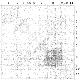
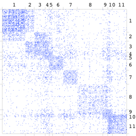
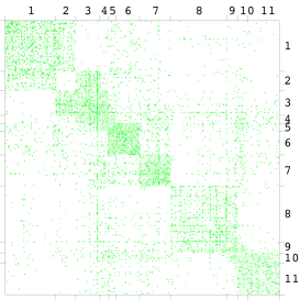
In the previous analyses, we considered all data from HPRD, as they are manually curated and therefore of a high quality. To unravel a possible bias btween different experimental methods, we plotted the data for three different experimental approaches separately. The ordering of rows and columns, i.e. the assignment of proteins into functional roles, was kept from figure 3. Instead of plotting all types of interactions on top of each other, the adjacency matrices for interactions which are backed by in-vivo, in-vitro and yeast-two-hybrid [29] (Y2H) experiments were shown separatly (Fig. 4). The in-vitro and in-vivo data nicely resembled the overall picture while the Y2H data did not follow this pattern. To test how well the overall model described the three experimental methods, we calculated the fit function $\mathcal{Q}$ for each. Here, the assignment of nodes into functional roles was taken from figure 3. The fit score for the interactions backed only by Y2H experiments was much lower than the scores of any of the other experimental methods. Thus the Y2H interactions cannot depict the full range of possible protein-protein interactions. Rather, the data based on yeast two hybrid showed a prevalence for class number 8 in figure 4. In this cluster nuclear proteins were significantly over-represented ($8.42E^{-10}$). In the Y2H [30] assay, the tested proteins are fused to parts of a transcription factor. Their interaction is measured by the transcription of a reporter gene. Therefore, the proteins have to be within the nucleus. Thus, a bias towards interactions of proteins which naturally reside in the nucleus can be expected in Y2H data.

Figure 4: Comparison of block assignment. The same assignment of nodes into classes as used in Figure 3 for but 3 different types of interactions separately. Left: Interactions reported only for yeast-2-hybrid experiments (gray). Middle: Interactions reported only in in-vitro experiments (blue). Right: Interactions reported only in in-vivo experiments (green). While in-vitro and in-vivo data is highly correlated, the interactions found in Y2H experiments are enriched in class 8.

Table 1: Fitscore for different types of interactions. Given the assignment of nodes into $q=11$ classes and the image graphs from figure 3, we calculated the fit score $Q$ for each type of interaction seperately with equation (2). Compare to figure 4 which singles out those links which are only supported by Y2H, or only in-vivo or only in-vitro experiments.

Experiment type	Diagonal Image Graph	Non-Diagonal Image Graph
yeast 2-hybrid	0.28	0.30
in vitro	0.53	0.56
in vitro + yeast 2-hybrid	0.51	0.55
in vivo	0.60	0.60
in vivo + yeast 2-hybrid	0.59	0.62
in vivo + in vitro	0.59	0.61
in vivo + in vitro + yeast 2-hybrid	0.64	0.64

4 Discussion

Using a suited algorithm, any network can be separated into cohesive groups of nodes with more internal than external connections. Accordingly, also protein-protein interaction networks can be divided into comparably independent units as putative functional modules [4]. Do these modules really reflect a typical characteristic of the cellular network? Here, we used an alternative approach for the clustering of protein interactions. We grouped proteins of a similar functional role together. The functional role was defined by the interactions with proteins of other groups. In contrast to cohesive modules, which are more or less independent, groups which specifically linked other groups of proteins could be identified. Thus, an interconnectivity of biological units as in the case of shared components in protein complexes can also be observed at the cellular level. Using a Gene Ontology based classification of all proteins within the modules, we found that these roles are mainly determined by cellular localisation but also function. Although possibly not too surprising to the biologist, this result underlines that the classes we identified by automatic clustering do represent a biological signal.

Using HPRD as data source, a large-scale set of interactions with, on average, eight connections per protein could be analysed. As HPRD contains manually curated data, their quality should be high enough to extend the results to higher coverage. The analysis of interactions derived by different experimental methods revealed a bias in the coverage especially for yeast-two-hybrid data. The great difference of the protein interactions verified only by Y2H to the other methods reminds us to pay attention to the careful weighting of quality and quantity. As large scale binary interaction analysis were mainly based on Y2H, using high coverage data like the one from yeast or Drosophila melanogaster might even blur the signal. Another drawback was the small amount of interactions per protein, which is around three to four for the yeast, fly and nematode sets analysed in the study by Wang and Zhang [17]. Still, it would be interesting to compare networks between different organisms to see whether there are changes in the clusters correlated for example with the emergence of multicellularity. But, reliable results can only be obtained when analysing data sets of comparable quality and size [31].

In summary our analysis showed that protein interaction networks are more than sparsely interacting cohesive modules. Rather, groups of proteins are connected by distinct sets of other proteins. These may be highly connected to each other, but do not have to be. Therefore, functional roles and corresponding image graphs might be better descriptors for the characteristics of a protein interaction network than cohesive modules alone. They may help to further improve protein function prediction based on protein-interaction networks.

5 Materials and Methods

5.1 PPI network.

We used the binary PPI data from the HPRD [32] (Version 6). HPRD protein identifiers and experiment types used to support their connection were extracted. The experiment types were transformed to weights according to table 2. The analysis was restricted to the largest connected component containing 32,331(out of 34,367) interactions of 8,756 proteins (out of 8,919). These interactions do not include data inferred from protein complexes which may introduce errors and bias into the network structure [17].

Table 2: Experiment type to link weight transformation. We valued the different experiments compiled in the HPRD database differently, giving lowest weight to interactions found in yeast-2-hybrid experiments only and highest to those interactions found in vivo, in vitro and Y2H experiments. These weights are only to represent a ranking of a practitioners belief in their validity.

Experiment type	Weight	# of interactions	distinct proteins involved
yeast 2-hybrid	1	6,580	3,727
in vitro	2	7,872	4,302
in vitro+yeast 2-hybrid	3	1,298	1,523
in vivo	4	6,721	3,826
in vivo+yeast 2-hybrid	5	824	1,119
in vitro+in vivo	6	6,877	3,781
in vitro+in vivo+yeast 2-hybrid	7	2,159	2,201

5.2 Clustering.

We optimized (4) and (2) using Simulated Annealing [33]. Details about the implementation can be found in [26] and [34], respectively. To obtain the left panel of figure 2, for $q=5$ to $q=20$ classes, we chose the best of 10 runs, each, for both the fit of a diagonal block model as well as the detection of a non-diagonal block model. The cooling factor for sets with more than ten classes was changed from 0.99 to 0.999 to decrease the false positive rate of local optima. To obtain the right panel of figure 2 we randomly divided the original set of links into a test-set of 1000 links and the remaining set was used as a training-set. We used the image graphs, both diagonal and non-diagonal, found in the earlier experiment to optimize the fit score on the training-set. The data shown are the fit scores of the test set, averaged over ten different partitions of the links into training- and test-set.

5.3 GO Term enrichment analysis.

The HPRD identifiers and their corresponding GO identifiers were taken from the same HPRD dataset as the PPI network, re-formatted and saved into a file readable by the Ontologizer [35]. For the Ontologizer the file gene_ontology.obo created by the GO project [36] was be downloaded.

References

- [1] Barabási AL, Oltvai Z (2004) Network biology: Understanding the cells’s functional organization. Nature Reviews Genetics 5:101–113.
- [2] Sharan R, Ulitsky I, Shamir R (2007) Network-based prediction of protein function. Molecular Systems Biology 3:88.
- [3] Oliver S (2000) Guilt-by-association goes global. Nature 403:601–603.
- [4] Spirin V, Mirny L (2003) Protein complexes and functional modules in molecular networks. Proc Natl Acad Sci USA 100:12123–12128.
- [5] Cui G, Chen Y, Huang D, Han K (2008) An algorithm for finding functional modules and protein complexes in protein-protein interaction networks. J Biomed Biotechnol 2008:860270.
- [6] Hwang W, Cho Y, Zhang A, Ramanathan M (2006) A novel functional module detection algorithm for protein-protein interaction networks. Algorithms Mol Biol 1:24.
- [7] Palla G, Derenyi I, Farkas I, Vicsek T (2005) Uncovering the overlapping community structure of complex networks in nature and society. Nature 435:814.
- [8] Adamcsek B, Palla G, Farkas IJ, Derényi I, Vicsek T (2006) Cfinder: locating cliques and overlapping modules in biological networks. Bioinformatics 22:1021–1023.
- [9] Bu D, Zhao Z, Cai L, Xue H, Lu H, et al. (2003) Topological structure analysis of the protein-protein interaction network in budding yeast. Nucleic Acids Res 31:2443–2450.
- [10] Dunn R, Dudbridge F, Sanderson CM (2005) The use of edge-betweenness clustering to investigate biological function in protein interaction networks. BMC Bioinformatics 6:39.
- [11] King AD, Przulj N, Jurisica I (2004) Protein complex prediction via cost-based clustering. Bioinformatics 20:3013–3012.
- [12] Krognan NJ, Cagney G, Yu H, Zhong G, Guo X, et al. (2006) Global landscape of protein complexes in yeast saccharomyces cerevisiae. Nature 440:637–643.
- [13] Pereira-Leal JB, Enright AJ, Ouzounis CA (2004) Detection of functional modules from protein interaction networks. Proteins 54:49–57.
- [14] Przulj N, Wiggle DA, Jurisica I (2004) Functional topology in a network of protein interactions. Bioinformatics 20:340–348.
- [15] Ravasz E, Somera A, Mongru DA, Oltvai ZN, Barabási AL (2002) Hierarchical organization of modularity in metabolic networks. Science 297:1551.
- [16] Clauset A, Moor C, Newman M (2008453) Hierarchical structure and the prediction of missing links in networks. Nature :98–101.
- [17] Wang Z, Zhang J (2007) In search of the biological significance of modular structures in protein networks. PLoS Comput Biol 3:e107.
- [18] Gavin A, Aloy P, Grandi P, Krause R, Boesche M, et al. (2006) Proteome survey reveals modularity of the yeast cell machinery. Nature 440:631–636.
- [19] Gavin A, Bösche M, Krause R, Grandi P, Marzioch M, et al. (2002) Functional organization of the yeast proteome by systematic analysis of protein complexes. Nature 415:141–147.
- [20] Guimerà R, Nunes Amaral L (2005) Functional cartography of complex metabolic networks. Nature 433:895–900.
- [21] White D, Reitz K (1983) Graph and semigroup homomorphisms. Soc Networks 5:193–234.
- [22] Lorrain F, White H (1971) Structural equivalence of individuals in social networks. J Math Sociol 1:49–80.
- [23] Doreian P, Batagelj V, Ferligoj A (2005) Generalized Blockmodeling. New York, NY, USA: Cambridge University Press.
- [24] Wasserman S, Faust K (1994) Social Network Analysis. Cambridge University Press.
- [25] Newman MEJ, Girvan M (2004) Finding and evaluating community structure in networks. Phys Rev E 69:026113.
- [26] Reichardt J, White DR (2007) Role models for complex networks. Eur Phys J B 60:217–224.
- [27] Reichardt J (2008) Structure in Networks, volume 766 of Lecture Notes in Physics. Springer-Verlag Berlin Heidelberg.
- [28] Royer L, Reimann M, Andreopoulos B, Schroeder M (2008) Unraveleing protein networks with power graph analysis. PLoS Comput Biol 4:e1000108.
- [29] Fields S, Song O (1989) A novel genetic system to detect protein-protein interactions. Nature 340:245–246.
- [30] Ito T, Chiba T, Ozawa R, Yoshida M, Hattori M, et al. (2001) A comprehensive two-hybrid analysis to explore the yeast protein interactome. Proc Natl Acad Sci USA 98:4569–4574.
- [31] Reichardt J, Leone M (2008) (Un)detectable cluster structure in sparse networks. Phys Rev Lett 101:078701.
- [32] Mishra G, Suresh M, Kumaran K, Kannabiran N, Suresh S, et al. (2006) Human protein reference database–2006 update. Nucleic Acids Res 34:D411–414.
- [33] Kirkpatrick S, Jr CG, Vecchi M (1983) Optimization by simmulated annealing. Science 220:671–680.
- [34] Reichardt J, Bornholdt S (2006) Statistical mechanics of community detection. Phys Rev E 74:016110.
- [35] Bauer S, Grossmann S, Vingron M, Robinson P (2008) Ontologizer 2.0 - A Multifunctional Tool for GO Term Enrichment Analysis and Data Exploration. Bioinformatics .
- [36] Ashburner M, Ball C, Blake J, Botstein D, Butler H, et al. (2000) Gene ontology: tool for the unification of biology. The Gene Ontology Consortium. Nat Genet 25:25–29.