Reliability of the detection of the Baryon Acoustic Peak

Abstract

The correlation function of the distribution of matter in the universe shows, at large scales, baryon acoustic oscillations, which were imprinted prior to recombination. This feature was first detected in the correlation function of the luminous red galaxies (LRG) of the Sloan Digital Sky Survey (SDSS). The final release (DR7) of the SDSS has been recently made available, and the useful volume is about two times bigger than in the old sample. We present here, for the first time, the redshift space correlation function of this sample at large scales together with that for one shallower, but denser volume-limited subsample drawn from the 2dF redshift survey. We test the reliability of the detection of the acoustic peak at about $100\,\>h^{-1}{\rm{Mpc}}$ and the behaviour of the correlation function at larger scales by means of careful estimation of errors. We confirm the presence of the peak in the latest data although broader than in previous detections.

1. Introduction

About 380,000 years after the Big Bang, when the temperature falls low enough for recombination to occur, the matter in the Universe becomes neutral. At this epoch, the sound speed drops off abruptly and acoustic oscillations in the fluid become frozen. Their signature can be detected in both the Cosmic Microwave Background (CMB) radiation and the large-scale distribution of galaxies. The characteristic length scale of the acoustic oscillations can be used as a “standard ruler” to probe the expansion history of the universe.

The imprints in the matter distribution of this feature, called baryon acoustic oscillations (BAO), should be detectable in both the correlation function and the matter power spectrum. Moreover, this feature should manifest itself as a single peak in the correlation function at about $100\,\>h^{-1}{\rm{Mpc}}$. The first unambiguous detection of this feature in the correlation function (redshift space) of the Sloan Digital Sky Survey Luminous Red Galaxies (SDSS-LRG) was reported by Eisenstein et al. (2005). Detection of these oscillations in the power spectrum of the galaxy distribution was first reported by Cole et al. (2005) for the 2-degree Field Galaxy Redshift Survey (2dFGRS). Cosmological parameters can be determined from the position of the baryon acoustic peak (see, e.g., Percival et al., 2007).

In this letter we study the correlation functions of the largest available redshift surveys (2dFGRS and SDSS). We focus on the two-point correlation function, and study the reliability of the detection of the BAO feature at $100\,\>h^{-1}{\rm{Mpc}}$ in the samples drawn from those surveys. In our calculations, we adopted a cosmological model with $\Omega_{M}=0.27$, and $\Omega_{\Lambda}=0.73$.

2. Data

In the first detection of the baryon acoustic peak, Eisenstein et al. (2005) used a sample that was constructed selecting about 15 luminous red (early-type) galaxies per square degree, using different luminosity cuts (see Eisenstein et al., 2001). For correlation studies, an almost volume-limited (constant-density) subsample was chosen, its characteristics are listed in Table 1 as DR3-LRG.

Table 1Characteristics of the samples used and quoted

Sample	Number	Magnitude limitsa	Redshift limits	Solid	Volume	number density
	of galaxies			angle (sr)	($h^{-3}$Gpc3)	($h^{3}$ Mpc-3)
DR3-LRG	46,748	$-23.2<M_{g}(z=0.3)<-21.2$	$0.16<z<0.47$	1.16	0.75 b	$6.3\times 10^{-5}$ b
DR7-LRG	102,568	$-22.344<M_{g}(z=0.3)<-20.344$	$0.16<z<0.47$	2.19	1.41	$7.3\times 10^{-5}$
DR7-LRG-VL	44,164	$-23.544<M_{g}(z=0.3)<-21.644$	$0.14<z<0.42$	2.19	1.03	$4.3\times 10^{-5}$
2dFVL	33,878	$-21<M_{b_{J}}<-20$	$0.03<z<0.19$	0.45	0.023	$1.5\times 10^{-3}$

The last data release (DR7, see Abazajian et al., 2008) of the SDSS-LRG contains spectra for 206,797 LRGs within a solid angle of 9,380 square degrees. We select a subsample of these data (the main compact body of the sky footprint, 7,204 square degrees) in order to minimize the influence of border corrections on our results. Choosing the same redshift and magnitude limits as Eisenstein et al. (2005) and slightly shifted magnitude limits (see Table 1) we have a sample that is about twice as large as the one used by them; we label it as DR7-LRG in Table 1. This sample is approximately volume-limited, but not in a formal way. We have determined a real volume-limited (VL) sample (as in Zehavi et al., 2005), with nearly constant comoving number density, applying the appropriate luminosity cut and restricting the distance range to ensure completeness; it is labelled as DR7-LRG-VL.

For comparison, we use a nearly volume-limited sample from the full 2dFGRS prepared by the 2dF team (Croton et al., 2004). It contains luminous galaxies in two spatial slices. The number density in the 2dFVL sample is more than an order of magnitude larger than the number density of the SDSS-LRG samples used here (see Table 1).

Although the volume covered by the 2dFVL sample is smaller than that of the DR7-LRG, it is still useful to measure correlation on scales $\sim 100\,\>h^{-1}{\rm{Mpc}}$. As shown below, cosmic variance is not dominant, even if its effect is an order of magnitude larger for 2dFVL than for DR7-LRG. Moreover, the increase in density compensates the decrease in volume, so that the number of pairs of galaxies in each distance bin at these scales is similar in both samples. Hence, discreteness errors should be similar in both cases.

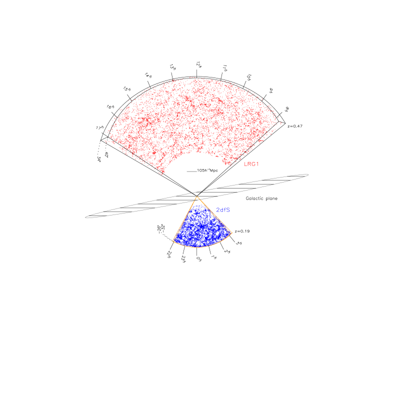
These three samples are important for the detection of the acoustic peak. Although the SDSS-LRG samples are larger and cover a redshift range less affected by nonlinear effects, the lower redshifts mapped by the 2dFVL sample are also important, providing the yardstick that can be compared with the characteristic BAO scales at larger redshifts (see Fig. 1).

Figure 1.— The large slice is drawn from the SDSS-LRG (DR7) survey. The slice is $6^{\circ}$ wide in declination and the galaxy distribution is shown within the redshift range $0.16\leq z\leq 0.47$. There are 10,136 red luminous galaxies within this slice depicted as red dots. The smaller slice with blue dots shows the galaxy distribution of 9,744 objects from the Southern Galactic hemisphere of the 2dFVL sample, reaching a depth of $z=0.19$. To illustrate the scale of the acoustic peak a segment of length $105\,h^{-1}$Mpc is shown to scale.

3. Estimating correlation functions

We estimated the spherically-averaged redshift-space correlation functions by using the Landy-Szalay border-corrected estimator (Landy & Szalay, 1993) that has good large-scale properties. We generated a random distribution of points following the selection function of each catalogue considered, and estimated the correlation function $\xi(s)$.

$$\widehat{\xi}_{\rm{LS}}(s)=1+\frac{DD(s)}{RR(s)}-2\frac{DR(s)}{RR(s)}\,$$ (1)

where $DD(s)$, $RR(s)$ and $DR(s)$ are the probability densities of galaxy-galaxy, random-random and galaxy-random pairs, respectively, for a pair distance $s$. There are several recipes for the choice of the size $N_{\mathrm{rd}}$ of the random point set; as we are interested in large-distance correlations, where the numbers of pairs per bin (kernel width) are large, we used $N_{\rm{rd}}\approx 5N$ ($N$ is the number of galaxies in the sample). Increasing $N_{\rm{rd}}$ up to $20N$ led to pointwise differences less than a percent.

We estimate the probability densities by the kernel method, summing the box spline $B_{3}(\cdot)$ kernels (Saar et al., 2007) centered at each pair distance, and sampling the distributions at smaller intervals than the kernel width.

For the 2dFVL sample, we generated the random catalogues using the subroutines to calculate the completeness and the magnitude limit from the angular masks, both provided by the 2dF team (Colless et al., 2001).

For the DR7-LRG samples we generated the angular mask from the data (as in Hütsi, 2006), following the scan stripes of the survey and defining by hand the rectangles in the survey coordinate system $\eta,\lambda$ that cover the data footprint. We assumed the angular selection to be constant inside this mask.

The DR7-LRG sample is only approximately volume-limited, and we generated the random samples based on the smoothed comoving density of the data. The accepted statistical paradigm for the galaxy distribution is to model it as a Cox process – a Poisson point process where the local intensity is determined by a realization of a random field. The two-stage nature of this process leads to two sources of errors of sample statistics (correlation functions, in our case). The first source is the possible deviation of the realization correlation function from the true one (cosmic variance) and the other source is the discreteness of the point process – how well its correlation function estimate approximates that of the particular realization.

Precise estimates of the cosmological statistics have become actual; Norberg et al. (2008) classifies the error estimates as internal and external, this coincides with our classification. As cosmic variance and discreteness variance are independent, they add for the total variance.

If the random field is Gaussian, as usually assumed, and its expected correlation function and power spectrum are more or less known, the covariance of the correlation function estimate can be found as a convolution of the correlation function itself, or as an integral over the power spectrum squared (see, e.g., Cohn, 2006). This is common for all samples; a rough upper limit is

$$\mathrm{Var}(\widehat{\xi}(r)) < \frac{1}{2\pi^{2}}\frac{1}{Vr^{2}}\int P^{2}(k)\,dk\approx$$

$$\approx 5\cdot 10^{-8}(V/h^{-3}\,\mathrm{Gpc}^{3})^{-1}(r/100\,h^{-1}\,\mathrm{Mpc})^{-2},$$

where the numerical value was obtained by using the Eisenstein & Hu (1998) approximation for the power spectrum, with a Gaussian cutoff at $k=100\,h\,\mathrm{Mpc}^{-1}$ (the real-space scale of about $60\,h^{-1}\mathrm{Mpc}$). The sample volume $V$ and pair distance $r$ in this formula are typical for the DR7-LRG and the baryonic peak; the rms error is about $2\cdot 10^{-4}$ in this case, and about $1.5\cdot 10^{-3}$ for the 2dFVL sample. As we shall see below, this is much smaller than the discreteness error in both cases, and we shall neglect it for the rest of the paper.

The discreteness error can be estimated in several ways. The most attractive of these is bootstrap, that uses only the knowledge inherent in the observed data; the observed sample is repeatedly resampled and the statistics found averaging over these bootstrap samples. The assumption that the observed values are i.i.d. (independent and identically distributed) demands that resampling is done with replacement; this leads to the fact that about 1/3 of sample data is sampled more than once. Bootstrapping has been applied to estimate correlation function errors in cosmology before, first by Barrow et al. (1984), but it is intuitively clear that the bootstrap samples represent a different world, where 1/3 of the galaxies of the original sample coincide (are close pairs). So it has been avoided lately, and other methods (block jackknife, for example) are being used.

The latter is a step in the right direction. The reason why the direct approach to bootstrap correlations fails is that bootstrap estimates can be applied only to smooth functions of sample means (see, e.g. Efron & Tibshirani, 1993; Lahiri, 2003). Only in this case can the estimates be proved to be consistent (approaching the population statistics in the large sample limit). Correlation functions do not belong to this class.

However, there is an elegant way to solve the problem (Lahiri, 2003). Let us take a simple case of a random process $Y(x_{i})$ defined on an onedimensional grid. Then, for studying its correlation function at the lag $k$, create another, two-dimensional process $Z_{2}(x_{i})=(Y(x_{i}),Y(x_{i+k}))$. Averaging over the product of the components of $Z_{2}$ gives us the covariance function.

Generalization of this approach to 3-D point processes involves introducing a fine 3-D grid, and generating a random process $Y(x_{i})$ on the grid by assigning to its vertices values 0 or 1 depending if the grid point (or cell) hosts a point of our point process.

As above, let us create a new multidimensional process $Z_{m}(x_{i})$, a collection of $m$ values of $Y(\cdot)$ at the grid points at a fixed distance interval (bin) from $x_{i}$. The number of points in the bin, if the original cell at $x_{i}$ contains a point (the number of neighbours) can be defined as a simple function of this process, $N(Z_{m}(x_{i}))$. The sample mean of this function is the mean number of neighbours for a given distance bin, proportional to the function $DD(s)$ in Eq. (1). This function can be bootstrapped. Notice that if we consider all possible bins we get a full histogram of neighbours of a sample point. Thus, the natural things to bootstrap are such pointwise histograms – histograms of all the neighbour distances from a given point, and, if needed, histograms of distances of random points from a given sample point. All points carry their histograms; generating a bootstrap realization of a correlation function reduces to selecting a sample of histograms (with replacement), summing them to get the bootstrap realization, and applying, e.g., Eq. (1) to get the bootstrap realization of a sample correlation function. In order to be comparable to the original data, the number of histograms in the sum have to be the same as the number of points in the sample; as usual, about 1/3 of them occur in the sum more than once. Random point pairs should not be bootstrapped, as these are merely a tool for performing volume integrals.

This approach is logical and easy to apply. However, not even these histograms are independent, as required – the locations of sample points are correlated, and this has to be taken into account. The recipe for that is not to bootstrap individual points, but data blocks (Lahiri, 2003). Such a procedure can be proved to give consistent estimates. The size of the block is determined by the correlation length. We shall show below that it is the case.

An unusual (for cosmologists) feature of block bootstrap is that blocks can overlap; in fact, the estimates with overlapping blocks are more efficient than those with non-overlapping blocks.

Numerically, this procedure is much cheaper to apply than that of Barrow et al. (1984). If we have enough core memory, we calculate and store the pair distance probability densities for every sample point, average them for block densities, and sum these for bootstrap realizations. As we do not need to recalculate distances, this bootstrap algorithm is fast. It is straightforward to modify this procedure for pairwise or pointwise weighting.

4. Application to Poisson-Voronoi processes

We demonstrate and check the bootstrap machinery described above on a point field where the correlation function is known exactly – the Poisson-Voronoi process. As this process does not depend on the underlying random field, this is a clean and direct check of the recovery of the discreteness variance.

Following van de Weygaert & Icke (1989), we start from a set of seed points distributed randomly in space (a Poisson point process). The set of all vertices of their Voronoi tessellation defines another (Poisson-Voronoi vertices) point process with a well known numerically tractable two-point correlation function (Heinrich et al., 1998).

We used this process as a testbed for our correlation function estimates and the bootstrap recipes for its variance and bias. For that, we generated 100 samples of Voronoi vertices within the DR7-LRG sample volume, with about the same mean density. We found correlation functions for all these realizations, estimated their bias and variance, and found the symmetric confidence regions.

Figure 2.— Comparison of the sample variability and bootstrap predictions for a Poisson-Voronoi process modelling the galaxy distribution in the DR7-LRG sample volume. The variability of a sample of 100 realizations of the process is shown by color, the 98% confidence region by red and the 80% confidence region by green. The block bootstrap estimates of variance are made on the basis of a single realization (its correlation function is shown by the yellow line), the predicted confidence regions are shown by blue lines (98% confidence) and by errorbars (80% confidence). The figure shows the overall fit of the observed and predicted variability, the inset shows that for a smaller region at a larger scale.

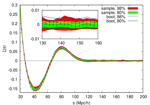
Fig. 2 shows the 98% and 80% confidence regions obtained from these realizations. Then we selected one of these realizations and looked how well the bootstrap procedure predicts the real bias and variance. The predicted variance was the closest to the true one for the block radius $R=15\,h^{-1}$Mpc, which practically coincides with the correlation length ($\xi(R)\approx 1$) for our process. The bootstrap confidence limits are shown in Fig. 2 by the blue lines (for 98%) and by errorbars (for 80%); the variances are easier to compare in the inset. Biases were always considerably smaller than variances, both for the true samples and for the bootstrap samples. Based on these tests, we feel that the bootstrap procedure works well; we shall apply it to the galaxy correlation functions below.

5. Large-scale galaxy correlation functions

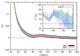
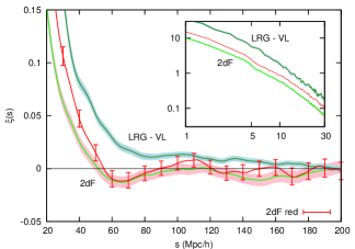
The redshift-space correlation functions for our samples are summarized in Fig. 3. The correlation functions are found as described above, and their errors (biases, variances, confidence regions) are estimated by block bootstrap, with blocks as spheres with the radius $R=12.0\,h^{-1}$ Mpc for the DR7-LRG sample and $R=6.5\,h^{-1}$ Mpc for the 2dFVL sample (the respective correlation lengths). We show in the bottom panel also the correlation function for a subsample of red galaxies from the 2dFVL (chosen according to the spectral type of the galaxy, see Madgwick et al., 2002), with 17,252 galaxies. The block size was chosen the same as for the main sample.

Figure 3.— The redshift space correlation function for the different samples. The top main panel shows the correlation function for the DR7-LRG sample (the 98% and 80% confidence regions in dark red and pale blue and the function as a green line). The acoustic bump is clearly seen at about $105\,\>h^{-1}{\rm{Mpc}}$. The inset shows the large-scale behaviour of the correlation function (multiplied by $s^{2}$). The function is shown by the green line, its 80% confidence region in pale blue, and it is compared with the original BAO discovery data (Eisenstein et al., 2005) with errorbars, labelled by Eis05. Note that the the acoustic peak is wider in the new sample. The bottom panel shows the redshift-space correlation function for the volume-limited samples: for the 2dFVL sample (the 80% confidence region in pink, the function in light green), for the red galaxy subsample of the 2dFVL (the red line with errorbars covering the 80% confidence region), and for the DR7-LRG-VL (the 80% confidence region in pale blue, the function in dark green). The inset shows these correlation functions at short scales. Numerical values of the correlation functions plotted here can be downloaded from http://www.uv.es/martinez.

The top panel shows the correlation function for the DR7-LRG sample. We see that the function $\xi(s)$ remains positive in the whole range shown (up to $200\,\>h^{-1}{\rm{Mpc}}$). It also shows confidently the $105$ $\>h^{-1}{\rm{Mpc}}$ maximum. The inset amplifies the large-distance behaviour of the LRG correlation function. We show the quantity $s^{2}\xi(s)$ for the DR7-LRG and compare it with the correlation function estimates by Eisenstein et al. (2005). We show here only the 80% symmetric confidence region that is comparable with the $\pm\sigma$ limits of the previous estimate. We see that the new data shows the BAO peak with a much better confidence and also reveals that the peak is much wider than the peak found in DR3-LRG. A similar trend was also seen in the analysis by Cabré & Gaztañaga (2009).

The bottom panel shows the 80% confidence level region for the 2dFVL (by pink), and shows the 80% confidence limits for the red galaxies from the 2dFVL by errorbars. In contrast to the DR7-LRG, the correlation function for the 2dFVL sample crosses zero at about $55\,\>h^{-1}{\rm{Mpc}}$ reaching a local minimum with $\xi(s)<0$ at about $65\,\>h^{-1}{\rm{Mpc}}$. At larger scales, this correlation function tends also towards the $105\,\>h^{-1}{\rm{Mpc}}$ maximum. This maximum is present, even more prominently, in the correlation function of the red galaxy subsample. It is precisely at this scale where the LRG sample shows the acoustic baryonic peak first noted by Eisenstein et al. (2005).

The inset shows the behaviour of the correlation function of the volume-limited samples, DR7-LRG VL, 2dFVL, and 2dFVL red, at short scales, characterised by a power-law regime with a downturn at the smallest scales (see, e.g., Ross et al., 2007). The difference in the correlation function amplitudes is a clear fingerprint of the luminosity-color segregation. The LRG galaxies are very luminous red objects lying in more dense environments and displaying enhanced clustering.

6. Conclusions

The results show, first, that the baryon acoustic peak is a stable feature in the large-distance galaxy correlation function. We have presented the analysis of the LRG sample drawn from the last data release (DR7) of the SDSS. This survey is much larger and more compact than the data used before, so edge-correction effects are smaller now and results are therefore more robust. While the peak is most prominent in the distribution of luminous red galaxies (because of the large spatial extent of the sample), it can be seen, if we know what to look for, in smaller galaxy samples. We have reported the first detection of the baryon acoustic peak in a volume-limited sample of very luminous galaxies drawn from the 2dFGRS.

Second, the baryon peak is much wider than found before and than expected; the distortions responsible for that demand careful analysis.

Third, the minimum in the large-distance correlation functions of some samples demands explanation – is it really the signature of voids?

And, fourth, a new internal method to estimate the errors of the correlation function has been introduced. The method is based on a generalization of the application of the bootstrap resampling techniques to smooth functions of sample means.

Acknowledgements

We thank Darren Croton for the 2dfGRS samples and the mask data, Rien van de Weygaert and Dietrich Stoyan for their advise regarding the Voronoi-Poisson process, Robert Lupton for useful discussions and Jun Pan and Jan Hamann for insightful comments on a preliminary draft of this letter.

This work has been supported by the University of Valencia through a visiting professorship for Enn Saar and by the Spanish MEC projects AYA2006-14056 and CSD2007-00060, including FEDER contributions. PAM acknowledges support from the Spanish MEC through a FPU grant. ES and ET acknowledge support by the Estonian Science Foundation, grants No. 6104, 6106, 7146 and by the Estonian Ministry for Education and Science, grant SF0060067s08.

Funding for the SDSS and SDSS-II has been provided by the Alfred P. Sloan Foundation, the Participating Institutions, the National Science Foundation, the U.S. Department of Energy, the National Aeronautics and Space Administration, the Japanese Monbukagakusho, the Max Planck Society, and the Higher Education Funding Council for England. The SDSS Web Site is http://www.sdss.org/.

References

- Abazajian et al. (2008) Abazajian, K. et al. 2008, arXiv:astro-ph/0812.0649
- Barrow et al. (1984) Barrow, J. D., Bhavsar, S. P., & Sonoda, D. H. 1984, MNRAS, 210, 19P
- Cabré & Gaztañaga (2009) Cabré, A., & Gaztañaga, E. 2009, MNRAS, 393, 1183
- Cohn (2006) Cohn, J. D. 2006, New Astronomy, 11, 226
- Cole et al. (2005) Cole, S. et al. 2005, MNRAS, 362, 505
- Colless et al. (2001) Colless, M. et al. 2001, MNRAS, 328, 1039
- Croton et al. (2004) Croton, D. J. et al. 2004, MNRAS, 352, 828
- Efron & Tibshirani (1993) Efron, B., & Tibshirani, R. J. 1993, An introduction to the bootstrap (London: Chapman and Hall)
- Eisenstein et al. (2001) Eisenstein, D. J. et al. 2001, AJ, 122, 2267
- Eisenstein & Hu (1998) Eisenstein, D. J., & Hu, W. 1998, ApJ, 496, 605
- Eisenstein et al. (2005) Eisenstein, D. J. et al. 2005, ApJ, 633, 560
- Heinrich et al. (1998) Heinrich, L., Körner, R., Mehlhorn, N., & Muche, L. 1998, Statistics, 31, 235
- Hütsi (2006) Hütsi, G. 2006, A&A, 449, 891
- Lahiri (2003) Lahiri, S. N. 2003, Resampling Methods for Dependent Data (New York: Springer)
- Landy & Szalay (1993) Landy, S. D., & Szalay, A. S. 1993, ApJ, 412, 64
- Madgwick et al. (2002) Madgwick, D. S. et al. 2002, MNRAS, 333, 133
- Norberg et al. (2008) Norberg, P., Baugh, C. M., Gaztañaga, E., & Croton, D. J. 2008, arXiv:astro-ph/0810.1885
- Percival et al. (2007) Percival, W. J. et al. 2007, ApJ, 657, 51
- Ross et al. (2007) Ross, N. P. et al. 2007, MNRAS, 381, 573
- Saar et al. (2007) Saar, E., Martínez, V. J., Starck, J.-L., & Donoho, D. L. 2007, MNRAS, 374, 1030
- van de Weygaert & Icke (1989) van de Weygaert, R., & Icke, V. 1989, A&A, 213, 1
- Zehavi et al. (2005) Zehavi, I. et al. 2005, ApJ, 621, 22