A chilean seismic regionalization through a Kohonen neural network

Abstract

A study of seismic regionalization for central Chile based on a neural network is presented. A scenario with six seismic regions is obtained, independently of the size of the neighborhood or the reach of the correlation between the cells of the grid. The high correlation between the spatial distribution of the seismic zones and geographical data confirm our election of the training vectors of the neural network.

I Introduction

The idea of seismic regionalization can be traced back to 1941 when Gorshkov urss41 published one of the first studies on seismic regionalization for the URSS. Based on these earlier studies, Richter richter , in a paper entitled “Seismic regionalization”, founded the basis of a methodology that allows to have information dealing with preventing the potential damage that an earthquake may cause through the definition of hazard zones.

In a seismic country like Chile, and based on the urgent goals established by Richter, a proper regionalization map is desirable. Attempts to fill the gap in these matters have been done from time to time. In GL58 is found probably the first regionalization study for Chile where the authors Gajardo and Lomnitz used the same methods of seismic correlation Tsuboi used in the case of Japan. Later works on the subject were mainly focused on engineering aspects as Walkner W64 , Labbe L76 and Barrientos barrientos , discussing on seismic risk. Essentially, these studies used the technique proposed by Cornell C72 and Algermissen and Perkings AyP76 . A more recent study was made by Martin amartin . Here the author used a longitudinal division criteria for the country using the line that separates the deep and superficial earthquakes, which leads to a high degree of coupling between the Nazca and Southamerican plate. This criterium enable him to identify two macro-zones in the continental zone: In the coast, with hypocenters with depths lesser than $40$km, and the mountain macro-zone. As a criteria for latitudinal division, Martin computed the $b$ parameter of the Gutenberg-Richter law for an initial surface, and then he varied the surface iteratively. If $b$ changes dramatically, it means that a seismic zone has been crossed. These are the nine regions Martin found: in the coast; three zones. In the deep mountain zone, he distinguished four zones. In the surface mountain zone, he distinguished a single zone. Finally, the method determined the aseismic zone of Magallanes.

In this work we implement a Kohonen neural network (from here on NN) to determine the seismic zones. In general, a neural network NN can be defined as a computing system made up of a number of simple, highly interconnected processing elements, which processes information by their dynamic state response to external inputs. NNs are typically organized in layers. Layers are made up of a number of interconnected ‘nodes’ which contain an ‘activation function’. Patterns are presented to the network via the ‘input layer’, which communicates one or more ‘hidden layers’ where the actual processing is done through a system of weighted ‘connections’. The hidden layers then link to an ‘output layer’ where the answer is output. Most NNs contain certain types of ‘learning rule’ which modify the weights of the connections according to the input patterns which are exposed to.

In this work we use a special NN appropriated to discriminate spatial distribution. A Kohonen NN KNN (or as it is usually called a self organising map) is an artificial neural network that is trained using unsupervised learning to produce a low-dimensional (typically two dimensional), discretized representation of the input space of the training samples, called a map. The network must be fed a large number of example vectors that represent, as close as possible, the kinds of vectors expected during mapping. The examples are usually provided several times. In this way, the NN finds by itself the best distribution of zones, based on the training vectors, without any other specification than geographical characteristics.

In the context of seismic hazard or seismic risk, there have been many attempts to use this technique. For example, in DTA90 the authors used artificial NN to discriminate between earthquakes and underground nuclear explosions. Also for seismic detection WT95 , in which the NN is trained to recognize signal patterns, and also for earthquake prediction GPR00 . This work is organized as follows. The next section discusses the election of the training vectors or training set, from which the NN starts its learning process. Then, in section III we discusses the way we perform the training process. Section IV is devoted to the analysis of the results and we finish the paper with conclusions.

II Training set

The election of the training set is the crucial step towards the implementation of a useful NN. The usefulness of a NN depends on what we are interested to get from it. As we have discussed in the previous section, the necessity is mainly the one of a hazard categorizer in the Chilean territory. In this section we discuss the criteria in the election of our training set.

II.1 Database

The idea was to associate the earthquake information by zone, frequency and magnitude. We expected the NN finds by itself what we call here ‘zone’, by introducing in it specific information about its seismic history. In this work we use as a database all the earthquakes classified with Richter magnitude equal or larger than $4.5$ Ms in the interval 1957 to 2007. The sources for the data we used, were obtained from the catalog CERESIS ceresis and from the database of the USGS usas (from 1973 to the present).

The area covered by our data set is Chile’s continental territory included inside a rectangle defined around the meridian $72^{\circ}$ W as the North-South axis, between the parallels $17^{\circ}$ S and $56^{\circ}$ S (see the figures for details).

The interval of fifty years ensures us to have a very representative set of data. It is long enough to have earthquake frequency histograms with representative information which could be projected to a larger period of time.

II.2 The Kohonen training vectors

In order to classify the zones, we divided the area selected in the previous section by $156$ rectangular cells of $1^{\circ}\times 1^{\circ}$. Each cell was characterized by a seven dimensional vector, indicating the observed historical seismicity between 1957 to 2007. The $7$D vector is explained below with more details:

$x_{1}$: Mean deep of the seismic sources

$x_{2}$: Number of earthquakes with magnitude $\geq 4.5$ Ms

$x_{3}$: Number of earthquakes with magnitude $\geq 5.5$ Ms

$x_{4}$: Number of earthquakes with magnitude $\geq 6.5$ Ms

$x_{5}$: Maximum observed magnitude

$x_{6}$: Central horizontal coordinate of the cell

$x_{7}$: Central vertical coordinate of the cell

These are considered the minimum number of sensitive parameters which characterize each event. No geophysical input was necessary.

III Training Procedure

The $156$ vectors were introduced into the Kohonen NN. The free parameters in the running are two: the number of iterations and the number of classes or regions. By inspection, it was observed that in all the runnings, and after an average of $2500$ iterations, the NN reached a stable configuration, indicating that the system had found a local minimum.

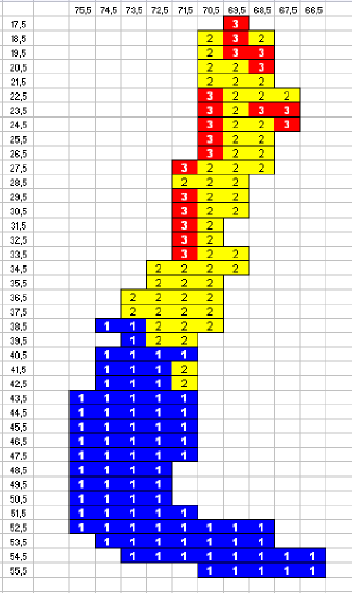
In an initial training session, we forced the NN to create $5$, $10$ and $15$ classes. In all these cases, it was observed that during the first $1000$ iterations, the system reached a stable configuration with just three classes, as it is shown in Fig.(1).

Figure 1: Meta stable configuration after 1000 iterations of the neural network. This result was obtained independent of how many classes we ask for, revealing a strong .

We called these three classes “the fundamental classes”. Let us explain in detail each one of these. According to Fig. (1), in the northern part of the country, we distinguish two classes or two seismic zones of high seismicity, associated to the interaction between the Nazca and South-American plate. In the south, we distinguish another class or seismic zone, with low seismicity, associated to the interaction among the Southamerican, Scotia and Antartic plates.

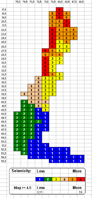
Enhancing the detailed study, we forced the NN to catalog six classes or seismic regions. In this case, after 2500 iterations, the final result was the same, essentially independent of the initial size of the neighborhood. Figure (2) shows the final result using 6 clusters or categories, 2500 iterations and an initial size of the neighborhood of 5.

Figure 2: Transient stable configuration after 2500 iterations and independent of the initial reach of the correlation (or initial size of the neighborhood). The numbers are explained in Table I.

IV Analysis

IV.1 Island regions

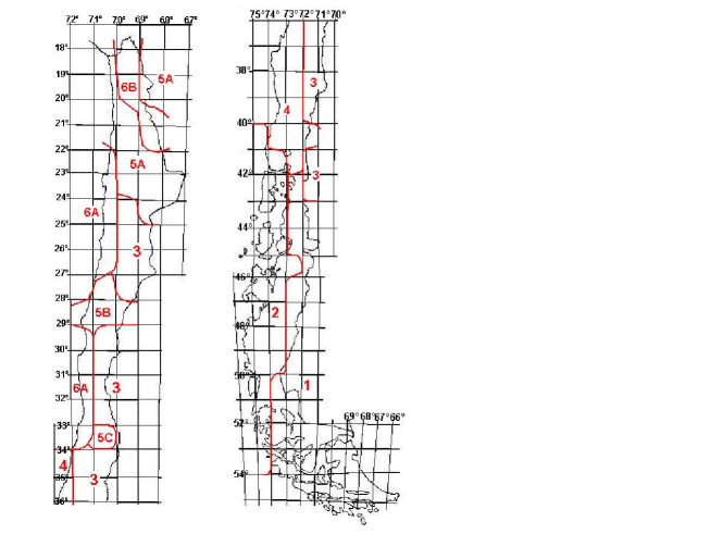
As we can see in Fig.(3), in certain regions some discontinuities occurred, through an interruption of another region. We called these island regions.

In the north part, region 6 becomes separated by two subregions; region 6A (coast) and region 6B (mountain).

The north part, region 5 becomes separated in three subregions; region 5A (including Iquique city), region 5B (including Copiapó city) and region 5C (centered in Santiago city).

Although they are discontinuous regions, the Kohonen NN associates these in the same category because they presented similar seismicity. For that reason we stress to name it just region 5 and 6. Of course, the seismicity associated to each region depends on the chosen vectors representing each cell.

IV.2 Gutenberg-Richter Law

For each region we found the parameters of the Gutenberg-Richter (GR) law. Here $N(\geq M)$ is the mean amount of earthquakes of magnitude larger than $M$ observed in a year, in a normalized area (equivalent to a cell of $1^{\circ}\times 1^{\circ}$ in the equator).

Table 1: This is a summary of the results for the parameters in the Gutenberg-Richter law. The equation reads $\log N=a+bM$, where $M$ is the magnitude in Ms units. It also is given the $\chi^{2}$ of the fit and the maximum magnitude (in Ms units) for each region.

Region	a	b	$\chi^{2}$	Max.Mag. (Ms)	$N(\geq 4.5)$
1	3.844	-1.069	0.9073	5.5	0.11
2	4.209	-0.922	0.8650	6.9	1.15
3	3.298	-0.699	0.9373	7.7	1.42
4	2.702	-0.520	0.9721	8.3	2.30
5	3.784	-0.685	0.9405	7.1	5.02
6	3.702	-0.555	0.9388	7.8	16.03

V Conclusions

Considering the semi-logarithmic GR law slope, we obtain the hierarchy of the six regions, as it is shown in Table II.

Table 2: Here it is displayed the seismic zones under the hierarchy of a growing order according to the $\left|b\right|$ parameter of the Gutenberg-Richter Law. NN used as input data the amount of seisms observed in the last fifty years, we assume that the final hierarchy must be mainly based on the number of earthquakes which are equal or larger than 4.5 Ms, according to Table I.

Hierarchy	Zone	$\left|b\right|$
1	4	0.520
2	6	0.555
3	5	0.685
4	3	0.699
5	2	0.922
6	1	1.069

In Table I, and looking at the first and last columns, we observe the hierarchy based on the seismicity of the zones. As it was explained in section III, the NN was trained with information about the number of earthquakes per range. Then, the definition of seismicity deduced from the NN must be associated to the magnitude and angular orientation of the 7D vectors, which strongly depends on the number of earthquakes equal or larger than $4.5$ Ms.

In this context, zone 1 is an aseismic zone, and zone 6 is the most seismic one.

It is possible that zones 5A and 6B are parts of a larger one extending themselves towards Peru and Bolivia.

The zones 5B and 5C have an interruption between latitudes $29^{\circ}$ and $32^{\circ}$, which coincides with a geographic accident; the intermediate depression despair, being replaced by the fusion between the Andes and coast mountains. Then, zone 5 is strongly associated to the intermediate depression and zone 3 is strongly related to the Andes mountains.

Figure 3: North and South part of Chile. Here is the division of discussed seismic zones in the text.

In the north part of the country, the high seismicity observed can be understood as the result of the activity of the subduction between the Nazca and Southamerican plates (at a rate of convergence of $\sim 10$cm per year, as it is well known).

In the south, we obtain a low seismicity in agreement with the well known result of a convergence of the Southamerican, Scotia and Antartic plates, at a rate of $\sim 2$ cm per year.

In this work we have demonstrated that using a Kohonen NN, and the database available up to date, it can be possible to differentiate six seismic zones for continental Chilean territory. Some of them are apparently disconnected zones (we called these here island zones), but this is in fact an effect produced by considering just an arbitrary portion of territory (that of the political Chilean one) in the analysis. Also, the division between these island zones can be clearly associated with major geographical accidents (as the intermediate depression and some deep valleys) that were not used as input data in the NN. All these facts show the power of using NN analysis in seismic regionalization.

References

- (1) G.P. Gorshkov, Publi. Bureau Central Seismologique International. A19, 25 (1956).
- (2) C.F. Richter, BSSA, 49, 123 (1959).
- (3) E. Gajardo and C. Lomnitz, Seismic province of Chile, Publication 11, 1529 (1958).
- (4) P. Welkner, Estudio de la Sismicidad en Chile y su aplicacion al calculo antisismico, Thesis, Geophysics Department, University of Chile (1964).
- (5) J.C. Labbe, Relaciones macrosismicas para la evaluacion del riesgo sismico en Chile y California, (1976).
- (6) S.E. Barrientos, Regionalizacion Sismica de Chile, M. Sc. Thesis, School of Engineering, University of Chile, 1980.
- (7) C. Cornell, Seism. Soc. Am. Bull., 58, 15831606 (1968).
- (8) S.T. Algermissen and D.M. Perkins, Geolog. Surv. Op.-File Rep. 76-416, (1976).
- (9) A. Martin, Hacia una regionalizacion y calculo del peligro sismico de Chile, Engineering Thesis, School of Engineering, University of Chile, 1990.
- (10) G. Giacinto, R. Paolucci and F. Roli, Pattern Recognition Letters, 18, 1353 (1997).
- (11) M. Sanchez-Silva and L. García, Earthquake Spectra, 17, 89 (2001).
- (12) R. Rojas, Neural Networks - A Systematic Introduction, Springer-Verlag, Berlin, New-York, 1996.
- (13) CERESIS Catalog. Catalogo de terremotos para America del Sur (1985).
- (14) USGS. Web site: http//earthquake.usgs.gov/
- (15) F.U. Dowla, S.R. Taylor and R.W. Anderson, BSSA, 80, 1346 (1990).
- (16) J. Wang and T.-L. Teng, BSSA, 85, 308 (1995); W.-Y. Kim, V. Aharonian, A. L. Lerner-Lam, and P. G. Richards, BSSA, 87, 569 (1997).
- (17) G. Giacinto, R. Paolucci and F. Roli, Pattern Recognition Letters, 18, 1353 (2000).
- (18) T. Kohonen, IEEE Transactions on Computers, Vol. C-21, 353 (1972); T. Kohonen, Self-Organization and Associative Memory, Springer-Verlag, Berlin (1984).