Novel properties in Josephson junctions involving the $\cos(k_{x})\cdot\cos(k_{y})$-pairing state in iron-pnictides

Abstract

We propose a novel trilayer $\pi$-junction that takes advantage of the unconventional $s_{x^{2}y^{2}}=\cos k_{x}\cos k_{y}$ pairing symmetry which changes sign between electron and hole Fermi pockets in the iron-pnictides. In addition, we also present theoretical results for Andreev bound states in thin superconductor-normal metal (or insulator)-iron-pnictide junctions. The presence of non-trivial in-gap states, which uniquely appear in this unconventional pairing state, is a distinct feature in comparison to other singlet pairing states.

A family of iron-based high-temperature superconductors has recently been discovered.kamihara08 These compounds triggered enormous experimental and theoretical interest. In particular, probing the Cooper pair symmetry is critical to understanding the pairing mechanism of this new type of superconductors. Theoretically, many possible gap pairing symmetries have been proposed for iron pnictides, due to the material’s multi-orbital nature and complex Fermi surfaces (FSs), with two hole pockets around $\Gamma$-point and two electron pockets around $M$-point [see Fig. 1 (a)].

Among all the candidates, the proposal of $s$-wave pairing symmetry with relative sign change between hole and electron pockets has appealing advantages.mazin08 ; seo08 ; wang08 ; cvetkovic08 Two of us have predicted,seo08 based on a local magnetic exchange coupling $J_{1}$-$J_{2}$ model,yildirim ; Ma ; si ; Fang2008 an unconventional $s$-wave symmetry with a particular $s_{x^{2}y^{2}}=\cos k_{x}\cos k_{y}$ form in the reciprocal momentum space. The predicted order parameter is consistent with the relative values of the gap on the hole and electron FSs reported by angle-resolved photo-emission spectroscopy (ARPES) experiments.Ding The proposed symmetry is also consistent with low temperature-dependent penetration depth experiments,martin08 ; hashimoto and partially explains nuclear spin-lattice relaxation rate.matano08 ; parish08 However, since most experiments are only sensitive to the magnitude of the gap of superconducting (SC) order, a direct phase-sensitive experiment is essential to map out the complete picture of the pairing symmetry. So far there is no proposed direct phase-sensitive experiment for iron pnictides similar to the dc superconducting quantum interference device (SQUID) interferometer for the cuprates. The difficulty arises from the non-trivial phase structure of the order parameter in $k$ space. One possible phase-sensitive experiment is Andreev spectroscopy in the normal metal to superconductor (NS) junction. Unfortunately, two recent experiments chen08 ; shan08 give seemingly conflicting results and detailed theoretical study shows indistinguishable features between an usual $s$-wave and sign-changed $s$-wave symmetries.linder08

In this paper, we theoretically consider two types of Josephson junctions which have novel properties uniquely associated with a sign-changed $s$-wave SC order as opposed to other (singlet) pairing symmetries. Specifically, the first type of junction we consider is a trilayer SC device where the iron-based superconductor is sandwiched by two other layered, $s$-wave superconductors [see inset of Fig. 1 (b)]. With certain chosen FSs of the two outside layers which couple stronger, respectively, to the hole and electron pockets of the iron pnictide, due to momentum conservation, it is shown that sign-changed $s$-wave pairing symmetry uniquely gives rise to a $\pi$-junction behavior.berg08 ; harlingen95 The second type is a single-band superconductor-normal metal (or insulator)-iron pnictide ($\text{SNS}^{\prime}/\text{SIS}^{\prime}$) junction (see Fig. 2). Based on the similar physics of Andreev reflection at the interface between a normal metal and a superconductor,hu94 ; ghaemi08 we demonstrate that, by adopting a minimal two-orbital model seo08 ; raghu08 to include the multi-orbital effect and complex FSs, the non-trivial phase structure of the sign-changed $s$-wave symmetry shows up in the profile of the quasi-particle (QP) local density of states (LDOS) in the normal region of the junction (see Fig. 4): the sign-changed $s$-wave symmetry state supports in-gap bound state solutions.

$Novel$ $\pi$-$junction$. We propose a composite Josephson junction in which $\pi$-junction behavior can occur based on the unusual phase structure of the $s_{x^{2}y^{2}}$-wave pairing. A $\pi$-junction defines the situation when the Josephson coupling $J$ between two superconductors becomes real and negative (with no spontaneous or explicit time reversal symmetry breaking). In other words, the ground state energy (GSE) is minimized as the phase difference $\Phi$ between two superconductors is “$\pi$”, in contrast to the case of a “0”-junction. The occurrence of the $\pi$-shift behavior can be usually due to magnetic ordering, strong correlation effects near the tunneling interface,berg08 or non-trivial phase structure of the SC order parameter such as $d_{x^{2}-y^{2}}$ pairing symmetry.harlingen95

Figure 1: (Color online) The plots of (a) schematic stacked Fermi surfaces from tri-layer superconducting junction and (b) the ground state energy deviation (from $\Phi=0$ case) per site as a function of relative phase $\Phi$ with $\theta_{m}=0$. The colored curves in (a) represent the FSs of the iron-pnictides.

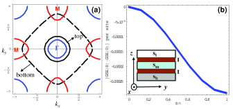
Unlike these common designs, our proposed junction [see the inset of Fig. 1 (b)] is composed of an iron-pnictide ($\text{S}_{m}$) sandwiched by a top and a bottom quasi-2D $s$-wave superconductors ($\text{S}_{t}$ and $\text{S}_{b}$). The interface between any two superconductors is an insulating thin film playing the role of a tunneling barrier. The key requirement for the top and bottom superconducting materials is that the Cooper-pair tunneling probability is stronger into the hole (electron) pockets for the top (bottom) or vice versa. This could be engineered to be due to the normal state FSs of the top and bottom superconductors. One possible way to achieve this condition is to select a small FS and a large FS around $\Gamma$ point for the top layer and the bottom layer, respectively [see Fig. 1 (a)], provided the in-plane (perpendicular to the tunneling direction) momentum is conserved ideally after tunneling.

A simple mean-field model Hamiltonian for this trilayer junction can be of the form, $H_{J}=H_{t}+H_{m}+H_{b}+H_{T}$, where $H_{\eta}=\sum_{\mathbf{k}}\hat{\psi}^{\dagger}_{\eta}[(\varepsilon_{\eta,\mathbf{k}}-\mu)\sigma_{3}+\Delta_{\eta}e^{i\theta_{\eta}}\sigma_{+}+\Delta_{\eta}e^{-i\theta_{\eta}}\sigma_{-}]\hat{\psi}_{\eta}$ for $\eta=t,b$. $\varepsilon_{\eta,\mathbf{k}}$ has the form of $-2t_{\eta}(\cos k_{x}+\cos k_{y})+\epsilon_{\eta}$, $\sigma_{\pm}=(\sigma_{1}\pm i\sigma_{2})/2$, and $\hat{\psi}_{\eta}$ is the usual Nambu spinor, $\hat{\psi}^{\dagger}_{\eta}=(c^{\dagger}_{\eta,\mathbf{k},\uparrow},c_{\eta,-\mathbf{k},\downarrow})$. The difference between the top and bottom SC phases is gauge invariant for the whole junction and is set to be $\Phi=\theta_{t}-\theta_{b}$. $H_{m}$, the Hamiltonian of the iron pnictide, is shown in Eq. (5) transformed into momentum space with band parameters and non-vanishing $\Delta_{s2}=\Delta e^{i\theta_{m}}$ given in the caption of Fig. 3. The tunneling Hamiltonian, $H_{T}$, which connects neighboring layers, takes the simple form: $H_{T}=\sum_{\mathbf{p},\mathbf{k},\eta}\hat{\psi}^{\dagger}_{\eta}(\mathbf{p})\hat{h}_{T,\eta}\hat{\psi}_{m}(\mathbf{k})$, where $\hat{h}_{T,\eta}$ is a $2\times 4$ matrix,

$$\left(\begin{array}[]{cccc}g_{\eta}&0&g_{\eta}&0\\ 0&-g_{\eta}&0&-g_{\eta}\end{array}\right)\delta_{\mathbf{p},\mathbf{k}}$$ (1)

and the spinor $\hat{\psi}^{\dagger}_{m}=(c^{\dagger}_{1,\mathbf{k},\uparrow},c_{1,-\mathbf{k},\downarrow},c^{\dagger}_{2,\mathbf{k},\uparrow},c_{2,-\mathbf{k},\downarrow})$ describes the iron pnictide. Note that we have assumed that the dispersion along $z$-axis is irrelevant and negligible in quasi-2D materials.

For demonstration purpose, we choose parameters $t_{t}=t_{b}=1,\epsilon_{t}=4.78,\epsilon_{b}=1.88$, $g_{t}=g_{b}=0.01$, $\Delta_{t}=0.5,\Delta_{b}=0.4,\Delta=0.5$, and $\theta_{m}=0$. The stacked FSs in the first Brillouin zone from each layer is shown in Fig. 1 (a). Now, it is easy to diagonalize $H_{J}$ and the ground-state energy for this mean-field Hamiltonian is simply the sum of all QP eigen-energies below $E=0$. As presented in Fig. 1 (b), the ground state energy per site relative to the energy of $\Phi=0$ decreases as a function of $\Phi$ with its minimum located at “$\pi$”. The physics of this result can be easily captured by the perturbation calculations of GSE, which give, up to second order of $g^{2}_{\eta}$, $-J_{tm}\cos(\theta_{t}-\theta_{m})-J_{mb}\cos(\theta_{m}-\theta_{b})$, where the Josephson couplings,$J_{tm}>0,J_{mb}<0$ (the sign difference between the Josephson couplings is due to $\pi$ phase difference between electron-like and hole-like FSs), have similar form of the textbook derivation.deGennes It is obvious to see that the global minimum reaches at $|\theta_{t}-\theta_{b}|=\pi$. The overall junction shows “$\pi$” behavior.

Some comments on the experimental realization are in order. First, “large” or “small” FS is meaningful only when the lattice constant $a$ is equal or comparable to the iron pnictides, where the nearest-neighbor Fe-Fe distance is around 2.85Å. Second, to make the tunneling processes reasonably dominated by in-plane momentum conservation, quasi-2D, $s$-wave SC materials should be used for the top and bottom layers due to their irrelevant dispersion along $z$ direction and the epitaxial growing technique may be useful for making the coherent-tunnel interfaces. Based on these considerations, some plausible candidates for the large FS are, for instance, $\text{MgB}_{2}$ from its $\pi$ band with $a\sim 3$Å or thin film of Beryllium with $a\sim 2.3$Å; for the small FS, it could be 2H-$\text{NbSe}_{2}$, where $a\sim 3.45$Å.candidates

Figure 2: (Color online) A schematic plot of the $\text{SNS}^{\prime}$ junction.

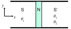
$SNS^{\prime}/SIS^{\prime}$ $junctions$. A further feature of the $s_{x^{2}y^{2}}$-SC is revealed by considering a Josephson junction which connects, on one side, a single-band $s$-wave superconductor, through a normal metal to, on the other side, an iron-based superconductor.linder09 We assume its QP spectrum is well approximated by a BCS type mean-field Hamiltonian subject to an inhomogeneous pairing field along the tunneling direction. Ignoring the $z$-axis for simplicity, the 2D model Hamiltonian of this junction reads,

$$\mathcal{H} = \Theta(-x-\frac{d}{2})H_{S}+\Theta(\frac{d}{2}-|x|)H_{N}+\Theta(x-\frac{d}{2})H_{S^{\prime}}$$ (2)

$$+ H_{T},$$

$$H_{S} = -t_{S}\sum_{\langle\mathbf{r}{\mathbf{r}^{\prime}}\rangle,\sigma}c_{\mathbf{r},\sigma}^{\dagger}c_{{\mathbf{r}^{\prime}},\sigma}-\tilde{\mu}\sum_{\mathbf{r},\sigma}c^{\dagger}_{\mathbf{r},\sigma}c_{\mathbf{r},\sigma}$$ (3)

$$+ \sum_{\mathbf{r}}(\Delta_{s}c^{\dagger}_{\mathbf{r},\uparrow}c^{\dagger}_{\mathbf{r},\downarrow}+h.c.),$$

$$H_{N} = -t_{N}\sum_{\langle\mathbf{r}{\mathbf{r}^{\prime}}\rangle,\sigma}f_{\mathbf{r},\sigma}^{\dagger}f_{{\mathbf{r}^{\prime}},\sigma}+(U-\tilde{\mu})\sum_{\mathbf{r},\sigma}f^{\dagger}_{\mathbf{r},\sigma}f_{\mathbf{r},\sigma},$$ (4)

where $\Theta(x)$ is the Heaviside function, the shifted chemical potential, $\tilde{\mu}=\mu-\epsilon$, guarantees a partially filled band, and $U$ denotes barrier potential. To mimic the iron pnictide FS, we adopt a two-orbital exchange coupling model. seo08 This leads to a somewhat complicated form of $H_{S^{\prime}}=H_{0}+H_{\Delta}$, where we separate it into the band structure and pairing field parts,

$$H_{0} = \sum_{\mathbf{r},\sigma}[-t_{1}c^{\dagger}_{1,\mathbf{r},\sigma}c_{1,\mathbf{r}+\hat{x},\sigma}-t_{2}c^{\dagger}_{1,\mathbf{r},\sigma}c_{1,\mathbf{r}+\hat{y},\sigma}+h.c.]$$

$$+ \sum_{\mathbf{r},\sigma}[-t_{2}c^{\dagger}_{2,\mathbf{r},\sigma}c_{2,\mathbf{r}+\hat{x},\sigma}-t_{1}c^{\dagger}_{2,\mathbf{r},\sigma}c_{2,\mathbf{r}+\hat{y},\sigma}+h.c.]$$

$$+ \sum_{\langle\langle\mathbf{r}{\mathbf{r}^{\prime}}\rangle\rangle}\sum_{\alpha,\sigma}-t_{3}c^{\dagger}_{\alpha,\mathbf{r},\sigma}c_{\alpha,{\mathbf{r}^{\prime}},\sigma}-\mu\sum_{\alpha,\mathbf{r},\sigma}c^{\dagger}_{\alpha,\mathbf{r},\sigma}c_{\alpha,\mathbf{r},\sigma}$$

$$- \sum_{\langle\langle\mathbf{r}{\mathbf{r}^{\prime}}\rangle\rangle}\sum_{\sigma}[t_{4}e^{i\frac{\pi}{2}[(x^{\prime}-x)+(y^{\prime}-y)]}c^{\dagger}_{1,\mathbf{r},\sigma}c_{2,{\mathbf{r}^{\prime}},\sigma}+h.c.],$$

$$H_{\Delta} = [\sum_{\alpha,\mathbf{r}}\Delta_{0}c^{\dagger}_{\alpha,\mathbf{r},\uparrow}c^{\dagger}_{\alpha,\mathbf{r},\downarrow}+\sum_{\alpha,\langle\langle\mathbf{r}{\mathbf{r}^{\prime}}\rangle\rangle}\frac{\Delta_{s2}}{4}c^{\dagger}_{\alpha,\mathbf{r},\uparrow}c^{\dagger}_{\alpha,{\mathbf{r}^{\prime}},\downarrow}$$ (5)

$$+ \sum_{\alpha,\langle\mathbf{r}{\mathbf{r}^{\prime}}\rangle}\frac{\Delta_{d}e^{i\pi(\alpha-1)}}{4}\phi_{\mathbf{r}{\mathbf{r}^{\prime}}}(c^{\dagger}_{\alpha,\mathbf{r},\uparrow}c^{\dagger}_{\alpha,{\mathbf{r}^{\prime}},\downarrow}-c^{\dagger}_{\alpha,\mathbf{r},\downarrow}c^{\dagger}_{\alpha,{\mathbf{r}^{\prime}},\uparrow})$$

$$+ \sum_{\alpha,\langle\mathbf{r}{\mathbf{r}^{\prime}}\rangle}\frac{\Delta_{s1}}{4}(c^{\dagger}_{\alpha,\mathbf{r},\uparrow}c^{\dagger}_{\alpha,{\mathbf{r}^{\prime}},\downarrow}-c^{\dagger}_{\alpha,\mathbf{r},\downarrow}c^{\dagger}_{\alpha,{\mathbf{r}^{\prime}},\uparrow})]+h.c.$$

where $\alpha=1,2$ correspond to $d_{xz}$ and $d_{yz}$ orbitals, respectively, and the hopping parameters are given in Fig. 3. $\langle\langle\mathbf{r}{\mathbf{r}^{\prime}}\rangle\rangle$ represents a next nearest-neighbor pair and $\phi_{\mathbf{r}{\mathbf{r}^{\prime}}}=1(-1)$ as $\mathbf{r}-{\mathbf{r}^{\prime}}=\pm\hat{x}(\hat{y})$. All pairing fields considered in $\mathcal{H}$ are set to be real.realcond $\Delta_{0},\Delta_{s1},\Delta_{s2}$, and $\Delta_{d}$ correspond to intra-orbital on-site, $\cos k_{x}+\cos k_{y}$, $\cos k_{x}\cos k_{y}$, and $\cos k_{x}-\cos k_{y}$ pairing strength, respectively, and inter-orbital pairing is ignored due to its small contribution as discussed in Ref. seo08, . Finally, $H_{T}$ describes the tunneling amplitudes across two interfaces around $\pm d/2$. It can be written as

$$H_{T}=g_{S}\sum_{\sigma}c^{\dagger}_{\mathbf{r}_{L},\sigma}f_{{\mathbf{r}^{\prime}}_{L},\sigma}+g_{S^{\prime}}\sum_{\alpha,\sigma}c^{\dagger}_{\alpha,\mathbf{r}_{R},\sigma}f_{{\mathbf{r}^{\prime}}_{R},\sigma}+h.c.,$$ (6)

where $\mathbf{r}_{L},{\mathbf{r}^{\prime}}_{L}$ ($\mathbf{r}_{R},{\mathbf{r}^{\prime}}_{R}$) are understood to be coordinates across the left (right) interface.

Before proceeding to compute the QP spectrum and the corresponding LDOS, it is important to realize that $\mathcal{H}$ is particle-hole symmetric under $c_{\mathbf{r},\uparrow}\rightarrow c^{\dagger}_{\mathbf{r},\downarrow},c_{\mathbf{r},\downarrow}\rightarrow-c^{\dagger}_{\mathbf{r},\uparrow}$ (for all fermion operators), and hence its spectrum should be symmetric with respect to zero-energy. Taking advantage of the translational symmetry transverse to the tunneling direction $x$, $\mathcal{H}$ can be further decomposed into a sum of 1D Hamiltonians by partially Fourier-transforming along (100) surface ($y$ direction). As a consequence, the whole system is mapped onto an 1D effective lattice in the form of $\mathcal{H}=\sum_{k_{y}}H_{1D}(k_{y})$. Basically, this transformation results in effective chemical potential and pairing fields with $k_{y}$-dependence.

Figure 3: (Color online) QP spectrum in the $\text{SNS}^{\prime}$ junction involving the iron-pnictide with various pairing symmetries. The red line represents Andreev bound states in the case of $s_{x^{2}y^{2}}$-wave pairing. The used parameters are $U=0$, $\tilde{\mu}=-2$, $\Delta_{s}=0.5$, $g_{S}=g_{S^{\prime}}=1$, $t_{1}=-1$, $t_{2}=1.3$, $t_{3}=-0.85$, $t_{4}=-0.85$, $\mu=1.58$, $n_{m}=1$, and the pairing strength is, respectively, (a) $\Delta_{0}=0.5$ (n=201), (b) $\Delta_{s2}=0.5$ (n=201), (c)$\Delta_{s1}=0.5$ (n=201), and (d) $\Delta_{d}=0.5$ (n=601) in energy units, $t_{s}\equiv 1$.

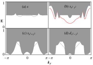
We diagonalize the model Hamiltonian $H_{1D}(k_{y})$ for $-\pi\leq k_{y}<\pi$ on the Nambu basis $\Psi$, where in numerical calculations we take the total number of the $1D$ lattice sites $n$ sufficiently large with open boundary conditions; the normal metal is always set in the middle of system and it is $n_{m}$-site wide. This length is always much less than the SC coherence length. In Fig. 3, we show numerical results of the zero temperature QP spectrum as a function of $k_{y}$ for various pairing symmetries of the iron-pnictides at $\mu=1.58$ (electron doped). In addition, to visualize the Andreev bound states, in Fig. 4 we also compute each corresponding QP-LDOS as a function of position and energy, $D(x,\omega)=\sum_{k_{y},i}|\Psi_{i}(x,k_{y})|^{2}\delta(\omega-\epsilon_{i})$, where $i$ denotes the $i$th eigenfunction. The magnitude of the bulk SC order parameters on both sides of the junction is taken to be the same. The ratio of the gap to the half band-width of the spectrum is around 0.02 and the coherence length is estimated as $\xi\sim v_{F}/\Delta_{s}\sim 4a$.

Figure 4: (Color online) QP-LDOS at $x=0$ in the $\text{SNS}^{\prime}$ junction involving iron-pnictide with various pairing symmetries. The used parameters are the same as in drawing Fig. 3, except that $n=121$ for (a)-(c) and $n=161$ for (d).

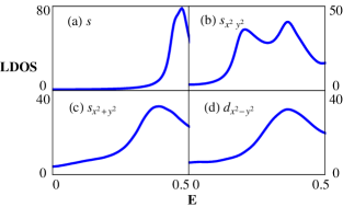
As clearly seen in Fig. 3, the presence of the in-gap Andreev bound states with significant weight in different $k_{y}$ channels for the extended $s$-wave $\cos k_{x}\cos k_{y}$ ($s_{x^{2}y^{2}}$) pairing symmetry is a sharp feature distinguishing it from other pairing symmetries. Although in addition to (gray-color filled) continuum states there are discrete energy levels for $s$, $s_{x^{2}+y^{2}}$, and $d_{x^{2}-y^{2}}$ pairing symmetries, they are either near the maximum gap edge ($s$) or only appear in certain range of $k_{y}$ ( for $s_{x^{2}+y^{2}}$, $d_{x^{2}-y^{2}}$). Especially for the latter case, due to the presence of nodal points on the electron or the hole pockets, the contribution from scattering-state can easily overwhelm that from the bound states and can lead to qualitatively different QP-LDOS from the case of $s_{x^{2}y^{2}}$-wave, where a sharp peak appears at the positive subgap energy.

Furthermore, two observations deserve mentioning. First, the features shown in Figs. 3 and 4 do not change much for different doping levels as long as the doping concentration is not large enough so that the Fermi surfaces pass the nodal line of $\cos k_{x}\cos k_{y}$, i.e., $k_{x}=\pm\pi/2$ and $k_{y}=\pm\pi/2$. Second, if the barrier potential $U$ is greater than the difference between $\mu$ and the band bottom, the normal region becomes insulating. This moves the subgap peak in the $s_{x^{2}y^{2}}$ LDOS closer to the gap edge without destroying it.

Can we understand the presence of such non-trivial bound states for the $s_{x^{2}y^{2}}$-wave pairing in a simple way? A physical insight for this junction involving such an unconventional symmetry can be obtained by treating the bands at the electron and hole pockets in the iron-pnictide as independent of each other.ng08 Consequently, a simple description for the junction based on Bogoliubov-de Gennes (BdG) equations reads:

$$[\hat{H}_{0,\lambda}\sigma_{3}+\Delta_{\lambda}(\mathbf{r})\sigma_{+}+\Delta_{\lambda}^{*}(\mathbf{r})\sigma_{-}]\psi(\mathbf{r})=\epsilon_{\lambda}\psi(\mathbf{r}),$$ (7)

where $\lambda=1,2$ are the band indices, and $\sigma_{i}(i=1,2,3)$ are the Pauli matrices with $\sigma_{\pm}=(\sigma_{1}\pm i\sigma_{2})/2$ acting in the Nambu space, $\psi=[\tilde{u}_{\lambda}(\mathbf{r}),\tilde{v}_{\lambda}(\mathbf{r})]^{t}$. $\hat{H}_{0,\lambda}$ contains the band information of non-interacting electrons and $\Delta_{\lambda}(\mathbf{r})$ corresponds to the pairing field in the same band $\lambda$. Along the tunneling direction $x$, the inhomogeneous $\Delta_{\lambda}(\mathbf{r})$ is modeled by $\Delta_{\lambda}(x)=\Delta_{s}e^{i\theta_{s}}$ as $x<0$ and $\Delta_{\lambda}(x)=\Delta_{\lambda}e^{i\theta_{\lambda}}$ as $x>0$. For simplicity, we set $\theta_{s}=0$ hereafter and keep in mind that for the sign-changed $s$-wave symmetry, $\theta_{1}=\theta_{2}+\pi$. For electrons near FSs, it is valid to linearize BdG equations within WKJB approximation, $\psi\sim e^{i\mathbf{k}_{F}\cdot\mathbf{r}}\phi(\mathbf{r})$, $\phi(\mathbf{r})=(u(\mathbf{r}),v(\mathbf{r}))^{t}$ and then the BdG equations are now reduced to the form of 1D Dirac equation if we further take the advantage of translational symmetry in transverse direction,

$$[-iv_{Fx}\partial_{x}\sigma_{3}+\Delta_{\lambda}(x)\sigma_{+}+\Delta_{\lambda}^{*}(x)\sigma_{-}]\phi(x)=\epsilon_{\lambda}\phi(x).$$ (8)

After straightforward calculations with trial bound state solutions, $u(v)\sim u_{0}(v_{0})e^{-\gamma_{\pm}x}$, as studied in Ref. ng08, , the discrete energy level within the gap is given by $E_{0}=\pm(\Delta_{s}\Delta_{\lambda}\sin\theta_{\lambda})/\sqrt{\Delta_{s}^{2}+\Delta_{\lambda}^{2}-2\cos\theta_{\lambda}\Delta_{s}\Delta_{\lambda}}$, provided $\cos\theta_{\lambda}<$ min($\Delta_{\lambda}/\Delta_{s},\Delta_{s}/\Delta_{\lambda}$). The pair of solutions with eigenvalues symmetric with respect to zero-energy follows from the particle-hole symmetry of the BdG equations. It is clear to see that when superconductors on both sides of the junction are in phase ($\theta_{\lambda}=0$) no bound state solution is found, while when they are out of phase ($\theta_{\lambda}=\pi$) there are doubly-degenerate zero modes.ng08

The significance of this simple result is that as long as $\theta_{1}=0$ (or $\theta_{2}=0$), there are always zero modes trapped in the normal region of the junction involving iron pnictides with sign-changed $s$-wave pairing symmetry. However, in a more realistic system with band structure such as our $\text{SNS}^{\prime}$ junction it usually introduces finite effective mass for the band electrons, which destroys the validity of using linearized Eq. (8) (where the effective mass goes to infinity). As a result, the to-be-degenerate zero modes split tsai08 as we see in Fig. 3 (only $E>0$ shown). The same argument is also applicable when we further consider the effect brought by $k_{y}$ in our $H_{1D}(k_{y})$.

$Acknowledgements$. We thank E. Berg and C. Fang for stimulating and useful discussions. JPH and WFT are supported by NSF Grant No. PHY-0603759 and DXY is supported by NSF Grand No. DMR-0804748.

References

- (1) Y. Kamihara et al., J. Am. Chem. Soc. 130, 3296 (2008).
- (2) K. Seo, B. A. Bernevig, and J. Hu, Phys. Rev. Lett. 101, 206404 (2008).
- (3) I. I. Mazin et al., Phys. Rev. Lett. 101, 057003 (2008).
- (4) F. Wang et al., Phys. Rev. Lett. 102, 047005 (2009) and references therein.
- (5) V. Cvetkovic and Z. Tesanovic, Europhys. Lett. 85, 37002 (2009).
- (6) T. Yildirim, Phys. Rev. Lett. 101, 057010 (2008).
- (7) F. Ma Z.-Y. Lu, and T. Xiang, Phys. Rev. B 78, 224517 (2008).
- (8) Q. Si and E. Abrahams, Phys. Rev. Lett. 101, 076401 (2008).
- (9) C. Fang et al, Phys. Rev. B 77, 224509 (2008).
- (10) H. Ding et al, Europhys. Lett. 83, 47001 (2008); L. Wray et al, Phys. Rev. B 78, 184508 (2008); L. Zhao et al, Chin. Phys. Lett. 25, 4402 (2008).
- (11) C. Martin et al., arXiv:0807.0876.
- (12) K. Hashimoto et al., Phys. Rev. Lett. 102, 017002 (2009).
- (13) M. M. Parish, J. Hu, and B. A. Bernevig, Phys. Rev. B 78, 144514 (2008).
- (14) K. Matano et al., Europhys. Lett. 83, 57001 (2008); H.-J. Grafe et al., Phys. Rev. Lett. 101, 047003 (2008); Y. Nakai et al., J. Phys. Soc. Jpn. 77, 073701 (2008).
- (15) T. Y. Chen et al., Nature 453, 1224 (2008).
- (16) L. Shan et al., Europhys. Lett. 83, 57004 (2008).
- (17) J. Linder and A. Sudbo, Phys. Rev. B 79, 020501(R) (2009).
- (18) See E. Berg, E. Fradkin, and S. A. Kivelson, Phys. Rev. B 79, 064515 (2009) and references therein.
- (19) D. J. Van Harlingen, Rev. Mod. Phys. 67, 515 (1995).
- (20) C.-R. Hu, Phys. Rev. Lett. 72, 1526 (1994); S. Kashiwaya and Y. Tanaka, Rep. Prog. Phys. 72, 1641 (2000), and references therein.
- (21) P. Ghaemi, F. Wang, and A. Vishwanath, Phys. Rev. Lett. 102, 157002 (2009).
- (22) S. Raghu et al., Phys. Rev. B 77, 220503(R) (2008).
- (23) P. G. de Gennes, Superconductivity of Metals and Alloys (Addison-Wesley, New York, 1989).
- (24) For instance, see J. Kortus et al., Phys. Rev. Lett. 86, 4656 (2001); A. E Curzon et al., J. Phys. C 2 382 (1969); T. Yokoya et al., Science 294, 2518 (2001).
- (25) Using a similar SNS’ junction, 0- oscillations in the Josephson current have been found by J. Linder, I. B. Sperstad, and A. Sudb , Phys. Rev. B 80, 020503(R) (2009).
- (26) We neglect the possibility of a spontaneously time reversal symmetry broken ground state.
- (27) T. K. Ng and N. Nagaosa, arXiv:0809.3343.
- (28) W.-F. Tsai et al., unpublished note.