Neutrino masses and mixing, lightest neutralino decays and a solution to the μ𝜇\mu problem in supersymmetry

Pradipta Ghosh and Sourov Roy
Department of Theoretical Physics and Centre for Theoretical Sciences,
Indian Association for the Cultivation of Science,
2A &\& 2B Raja S.C. Mullick Road, Kolkata 700 032, India
E-mails:
tppg@iacs.res.in, tpsr@iacs.res.in
Abstract:

We examine in detail the neutrino masses and mixing patterns in an extension of the minimal supersymmetric standard model with three gauge-singlet neutrinos and R-parity violation. The Majorana masses for the gauge-singlet neutrinos as well as the usual μ𝜇\mu-term for the Higgs superfields are generated at the electroweak scale through the vacuum expectation values of the singlet sneutrinos. The resulting effective mass matrix for the three light neutrinos have contributions from the seesaw mechanism involving the singlet neutrinos as well as due to the mixing with the heavy neutralinos. This model is popularly known in the literature as the “μ𝜇\mu from ν𝜈\nu supersymmetric standard model” (μν𝜇𝜈\mu\nuSSM). We show that even with flavour diagonal neutrino Yukawa couplings, the global data on three-flavour neutrinos can be well accounted for in this scenario, at the tree level. We also analyze the mixing in the chargino and the Higgs sector and calculate the decays of the lightest supersymmetric particle in this model. The decay branching ratios show certain correlations with the neutrino mixing angles, which can be tested at the LHC. Some other phenomenological implications of such a model have been discussed.

Supersymmetry Phenomenology

1 Introduction

The experimental results on neutrinos provide strong evidence in favour of non-zero neutrino masses and mixing angles. Various neutrino oscillation experiments suggest that the mixing pattern of the three light neutrinos is bilarge, that is to say there are two large mixing angles and one small mixing angle. The data can be explained very well with the following set of mass squared differences and mixing angles [1, 2]

7.05×10⁵eV2Δm2128.34×105eV2(3σ),formulae-sequence7.05superscript105superscripteV2Δsubscriptsuperscript𝑚2218.34superscript105superscripteV23𝜎\displaystyle 7.05\times 10^{-5}{\rm eV}^{2}\leq\Delta m^{2}_{21}\leq 8.34\times 10^{-5}{\rm eV}^{2}~{}~{}~{}~{}~{}~{}~{}~{}(3\sigma), (1)
2.07×10³eV2|Δm312|2.75×10³eV2(3σ),formulae-sequence2.07superscript103superscripteV2Δsubscriptsuperscript𝑚2312.75superscript103superscripteV23𝜎\displaystyle 2.07\times 10^{-3}{\rm eV}^{2}\leq|\Delta m^{2}_{31}|\leq 2.75\times 10^{-3}{\rm eV}^{2}~{}~{}~{}~{}~{}~{}(3\sigma), (2)
30θ1237,35θ2354,θ1313(3σ),formulae-sequencesuperscript30subscript𝜃12superscript37superscript35subscript𝜃23superscript54subscript𝜃13superscript133𝜎\displaystyle 30^{\circ}\leq{\theta_{12}}\leq 37^{\circ},~{}35^{\circ}\leq{\theta_{23}}\leq 54^{\circ},~{}{\theta_{13}}\leq 13^{\circ}~{}~{}~{}~{}~{}~{}(3\sigma), (3)

where Δmij2mi2mj2Δsubscriptsuperscript𝑚2𝑖𝑗subscriptsuperscript𝑚2𝑖subscriptsuperscript𝑚2𝑗\Delta m^{2}_{ij}\equiv m^{2}_{i}-m^{2}_{j}.

In order to explain the results in eqs.(1)– (3), one needs to go to a theory beyond the standard model (SM). A very interesting possibility to look for new physics is supersymmetry (SUSY) which has the ability to provide a solution of the so-called ‘gauge hierarchy problem’ connected with the mass of the Higgs boson. SUSY predicts new particles at the TeV scale which can be tested at the forthcoming Large Hadron Collider (LHC). Naturally it is tempting to see whether TeV scale SUSY is also one of the candidates which can explain the observed pattern of neutrino mass squared differences and mixing. There have been several proposals in recent times, which attempt to explain the experimental data on neutrinos in the context of a supersymmetric theory. Perhaps the most well studied class of models in this context is the one which includes R-parity violation [3, 4] in the Minimal Supersymmetric Standard Model (MSSM). Neutrino mass squared differences and mixing angles have been calculated under various assumptions and it has been found that the neutrino data can be explained well when contributions to the neutrino mass matrix at the tree and one-loop level are considered [5, 6].

On the other hand, though SUSY provides some elegant solutions to accommodate the experimental data on neutrinos, it has been plagued by a few urgent questions which do not have very satisfactory answers yet. One of them is the so-called “μ𝜇\mu-problem”[7] related to the bilinear term μH^1H^2𝜇subscript^𝐻1subscript^𝐻2\mu{\hat{H}}_{1}{\hat{H}}_{2} in the MSSM superpotential. The electroweak symmetry breaking requires the value of μ𝜇\mu to be roughly of the order of a few hundreds of GeV. This requires, in the absence of any fine cancellation, that μ𝜇\mu is roughly of the order of the soft scalar masses and both of them should be somewhere around a TeV or a few hundreds of GeV. Since μ𝜇\mu parameter respects SUSY, there is no obvious reason why it should be of the same order as SUSY breaking soft scalar masses. This defines the “μ𝜇\mu-problem”. There have been several attempts to address the solution to this problem and all of them requires the vacuum expectation value(s) (VEVs) of some additional field(s) to generate the μ𝜇\mu-term after the symmetry breaking.

One of the solutions is the next-to-minimal supersymmetric standard model (NMSSM), which introduces a superfield S^^𝑆\hat{S}, singlet under the SM gauge group. The μ𝜇\mu term is absent from the superpotential and it arises when the scalar component of S^^𝑆\hat{S} acquires a VEV. This VEV is determined in terms of the soft supersymmetry breaking terms through the minimization condition. If the SUSY breaking scale is close to the electroweak (EW) scale then the effective μ𝜇\mu term is also of the order of the EW scale. However, as in the case of MSSM, the NMSSM also cannot explain the observed pattern of neutrino masses and mixing.

It is also important to note in this context, that another very well known mechanism of generating small neutrino masses and bilarge mixing angles in a SUSY model, compatible with the experimental data, is the seesaw mechanism which introduces gauge singlet neutrino superfields. In such cases the MSSM superpotential contains additional terms involving the Yukawa couplings for neutrinos as well as Majorana masses for the gauge singlet neutrinos. In the conventional scenario, the neutrino Yukawa couplings are assumed to be 𝒪similar-toabsent𝒪\sim{\cal O}(1), whereas the Majorana masses for the gauge singlet neutrinos are taken somewhere around 1014superscript101410^{14} GeV or so. In this case light neutrino masses as small as 102superscript10210^{-2} eV can be generated. One viable alternative to the usual seesaw mechanism is to consider the TeV-scale seesaw. This possibility is very interesting since it may provide a direct way to probe the gauge singlet neutrino mass scale at the LHC and does not need to introduce a very high energy scale in the theory. However, in order to generate small active neutrino masses one needs to consider neutrino Yukawa couplings to be of order 106superscript10610^{-6}. This choice is reasonable since we know that the electron Yukawa coupling should also be of the order of 106superscript10610^{-6}.

In this work we study in details, a model of neutrino masses and mixing which introduces the gauge singlet neutrino superfields (ν^icsubscriptsuperscript^𝜈𝑐𝑖{\hat{\nu}}^{c}_{i}) to solve the μ𝜇\mu problem in a way similar to that of NMSSM. The terms in the superpotential involving the ν^icsubscriptsuperscript^𝜈𝑐𝑖{\hat{\nu}}^{c}_{i} include the neutrino Yukawa couplings, the trilinear interaction terms among the singlet neutrino superfields as well as a term which couples the Higgs superfields to the ν^icsubscriptsuperscript^𝜈𝑐𝑖\hat{\nu}^{c}_{i}. In addition, there are corresponding soft SUSY breaking terms in the scalar potential. When the scalar components of ν^icsubscriptsuperscript^𝜈𝑐𝑖{\hat{\nu}}^{c}_{i} get VEVs through the minimization conditions of the scalar potential, an effective μ𝜇\mu term with an EW scale magnitude is generated [8]. In addition, small Majorana masses of the active neutrinos are generated due to the mixing with the neutralinos as well as due to the seesaw mechanism involving the gauge singlet neutrinos. In such a scenario, we aim to explain the experimental data on neutrinos discussed in the beginning. In particular, we show that it is possible to provide a theory of neutrino masses and mixing explaining the experimental data, even with a flavour diagonal neutrino Yukawa coupling matrix, without resort to an arbitrary flavour structure in the neutrino sector. This essentially happens because of the mixing involved in the neutralino-neutrino (both doublet and singlet) system mentioned above. We perform a detailed analytical and numerical work and show that the three flavour neutrino data can be accommodated in such a scenario. In addition, we observe that in this model different neutrino mass hierarchies can also be obtained with correct mixing pattern, at the tree level.

In this model the neutral Higgs bosons mix with the sneutrinos and charged Higgs bosons mix with the charged sleptons. The corresponding scalar, pseudoscalar and charged scalar mass squared matrices are enlarged and we take into account the constraints on the parameters coming from the positivity of the squared scalar masses. In the fermionic sector, in addition to the neutralino-neutrino mixing there is mixing also between the charginos and the charged leptons. This can also have implications for phenomenological studies, particularly in the context of future colliders. Because of the mixing between the neutralinos and the neutrinos, the lightest neutralino, which is the lightest superparticle (LSP) for most of the parameter space, can have novel decay modes which can be correlated with the neutrino mixing pattern. This can provide some unique signatures of such a scenario which can be tested at the LHC.

As we have mentioned earlier, that in order to get the correct light neutrino mass scales, the neutrino Yukawa couplings should be of the order of 106superscript10610^{-6} or so. This is because the TeV scale VEVs of the singlet neutrinos induce Majorana mass terms of themselves also at the TeV scale. Similarly, the neutralino-neutrino mixing provides correct light neutrino mass scales only when the Yukawa couplings of the neutrinos are somewhere close to that of the electron. This model has been named as the “μν𝜇𝜈\mu\nuSSM” in ref.[8]. Thus in this model, an interesting proposal has been given, where the generation of small neutrino masses and the solution to the μ𝜇\mu problem can be accommodated with the same set of gauge singlet neutrino superfields without introducing an extra singlet such as in the case of NMSSM. The spectrum and parameter space of this model, with three gauge singlet neutrino superfields, were discussed in [9]. However, a detailed discussion of the issue of neutrino masses and bilarge neutrino mixing, in order to accommodate the three flavour neutrino data, has been lacking and that is what we want to provide in the present work. We would like to emphasize here that our analysis shows that even with flavour diagonal neutrino Yukawa couplings, the resulting structure of the effective mass matrix of the light neutrinos can explain the bilarge pattern of mixing. In addition, we explore the correlation between neutrino mixing and the decay pattern of the LSP in this model and discuss some other interesting phenomenological implications.

Other models which address the neutrino experimental data and the μ𝜇\mu problem are essentially extensions of NMSSM. One of these proposals [10] include both the gauge singlet neutrino superfields (ν^icsubscriptsuperscript^𝜈𝑐𝑖{\hat{\nu}}^{c}_{i}) and the extra singlet (S^^𝑆\hat{S}) of the NMSSM. In this case the Majorana masses of the singlet neutrinos are also generated at the EW scale through the VEV of the scalar component of S^^𝑆\hat{S}. R-parity may be broken spontaneously and the light neutrino masses are generated through the seesaw at the EW scale. Another possibility is discussed in ref.[11], where the effective bilinear R-parity violating terms are generated through the VEV of the singlet scalar S𝑆S. Naturally, in this case only one neutrino mass is generated at the tree level whereas the other two masses are generated at the loop level. In [12], two neutrino masses are generated at the tree level by including explicit bilinear R-parity violating terms in addition to the R-parity breaking term involving S^^𝑆\hat{S}.

The plan of the paper is the following. We start with the description of the model in Sec. II by writing down the superpotential and the soft supersymmetry breaking interaction terms. We also derive the minimization equations of the scalar potential and discuss some issues related to the vacuum expectation values of the left sneutrinos. In Sec. III we continue our discussion of the scalar sector with a more detailed look. Sec. IV describes the fermionic sector of the model where neutralinos mix with both the doublet and singlet neutrinos and the charginos mix with the charged leptons. In Sec. V we provide a detailed discussion of the effective mass matrix of the three light neutrinos, arising because of the neutralino-neutrino mixing. Analytical expressions of the mass eigenvalues and eigenvectors are derived under certain conditions, using degenerate perturbation theory. We construct the neutrino mixing matrix and show that it is possible to have two large and one small mixing angles in general. A detailed numerical analysis has been performed and we compare our results with that obtained using the approximate analytical formulae. We show that for realistic parameter choices, it is possible to fit the three flavour global neutrino data in this scenario, even with a flavour diagonal neutrino Yukawa coupling matrix. The decays of the lightest supersymmetric particle are discussed in Sec. VI and it has been observed that certain decay branching ratios are correlated with the neutrino mixing angles. We make concluding remarks in Sec. VII with possible future directions of our work. The details of various scalar mass squared matrices and the Feynman rules for the LSP decay calculations are relegated to the appendices.

2 The model and its minima

2.1 Superpotential

In this section we introduce the model along the lines of ref.[8], discuss its basic features and set our notations. We introduce three gauge singlet neutrino superfields, ν^icsuperscriptsubscript^𝜈𝑖𝑐{\hat{\nu}}_{i}^{c} (i=e,μ,τ𝑖𝑒𝜇𝜏i=e,{\mu},{\tau}), in addition to the fields of the minimal supersymmetric standard model. The superpotential of the model is written as

W𝑊\displaystyle W =\displaystyle= ϵab(YuijH^2bQ^iau^jc+YdijH^1aQ^ibd^jc+YeijH^1aL^ibe^jc+YνijH^2bL^iaν^jc)subscriptitalic-ϵ𝑎𝑏subscriptsuperscript𝑌𝑖𝑗𝑢subscriptsuperscript^𝐻𝑏2subscriptsuperscript^𝑄𝑎𝑖subscriptsuperscript^𝑢𝑐𝑗subscriptsuperscript𝑌𝑖𝑗𝑑subscriptsuperscript^𝐻𝑎1subscriptsuperscript^𝑄𝑏𝑖subscriptsuperscript^𝑑𝑐𝑗subscriptsuperscript𝑌𝑖𝑗𝑒subscriptsuperscript^𝐻𝑎1subscriptsuperscript^𝐿𝑏𝑖subscriptsuperscript^𝑒𝑐𝑗subscriptsuperscript𝑌𝑖𝑗𝜈subscriptsuperscript^𝐻𝑏2subscriptsuperscript^𝐿𝑎𝑖subscriptsuperscript^𝜈𝑐𝑗\displaystyle\epsilon_{ab}(Y^{ij}_{u}\hat{H}^{b}_{2}\hat{Q}^{a}_{i}\hat{u}^{c}_{j}+Y^{ij}_{d}\hat{H}^{a}_{1}\hat{Q}^{b}_{i}\hat{d}^{c}_{j}+Y^{ij}_{e}\hat{H}^{a}_{1}\hat{L}^{b}_{i}\hat{e}^{c}_{j}+Y^{ij}_{\nu}\hat{H}^{b}_{2}\hat{L}^{a}_{i}\hat{\nu}^{c}_{j}) (4)
\displaystyle- ϵabλiν^icH^1aH^2b+13κijkν^icν^jcν^kc,subscriptitalic-ϵ𝑎𝑏superscript𝜆𝑖subscriptsuperscript^𝜈𝑐𝑖subscriptsuperscript^𝐻𝑎1subscriptsuperscript^𝐻𝑏213superscript𝜅𝑖𝑗𝑘subscriptsuperscript^𝜈𝑐𝑖subscriptsuperscript^𝜈𝑐𝑗subscriptsuperscript^𝜈𝑐𝑘\displaystyle\epsilon_{ab}\lambda^{i}\hat{\nu}^{c}_{i}\hat{H}^{a}_{1}\hat{H}^{b}_{2}+\frac{1}{3}\kappa^{ijk}\hat{\nu}^{c}_{i}\hat{\nu}^{c}_{j}\hat{\nu}^{c}_{k},

where H^1subscript^𝐻1\hat{H}_{1} and H^2subscript^𝐻2\hat{H}_{2} are the down-type and up-type Higgs superfields, respectively. The Q^isubscript^𝑄𝑖\hat{Q}_{i} are doublet quark superfields, u^jcsubscriptsuperscript^𝑢𝑐𝑗{\hat{u}}^{c}_{j} [d^jcsubscriptsuperscript^𝑑𝑐𝑗{\hat{d}}^{c}_{j}] are singlet up-type [down-type] quark superfields. The L^isubscript^𝐿𝑖\hat{L}_{i} are the doublet lepton superfields, and the e^jcsubscriptsuperscript^𝑒𝑐𝑗{\hat{e}}^{c}_{j} are the singlet charged lepton superfields. Here a,b𝑎𝑏a,b are SU(2) indices, and ϵ12subscriptitalic-ϵ12\epsilon_{12} = –ϵ21subscriptitalic-ϵ21\epsilon_{21} = 1. Note that the usual bilinear μ𝜇\mu-term of the MSSM is absent from the superpotential whereas two additional trilinear terms are introduced involving the Higgs superfields, H^1subscript^𝐻1\hat{H}_{1} and H^2subscript^𝐻2\hat{H}_{2}, and the three gauge singlet neutrino superfields, ν^icsubscriptsuperscript^𝜈𝑐𝑖\hat{\nu}^{c}_{i}. This is done by imposing a Z3subscript𝑍3Z_{3} symmetry which is also used in the case of NMSSM. If the scalar potential of the model is such that non-zero vacuum expectation values of the scalar components (ν~icsubscriptsuperscript~𝜈𝑐𝑖\tilde{\nu}^{c}_{i}) of the singlet superfields ν^icsubscriptsuperscript^𝜈𝑐𝑖\hat{\nu}^{c}_{i} are induced, an effective bilinear term μH^1aH^2b𝜇subscriptsuperscript^𝐻𝑎1subscriptsuperscript^𝐻𝑏2\mu\hat{H}^{a}_{1}\hat{H}^{b}_{2} is generated, where the coefficient μλiν~ic𝜇superscript𝜆𝑖delimited-⟨⟩subscriptsuperscript~𝜈𝑐𝑖\mu\equiv\lambda^{i}\langle\tilde{\nu}^{c}_{i}\rangle. In the presence of soft supersymmetry breaking, it is usually expected that the VEVs of ν~icsubscriptsuperscript~𝜈𝑐𝑖\tilde{\nu}^{c}_{i} are at the electroweak scale. Hence the value of μ𝜇\mu is of the order of the electroweak scale as long as the dimensionless couplings λisubscript𝜆𝑖\lambda_{i} are 𝒪similar-toabsent𝒪\sim\cal O(1). This gives us a solution to the so-called “μ𝜇\mu-problem”. The last term in the superpotential with the coefficient κijksuperscript𝜅𝑖𝑗𝑘\kappa^{ijk} is included in order to avoid an unacceptable axion associated to the breaking of a global U(1)U1\rm U(1) symmetry [13]. This term generates effective Majorana masses for the singlet neutrinos at the electroweak scale.

The last two terms in (4) explicitly break lepton number (L) and hence the R-parity, which is defined by R=(1)L+3B+2s𝑅superscript1𝐿3𝐵2𝑠R=(-1)^{L+3B+2s}. Here B is the baryon number and s is the spin. Note that R=+1𝑅1R=+1 for particles and 11-1 for superpartners. Since lepton number is explicitely broken, no unwanted massless Majoron appears in this model. One should also notice that the term in the superpotential involving the neutrino Yukawa couplings Yνijsubscriptsuperscript𝑌𝑖𝑗𝜈Y^{ij}_{\nu}, generate effective bilinear R-parity violating interactions ϵiH^2L^isuperscriptitalic-ϵ𝑖subscript^𝐻2subscript^𝐿𝑖\epsilon^{i}\hat{H}_{2}\hat{L}_{i}. Here ϵisuperscriptitalic-ϵ𝑖\epsilon^{i} is determined in terms of the VEVs of ν~icsubscriptsuperscript~𝜈𝑐𝑖{\tilde{\nu}}^{c}_{i} and is given by ϵi=Yνijν~jcsuperscriptitalic-ϵ𝑖superscriptsubscript𝑌𝜈𝑖𝑗delimited-⟨⟩subscriptsuperscript~𝜈𝑐𝑗\epsilon^{i}=Y_{\nu}^{ij}\langle\tilde{\nu}^{c}_{j}\rangle. R-parity breaking implies that the lightest supersymmetric particle (LSP) is not stable and it cannot be a candidate for dark matter. The decay of the LSP may produce some interesting signatures at the LHC, which can have certain correlations with the neutrino oscillation data. In addition, one can measure displaced vertices originating from the LSP decay.

It should be mentioned here that neutrino masses and bilarge neutrino mixing have also been studied in an R-parity violating supersymmetric theory with gauge singlet neutrino superfields [14]. However, in that analysis terms of the type ν^cH^1H^2superscript^𝜈𝑐subscript^𝐻1subscript^𝐻2{\hat{\nu}}^{c}{\hat{H}}_{1}{\hat{H}}_{2} have been dropped from the superpotential because of very small coefficient. Analysis has also been carried out in the context of the observed baryon asymmetry of the Universe [15]. Finally, one should note that the discrete Z3subscript𝑍3Z_{3} symmetry of the superpotential is spontaneously broken in the vacuum. This might lead to cosmological domain wall problem [16]. However, the solutions to this problem exist [17] and will also work in this case.

2.2 Soft terms

Let us now specify the soft-supersymmetry-breaking terms of this model. We will confine ourselves in the framework of supergravity mediated supersymmetry breaking. The Lagrangian softsubscriptsoft\mathcal{L}_{\text{soft}}, containing the soft-supersymmetry-breaking terms is given by

softsubscriptsoft\displaystyle-\mathcal{L}_{\text{soft}} =\displaystyle= (mQ~2)ijQ~iaQja~+(mu~c2)iju~icu~jc+(md~c2)ijd~icd~jc+(mL~2)ijL~iaLja~superscriptsuperscriptsubscript𝑚~𝑄2𝑖𝑗subscriptsuperscript~𝑄superscript𝑎𝑖~subscriptsuperscript𝑄𝑎𝑗superscriptsuperscriptsubscript𝑚superscript~𝑢𝑐2𝑖𝑗subscriptsuperscript~𝑢superscript𝑐𝑖subscriptsuperscript~𝑢𝑐𝑗superscriptsuperscriptsubscript𝑚superscript~𝑑𝑐2𝑖𝑗subscriptsuperscript~𝑑superscript𝑐𝑖subscriptsuperscript~𝑑𝑐𝑗superscriptsuperscriptsubscript𝑚~𝐿2𝑖𝑗subscriptsuperscript~𝐿superscript𝑎𝑖~subscriptsuperscript𝐿𝑎𝑗\displaystyle(m_{\tilde{Q}}^{2})^{ij}{\tilde{Q}^{a^{*}}_{i}}\tilde{Q^{a}_{j}}+(m_{\tilde{u}^{c}}^{2})^{ij}{\tilde{u}^{c^{*}}_{i}}\tilde{u}^{c}_{j}+(m_{\tilde{d}^{c}}^{2})^{ij}{\tilde{d}^{c^{*}}_{i}}\tilde{d}^{c}_{j}+(m_{\tilde{L}}^{2})^{ij}{\tilde{L}^{a^{*}}_{i}}\tilde{L^{a}_{j}} (5)
+\displaystyle+ (me~c2)ije~ice~jc+mH12H1aH1a+mH22H2aH2a+(mν~c2)ijν~icν~jcsuperscriptsuperscriptsubscript𝑚superscript~𝑒𝑐2𝑖𝑗subscriptsuperscript~𝑒superscript𝑐𝑖subscriptsuperscript~𝑒𝑐𝑗superscriptsubscript𝑚subscript𝐻12subscriptsuperscript𝐻superscript𝑎1subscriptsuperscript𝐻𝑎1superscriptsubscript𝑚subscript𝐻22subscriptsuperscript𝐻superscript𝑎2subscriptsuperscript𝐻𝑎2superscriptsuperscriptsubscript𝑚superscript~𝜈𝑐2𝑖𝑗subscriptsuperscript~𝜈superscript𝑐𝑖subscriptsuperscript~𝜈𝑐𝑗\displaystyle(m_{\tilde{e}^{c}}^{2})^{ij}{\tilde{e}^{c^{*}}_{i}}\tilde{e}^{c}_{j}+m_{H_{1}}^{2}{H^{a^{*}}_{1}}H^{a}_{1}+m_{H_{2}}^{2}{H^{a^{*}}_{2}}H^{a}_{2}+(m_{\tilde{\nu}^{c}}^{2})^{ij}{\tilde{\nu}^{c^{*}}_{i}}\tilde{\nu}^{c}_{j}
+\displaystyle+ ϵab[(AuYu)ijH2bQ~iau~jc+(AdYd)ijH1aQ~ibd~jc+(AeYe)ijH1aL~ibe~jc+H.c.]subscriptitalic-ϵ𝑎𝑏delimited-[]superscriptsubscript𝐴𝑢subscript𝑌𝑢𝑖𝑗superscriptsubscript𝐻2𝑏subscriptsuperscript~𝑄𝑎𝑖superscriptsubscript~𝑢𝑗𝑐superscriptsubscript𝐴𝑑subscript𝑌𝑑𝑖𝑗superscriptsubscript𝐻1𝑎subscriptsuperscript~𝑄𝑏𝑖superscriptsubscript~𝑑𝑗𝑐superscriptsubscript𝐴𝑒subscript𝑌𝑒𝑖𝑗superscriptsubscript𝐻1𝑎subscriptsuperscript~𝐿𝑏𝑖superscriptsubscript~𝑒𝑗𝑐H.c.\displaystyle\epsilon_{ab}\left[(A_{u}Y_{u})^{ij}H_{2}^{b}\tilde{Q}^{a}_{i}\tilde{u}_{j}^{c}+(A_{d}Y_{d})^{ij}H_{1}^{a}\tilde{Q}^{b}_{i}\tilde{d}_{j}^{c}+(A_{e}Y_{e})^{ij}H_{1}^{a}\tilde{L}^{b}_{i}\tilde{e}_{j}^{c}+\text{H.c.}\right]
+\displaystyle+ [ϵab(AνYν)ijH2bL~iaν~jcϵab(Aλλ)iν~icH1aH2b+13(Aκκ)ijkν~icν~jcν~kc+H.c.]delimited-[]subscriptitalic-ϵ𝑎𝑏superscriptsubscript𝐴𝜈subscript𝑌𝜈𝑖𝑗superscriptsubscript𝐻2𝑏subscriptsuperscript~𝐿𝑎𝑖subscriptsuperscript~𝜈𝑐𝑗subscriptitalic-ϵ𝑎𝑏superscriptsubscript𝐴𝜆𝜆𝑖subscriptsuperscript~𝜈𝑐𝑖superscriptsubscript𝐻1𝑎superscriptsubscript𝐻2𝑏13superscriptsubscript𝐴𝜅𝜅𝑖𝑗𝑘subscriptsuperscript~𝜈𝑐𝑖subscriptsuperscript~𝜈𝑐𝑗subscriptsuperscript~𝜈𝑐𝑘H.c.\displaystyle\left[\epsilon_{ab}(A_{\nu}Y_{\nu})^{ij}H_{2}^{b}\tilde{L}^{a}_{i}\tilde{\nu}^{c}_{j}-\epsilon_{ab}(A_{\lambda}\lambda)^{i}\tilde{\nu}^{c}_{i}H_{1}^{a}H_{2}^{b}+\frac{1}{3}(A_{\kappa}\kappa)^{ijk}\tilde{\nu}^{c}_{i}\tilde{\nu}^{c}_{j}\tilde{\nu}^{c}_{k}\ +\text{H.c.}\right]
\displaystyle- 12(M3λ~3λ~3+M2λ~2λ~2+M1λ~1λ~1+H.c.).12subscript𝑀3subscript~𝜆3subscript~𝜆3subscript𝑀2subscript~𝜆2subscript~𝜆2subscript𝑀1subscript~𝜆1subscript~𝜆1H.c.\displaystyle\frac{1}{2}\left(M_{3}\tilde{\lambda}_{3}\tilde{\lambda}_{3}+M_{2}\tilde{\lambda}_{2}\tilde{\lambda}_{2}+M_{1}\tilde{\lambda}_{1}\tilde{\lambda}_{1}+\text{H.c.}\right).

In eq.(5), the first two lines consist of squared-mass terms of squarks, sleptons (including the gauge singlet sneutrinos ν~icsubscriptsuperscript~𝜈𝑐𝑖{\tilde{\nu}}^{c}_{i}) and Higgses. The next two lines contain the trilinear scalar couplings. Finally, in the last line of eq.(5), M3,M2subscript𝑀3subscript𝑀2M_{3},M_{2}, and M1subscript𝑀1M_{1} are Majorana masses corresponding to SU(3)𝑆𝑈3SU(3), SU(2)𝑆𝑈2SU(2) and U(1)𝑈1U(1) gauginos λ~3,λ~2subscript~𝜆3subscript~𝜆2\tilde{\lambda}_{3},\tilde{\lambda}_{2}, and λ~1subscript~𝜆1\tilde{\lambda}_{1}, respectively. The tree-level scalar potential receives the usual D and F term contributions, in addition to the terms from softsubscriptsoft\mathcal{L}_{\text{soft}}.

2.3 The neutral scalar potential and the electroweak symmetry breaking conditions

We assume that only the neutral scalar fields develop in general the following vacuum expectation values while minimizing the scalar potential::\colon

H10=v1,H20=v2,ν~i=νi,ν~ic=νic.formulae-sequencedelimited-⟨⟩superscriptsubscript𝐻10subscript𝑣1formulae-sequencedelimited-⟨⟩superscriptsubscript𝐻20subscript𝑣2formulae-sequencedelimited-⟨⟩subscript~𝜈𝑖subscript𝜈𝑖delimited-⟨⟩superscriptsubscript~𝜈𝑖𝑐superscriptsubscript𝜈𝑖𝑐\displaystyle\langle H_{1}^{0}\rangle=v_{1}\,,\quad\langle H_{2}^{0}\rangle=v_{2}\,,\quad\langle\tilde{\nu}_{i}\rangle=\nu_{i}\,,\quad\langle\tilde{\nu}_{i}^{c}\rangle=\nu_{i}^{c}. (6)

The tree level neutral scalar potential looks like

Vneutraldelimited-⟨⟩subscript𝑉neutral\displaystyle\langle V_{\text{neutral}}\rangle =\displaystyle= |i,jYνijνiνjciλiνicv1|2+j|iYνijνiv2λjv1v2+i,kκijkνicνkc|2superscriptsubscript𝑖𝑗subscriptsuperscript𝑌𝑖𝑗𝜈subscript𝜈𝑖subscriptsuperscript𝜈𝑐𝑗subscript𝑖superscript𝜆𝑖subscriptsuperscript𝜈𝑐𝑖subscript𝑣12subscript𝑗superscriptsubscript𝑖subscriptsuperscript𝑌𝑖𝑗𝜈subscript𝜈𝑖subscript𝑣2superscript𝜆𝑗subscript𝑣1subscript𝑣2subscript𝑖𝑘superscript𝜅𝑖𝑗𝑘subscriptsuperscript𝜈𝑐𝑖subscriptsuperscript𝜈𝑐𝑘2\displaystyle|\sum_{i,j}Y^{ij}_{\nu}{\nu_{i}}{\nu^{c}_{j}}-\sum_{i}\lambda^{i}{\nu^{c}_{i}}v_{1}|^{2}\ +\sum_{j}|\sum_{i}Y^{ij}_{\nu}{\nu}_{i}v_{2}-\lambda^{j}v_{1}v_{2}+\sum_{i,k}\kappa^{ijk}{\nu^{c}_{i}}{\nu^{c}_{k}}|^{2}
+\displaystyle+ |iλiνicv2|2+i|jYνijv2νjc|2+(g12+g228)[i|νi|2+|v1|2|v2|2]2superscriptsubscript𝑖superscript𝜆𝑖subscriptsuperscript𝜈𝑐𝑖subscript𝑣22subscript𝑖superscriptsubscript𝑗subscriptsuperscript𝑌𝑖𝑗𝜈subscript𝑣2subscriptsuperscript𝜈𝑐𝑗2superscriptsubscript𝑔12superscriptsubscript𝑔228superscriptdelimited-[]subscript𝑖superscriptsubscript𝜈𝑖2superscriptsubscript𝑣12superscriptsubscript𝑣222\displaystyle|\sum_{i}\lambda^{i}{\nu^{c}_{i}}v_{2}|^{2}+\sum_{i}|\sum_{j}Y^{ij}_{\nu}v_{2}{\nu^{c}_{j}}|^{2}+(\frac{g_{1}^{2}+g_{2}^{2}}{8})[\sum_{i}|{\nu}_{i}|^{2}+|v_{1}|^{2}-|v_{2}|^{2}]^{2}
+\displaystyle+ mH22|v2|2+mH12|v1|2+i,j(mL~2)ijνiνj+i,j(mν~c2)ijνicνjcsuperscriptsubscript𝑚subscript𝐻22superscriptsubscript𝑣22superscriptsubscript𝑚subscript𝐻12superscriptsubscript𝑣12subscript𝑖𝑗superscriptsuperscriptsubscript𝑚~𝐿2𝑖𝑗superscriptsubscript𝜈𝑖subscript𝜈𝑗subscript𝑖𝑗superscriptsuperscriptsubscript𝑚superscript~𝜈𝑐2𝑖𝑗subscriptsuperscript𝜈superscript𝑐𝑖subscriptsuperscript𝜈𝑐𝑗\displaystyle m_{H_{2}}^{2}|v_{2}|^{2}+m_{H_{1}}^{2}|v_{1}|^{2}+\sum_{i,j}(m_{\tilde{L}}^{2})^{ij}{\nu}_{i}^{*}{\nu}_{j}+\sum_{i,j}(m_{\tilde{\nu}^{c}}^{2})^{ij}{\nu^{c^{*}}_{i}}{\nu^{c}_{j}}
+\displaystyle+ [i,j(AνYν)ijνiνjcv2i(Aλλ)iνicv1v2+i,j,k13(Aκκ)ijkνicνjcνkc+H.c.].\displaystyle\left[\sum_{i,j}(A_{\nu}Y_{\nu})^{ij}{\nu}_{i}{\nu^{c}_{j}}v_{2}-\sum_{i}(A_{\lambda}\lambda)^{i}{\nu^{c}_{i}}v_{1}v_{2}+\sum_{i,j,k}\frac{1}{3}(A_{\kappa}\kappa)^{ijk}\nu^{c}_{i}\nu^{c}_{j}\nu^{c}_{k}+{\rm H.c.}\right].

One important thing is to notice that the potential is bounded from below because the coefficient of the fourth power of all the eight superfields are positive. We shall further assume that all the parameters present in the scalar potential are real. From eq.(LABEL:Vneut), the minimization conditions with respect to νicνi,v2,v1subscriptsuperscript𝜈𝑐𝑖subscript𝜈𝑖subscript𝑣2subscript𝑣1\nu^{c}_{i}~{}\nu_{i},v_{2},~{}v_{1} are

2jucijζj+kYνkirckv22+ρiη+μλiv22+j(mν~c2)jiνjc+(Axx)i=0,2subscript𝑗subscriptsuperscript𝑢𝑖𝑗𝑐superscript𝜁𝑗subscript𝑘subscriptsuperscript𝑌𝑘𝑖𝜈subscriptsuperscript𝑟𝑘𝑐superscriptsubscript𝑣22superscript𝜌𝑖𝜂𝜇superscript𝜆𝑖superscriptsubscript𝑣22subscript𝑗superscriptsubscriptsuperscript𝑚2superscript~𝜈𝑐𝑗𝑖subscriptsuperscript𝜈𝑐𝑗superscriptsubscript𝐴𝑥𝑥𝑖02{\sum_{j}}{{u^{ij}_{c}}}{\zeta^{j}}+\sum_{k}Y^{ki}_{\nu}{r^{k}_{c}}{v_{2}^{2}}+{\rho^{i}\eta}+{\mu}{\lambda^{i}v_{2}^{2}}+\sum_{j}(m^{2}_{\tilde{\nu}^{c}})^{ji}{\nu^{c}_{j}}+(A_{x}x)^{i}=0, (8)
jYνijv2ζj+γgξυνi+rciη+j(mL~2)jiνj+j(AνYν)ijνjcv2=0,subscript𝑗superscriptsubscript𝑌𝜈𝑖𝑗subscript𝑣2superscript𝜁𝑗subscript𝛾𝑔subscript𝜉𝜐subscript𝜈𝑖subscriptsuperscript𝑟𝑖𝑐𝜂subscript𝑗superscriptsubscriptsuperscript𝑚2~𝐿𝑗𝑖subscript𝜈𝑗subscript𝑗superscriptsubscript𝐴𝜈subscript𝑌𝜈𝑖𝑗subscriptsuperscript𝜈𝑐𝑗subscript𝑣20{\sum_{j}}{Y_{\nu}}^{ij}{v_{2}}{\zeta^{j}}+{\gamma_{g}}{\xi_{\upsilon}}{\nu_{i}}+{r^{i}_{c}}{\eta}+\sum_{j}(m^{2}_{\tilde{L}})^{ji}{\nu_{j}}+\sum_{j}(A_{\nu}Y_{\nu})^{ij}{\nu^{c}_{j}}v_{2}=0, (9)
jρjζj+irci2v2+μ2v2γgξυv2+i(AνYν)ijνiνjc(Aλλ)iνicv1+mH22v2=0,subscript𝑗superscript𝜌𝑗superscript𝜁𝑗subscript𝑖superscriptsubscriptsuperscript𝑟𝑖𝑐2subscript𝑣2superscript𝜇2subscript𝑣2subscript𝛾𝑔subscript𝜉𝜐subscript𝑣2subscript𝑖superscriptsubscript𝐴𝜈subscript𝑌𝜈𝑖𝑗subscript𝜈𝑖subscriptsuperscript𝜈𝑐𝑗superscriptsubscript𝐴𝜆𝜆𝑖subscriptsuperscript𝜈𝑐𝑖subscript𝑣1subscriptsuperscript𝑚2subscript𝐻2subscript𝑣20{\sum_{j}}{\rho^{j}}{\zeta^{j}}+{{\sum_{i}}{r^{i}_{c}}^{2}v_{2}}+{\mu^{2}}v_{2}-{\gamma_{g}}{\xi_{\upsilon}}{v_{2}}+{\sum_{i}}({A_{\nu}Y_{\nu}})^{ij}{\nu_{i}}{\nu^{c}_{j}}-({A_{\lambda}{\lambda}})^{i}{\nu^{c}_{i}}v_{1}+{m^{2}_{H_{2}}}v_{2}=0, (10)
jλjv2ζj+γgξυv1+μ2v1μjrcjνj+mH12v1(Aλλ)iνicv2=0,subscript𝑗superscript𝜆𝑗subscript𝑣2superscript𝜁𝑗subscript𝛾𝑔subscript𝜉𝜐subscript𝑣1superscript𝜇2subscript𝑣1𝜇subscript𝑗subscriptsuperscript𝑟𝑗𝑐subscript𝜈𝑗subscriptsuperscript𝑚2subscript𝐻1subscript𝑣1superscriptsubscript𝐴𝜆𝜆𝑖subscriptsuperscript𝜈𝑐𝑖subscript𝑣20-{\sum_{j}}{\lambda^{j}}v_{2}{\zeta^{j}}+{\gamma_{g}}{\xi_{\upsilon}}{v_{1}}+{\mu^{2}}v_{1}-{\mu}{\sum_{j}}{r^{j}_{c}}{\nu_{j}}+{m^{2}_{H_{1}}}v_{1}-({A_{\lambda}{\lambda}})^{i}{\nu^{c}_{i}}v_{2}=0, (11)

where

(Axx)isuperscriptsubscript𝐴𝑥𝑥𝑖\displaystyle(A_{x}x)^{i} =\displaystyle= j(AνYν)jiνjv2+j,k(Aκκ)ijkνjcνkc(Aλλ)iv1v2,subscript𝑗superscriptsubscript𝐴𝜈subscript𝑌𝜈𝑗𝑖subscript𝜈𝑗subscript𝑣2subscript𝑗𝑘superscriptsubscript𝐴𝜅𝜅𝑖𝑗𝑘subscriptsuperscript𝜈𝑐𝑗subscriptsuperscript𝜈𝑐𝑘superscriptsubscript𝐴𝜆𝜆𝑖subscript𝑣1subscript𝑣2\displaystyle\sum_{j}(A_{\nu}Y_{\nu})^{ji}{\nu_{j}}v_{2}+\sum_{j,k}({A_{\kappa}}{\kappa})^{ijk}{\nu^{c}_{j}}{\nu^{c}_{k}}-(A_{\lambda}{\lambda})^{i}v_{1}v_{2},
ζjsuperscript𝜁𝑗\displaystyle\zeta^{j} =\displaystyle= i,kκijkνicνkc+kYνkjv2νkλjv1v2,subscript𝑖𝑘superscript𝜅𝑖𝑗𝑘subscriptsuperscript𝜈𝑐𝑖subscriptsuperscript𝜈𝑐𝑘subscript𝑘subscriptsuperscript𝑌𝑘𝑗𝜈subscript𝑣2subscript𝜈𝑘superscript𝜆𝑗subscript𝑣1subscript𝑣2\displaystyle\sum_{i,k}\kappa^{ijk}{\nu^{c}_{i}}{\nu^{c}_{k}}+\sum_{k}Y^{kj}_{\nu}v_{2}{\nu_{k}}-{\lambda}^{j}v_{1}v_{2},
η𝜂\displaystyle\eta =\displaystyle= i,jYνijνiνjc(iλiνic)v1,subscript𝑖𝑗subscriptsuperscript𝑌𝑖𝑗𝜈subscript𝜈𝑖subscriptsuperscript𝜈𝑐𝑗subscript𝑖superscript𝜆𝑖subscriptsuperscript𝜈𝑐𝑖subscript𝑣1\displaystyle\sum_{i,j}Y^{ij}_{\nu}{\nu_{i}}{\nu^{c}_{j}}-(\sum_{i}\lambda^{i}{\nu^{c}_{i}})v_{1},
μ𝜇\displaystyle\mu =\displaystyle= iλiνci,subscript𝑖superscript𝜆𝑖subscriptsuperscript𝜈𝑐𝑖\displaystyle\sum_{i}\lambda^{i}{\nu^{c}}_{i},
γgsubscript𝛾𝑔\displaystyle\gamma_{g} =\displaystyle= 14(g12+g22),14superscriptsubscript𝑔12superscriptsubscript𝑔22\displaystyle\frac{1}{4}({g_{1}^{2}+g_{2}^{2}}),
ξυsubscript𝜉𝜐\displaystyle\xi_{\upsilon} =\displaystyle= (iνi2+v12v22),subscript𝑖subscriptsuperscript𝜈2𝑖superscriptsubscript𝑣12superscriptsubscript𝑣22\displaystyle({\sum_{i}{\nu^{2}_{i}}+v_{1}^{2}-v_{2}^{2}}),
ρisuperscript𝜌𝑖\displaystyle\rho^{i} =\displaystyle= j(Yνjiνjλiv1),subscript𝑗subscriptsuperscript𝑌𝑗𝑖𝜈subscript𝜈𝑗superscript𝜆𝑖subscript𝑣1\displaystyle{\sum_{j}}(Y^{ji}_{\nu}{\nu_{j}}-\lambda^{i}v_{1}),
rcisubscriptsuperscript𝑟𝑖𝑐\displaystyle{r^{i}_{c}} =\displaystyle= ϵi=jYνijνjc,superscriptitalic-ϵ𝑖subscript𝑗subscriptsuperscript𝑌𝑖𝑗𝜈subscriptsuperscript𝜈𝑐𝑗\displaystyle\epsilon^{i}={\sum_{j}Y^{ij}_{\nu}{\nu^{c}_{j}}},
risuperscript𝑟𝑖\displaystyle{r^{i}} =\displaystyle= jYνijνj,subscript𝑗subscriptsuperscript𝑌𝑖𝑗𝜈subscript𝜈𝑗\displaystyle{\sum_{j}Y^{ij}_{\nu}{\nu_{j}}},
ucijsubscriptsuperscript𝑢𝑖𝑗𝑐\displaystyle{u^{ij}_{c}} =\displaystyle= kκijkνkc.subscript𝑘superscript𝜅𝑖𝑗𝑘subscriptsuperscript𝜈𝑐𝑘\displaystyle{\sum_{k}}\kappa^{ijk}{\nu^{c}_{k}}. (12)

In deriving the above equations, it has been assumed that κijksuperscript𝜅𝑖𝑗𝑘{\kappa}^{ijk}, (Aκκ)ijksuperscriptsubscript𝐴𝜅𝜅𝑖𝑗𝑘({{A_{\kappa}}{\kappa}})^{ijk}, Yνijsubscriptsuperscript𝑌𝑖𝑗𝜈Y^{ij}_{\nu}, (AνYν)ijsuperscriptsubscript𝐴𝜈subscript𝑌𝜈𝑖𝑗(A_{\nu}Y_{\nu})^{ij}, (mν~c2)ijsuperscriptsubscriptsuperscript𝑚2superscript~𝜈𝑐𝑖𝑗(m^{2}_{\tilde{\nu}^{c}})^{ij}, (mL~2)ijsuperscriptsubscriptsuperscript𝑚2~𝐿𝑖𝑗(m^{2}_{\tilde{L}})^{ij} are all symmetric in i,j,k𝑖𝑗𝑘i,j,k.

Note that the Dirac masses for neutrinos are given by mDijYνijv2superscriptsubscript𝑚𝐷𝑖𝑗superscriptsubscript𝑌𝜈𝑖𝑗subscript𝑣2m_{D}^{ij}\equiv Y_{\nu}^{ij}v_{2}. From present day experiments it is well known that neutrino masses are very small. This implies that the neutrino Yukawa couplings must also be very small 𝒪similar-toabsent𝒪\sim\cal{O} (107)superscript107(10^{-7}), in order to get correct neutrino mass scale using TeV scale seesaw mechanism. This immediately tells us that in the limit Yνij0superscriptsubscript𝑌𝜈𝑖𝑗0Y_{\nu}^{ij}\rightarrow 0, eq. (9) implies that νi0subscript𝜈𝑖0\nu_{i}\rightarrow 0. So in order to get appropriate neutrino mass scale both Yνijsuperscriptsubscript𝑌𝜈𝑖𝑗Y_{\nu}^{ij} and νisubscript𝜈𝑖\nu_{i} have to be small.

Ignoring the terms of the second order in Yνijsuperscriptsubscript𝑌𝜈𝑖𝑗Y_{\nu}^{ij} and assuming (νi2+v12v22)(v12v22)subscriptsuperscript𝜈2𝑖subscriptsuperscript𝑣21subscriptsuperscript𝑣22subscriptsuperscript𝑣21subscriptsuperscript𝑣22({\nu^{2}_{i}}+v^{2}_{1}-v^{2}_{2})\approx(v^{2}_{1}-v^{2}_{2}), (mL~2)ij=(mL~2)δijsuperscriptsubscriptsuperscript𝑚2~𝐿𝑖𝑗subscriptsuperscript𝑚2~𝐿superscript𝛿𝑖𝑗(m^{2}_{\tilde{L}})^{ij}=(m^{2}_{\tilde{L}})\delta^{ij}, we can easily solve eq.(9) as (using eq. (12))

νi{Yνikuckjv2μv1Yνij+(AνYν)ijv2γg(v12v22)+(mL~2)}νjc+{Yνijλjv1v22γg(v12v22)+(mL~2)}.subscript𝜈𝑖superscriptsubscript𝑌𝜈𝑖𝑘subscriptsuperscript𝑢𝑘𝑗𝑐subscript𝑣2𝜇subscript𝑣1subscriptsuperscript𝑌𝑖𝑗𝜈superscriptsubscript𝐴𝜈subscript𝑌𝜈𝑖𝑗subscript𝑣2subscript𝛾𝑔superscriptsubscript𝑣12superscriptsubscript𝑣22subscriptsuperscript𝑚2~𝐿subscriptsuperscript𝜈𝑐𝑗superscriptsubscript𝑌𝜈𝑖𝑗superscript𝜆𝑗subscript𝑣1subscriptsuperscript𝑣22subscript𝛾𝑔superscriptsubscript𝑣12superscriptsubscript𝑣22subscriptsuperscript𝑚2~𝐿{\nu_{i}}\approx-\left\{{\frac{{Y_{\nu}}^{ik}{u^{kj}_{c}}{v_{2}}-{\mu}{v_{1}}{Y^{ij}_{\nu}}+(A_{\nu}Y_{\nu})^{ij}v_{2}}{{\gamma_{g}}({v_{1}^{2}-v_{2}^{2}})+(m^{2}_{\tilde{L}})}}\right\}{\nu^{c}_{j}}+\left\{{\frac{{Y_{\nu}}^{ij}{\lambda}^{j}v_{1}v^{2}_{2}}{{\gamma_{g}}({v_{1}^{2}-v_{2}^{2}})+(m^{2}_{\tilde{L}})}}\right\}. (13)

Note from eq.(13), that the left handed sneutrinos can acquire, in general, non-vanishing, non-degenerate VEVs even in the limit of zero vacuum expectation values of the gauge singlet sneutrinos. However, zero VEVs of all the three gauge singlet sneutrinos is not an acceptable solution since in that case no μ𝜇\mu-term will be generated. Moreover, one needs to ensure that the extremum value of the potential corresponds to the minimum of the potential, by studying the second derivatives.

3 The scalar sector

The scalar sector of this model enhances from that of MSSM, because of the choice of the superpotential in eq.(4) (fourth, fifth and the sixth term). In this case, the neutral Higgs bosons can mix with both the doublet and gauge-singlet sneutrinos. The CP-odd(pseudoscalar) and CP-even(scalar) mass squared matrices are now 8×8888\times 8, considering all three generations of doublet and singlet sneutrinos. Similarly the charged Higgs can mix with the charged sleptons and thus the charged scalar mass squared matrix is enhanced to 8×8888\times 8. We have considered only the CP-preserving case and hence all the VEVs are chosen to be real. The scalar sector of this model has been addressed also in a recent work [9]. The details of various scalar mass squared matrices are given in appendix A.

For our analytical and numerical calculations in the later part of the paper, we have assumed that (mL~2)ij=(mL~2)δijsuperscriptsuperscriptsubscript𝑚~𝐿2𝑖𝑗superscriptsubscript𝑚~𝐿2superscript𝛿𝑖𝑗(m_{\tilde{L}}^{2})^{ij}=(m_{\tilde{L}}^{2})\delta^{ij}, (mν~c2)ij=(mν~c2)δijsuperscriptsuperscriptsubscript𝑚superscript~𝜈𝑐2𝑖𝑗superscriptsubscript𝑚superscript~𝜈𝑐2superscript𝛿𝑖𝑗(m_{\tilde{\nu}^{c}}^{2})^{ij}=(m_{\tilde{\nu}^{c}}^{2})\delta^{ij}, and Yνij=0,ifijformulae-sequencesuperscriptsubscript𝑌𝜈𝑖𝑗0if𝑖𝑗Y_{\nu}^{ij}=0,\hskip 2.84544pt\text{if}\hskip 2.84544pti\neq j. We have further assumed that κijksuperscript𝜅𝑖𝑗𝑘\kappa^{ijk} are flavour-diagonal as well as flavour-blind, i.e., κijk=κsuperscript𝜅𝑖𝑗𝑘𝜅\kappa^{ijk}=\kappa if i=j=k𝑖𝑗𝑘i=j=k and zero otherwise. Similarly, we have assumed a flavour-blind coupling λi=λsuperscript𝜆𝑖𝜆\lambda^{i}=\lambda for i=1,2,3𝑖123i=1,2,3. We will see that even with such simplifying assumptions, we can fit the global three flavour neutrino data in this model. We will use the following procedure for all our subsequent analysis. Using the minimization conditions, we will solve for the vacuum expectation values νisubscript𝜈𝑖\nu_{i} and νicsubscriptsuperscript𝜈𝑐𝑖\nu^{c}_{i}. We will choose the parameters in such a way that the values of νicsubscriptsuperscript𝜈𝑐𝑖\nu^{c}_{i} will give an acceptable number for the μ𝜇\mu-parameter (μ=λiνic𝜇𝜆subscript𝑖subscriptsuperscript𝜈𝑐𝑖\mu=\lambda\sum_{i}\nu^{c}_{i}). As a cross check we confirm the existence of two Goldstone bosons in the pseudoscalar and charged scalar mass-squared matrices. In addition, we check that all the eigenvalues of the scalar, pseudoscalar, and charged scalar mass-squared matrices (apart from the Goldstone bosons) should come as positive for a minima.

Additional constraints on the parameter space can come from the existence of false minima. A detailed discussion on this issue has been presented in ref. [9] and the regions excluded by the existence of false minima have been shown. One can check from these figures that mostly the lower part of the region allowed by the absence of tachyons, are excluded by the existence of false minima. In our analysis, we have chosen the parameter points in such a way that they should be well above the regions disallowed by the existence of false minima. Nevertheless, in the case of gauge-singlet neutrino (νcsuperscript𝜈𝑐\nu^{c}) dominated lightest neutralino (to be discussed later), the value of κ𝜅\kappa that we have chosen is 0.07 with two different values of λ𝜆\lambda, namely, 0.1 and 0.29. In this case, there is a possibility that these points might fall into the regions disallowed by the existence of false minima. However, we have checked that even if we take the value of κ𝜅\kappa to be higher (0.2 or so), with appropriately chosen λ𝜆\lambda, our conclusions do not change much. For such a point in the parameter space, it is likely that the existence of false minima can be avoided. A more detailed study on this issue is beyond the scope of the present paper.

Let us also mention here that the sign of the μ𝜇\mu-term is controlled by the sign of the VEV νcsuperscript𝜈𝑐\nu^{c} (assuming a positive λ𝜆\lambda), which is cotrolled by the signs of Aλλsubscript𝐴𝜆𝜆A_{\lambda}\lambda and Aκκsubscript𝐴𝜅𝜅A_{\kappa}\kappa. If Aλλsubscript𝐴𝜆𝜆A_{\lambda}\lambda is negative and Aκκsubscript𝐴𝜅𝜅A_{\kappa}\kappa is positive then the sign of the μ𝜇\mu parameter is negative whereas for opposite signs of the above quantities, we get a positive sign for the μ𝜇\mu parameter.

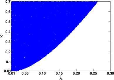
The scalar mass-squared matrices (both CP odd and CP even) and the vacuum expectation values νicsubscriptsuperscript𝜈𝑐𝑖\nu^{c}_{i} are not very sensitive to the change in neutrino Yukawa couplings (Yνsubscript𝑌𝜈Y_{\nu} 𝒪similar-toabsent𝒪\sim\cal{O} (107)superscript107(10^{-7})) and the corresponding soft parameter AνYνsubscript𝐴𝜈subscript𝑌𝜈A_{\nu}Y_{\nu} (𝒪similar-toabsent𝒪\sim\cal{O} (104)superscript104(10^{-4}) GeV). On the other hand, the values of tanβ𝛽\tan\beta and the coefficients λ𝜆\lambda and κ𝜅\kappa are very important in order to satisfy various constraints on the scalar sector mentioned earlier. In fig.1, we have plotted the allowed regions in the (λ𝜆\lambdaκ𝜅\kappa) plane for tanβ=10𝛽10\tan\beta=10.

Refer to caption
Figure 1: Allowed regions in (λ𝜆\lambdaκ𝜅\kappa) plane which satisfy various constraints on the scalar sector, for tanβ=10𝛽10\beta=10. λ𝜆\lambda and κ𝜅\kappa were allowed to vary from 0.005 to 0.50 and 0.005 to 0.70, respectively.

The values of other parameters are chosen to be mL~=400GeVsubscript𝑚~𝐿400GeVm_{\tilde{L}}=400~{}{\text{GeV}}, mν~c=300GeV,subscript𝑚superscript~𝜈𝑐300GeVm_{\tilde{\nu}^{c}}=300~{}{\text{GeV}}, Yν11=5.0×10⁷superscriptsubscript𝑌𝜈115.0superscript107Y_{\nu}^{11}=5.0\times 10^{-7}, Yν22=4.0×10⁷superscriptsubscript𝑌𝜈224.0superscript107Y_{\nu}^{22}=4.0\times 10^{-7}, Yν33=3.0×10⁷superscriptsubscript𝑌𝜈333.0superscript107Y_{\nu}^{33}=3.0\times 10^{-7}, (AνYν)ij=1TeV×Yνijsuperscriptsubscript𝐴𝜈subscript𝑌𝜈𝑖𝑗1TeVsuperscriptsubscript𝑌𝜈𝑖𝑗(A_{\nu}Y_{\nu})^{ij}=1~{}{\rm TeV}\times Y_{\nu}^{ij}, (Aλλ)=1TeV×λsubscript𝐴𝜆𝜆1TeV𝜆(A_{\lambda}\lambda)=-1~{}{\rm TeV}\times\lambda, and (Aκκ)=1TeV×κsubscript𝐴𝜅𝜅1TeV𝜅(A_{\kappa}\kappa)=1~{}{\rm TeV}\times\kappa. The upper limit of the value of κ𝜅\kappa is taken to be similar-to\sim 0.7 because of the constraints coming from the existence of Landau pole [9]. With these values of different parameters satisfying the constraints in the scalar sector, we will go on to calculate the neutrino masses and the mixing patterns as well as the decays of the lightest neutralino in this model as discussed in the next few sections.

It should be mentioned at this point that the radiative corrections to the light Higgs mass, can be significant in some regions of the parameter space as discussed in ref.[9]. It has been shown that the light Higgs mass larger than the LEP lower limit of 114 GeV can be obtained with the value of Atsubscript𝐴𝑡A_{t} (trilinear coupling in the scalar sector for the stop) within 1-2.4 TeV and when the mixing of the light Higgs with the right-handed sneutrino is small. The latter requirement is fulfilled in most of the cases that we have considered and in some cases the mixing is slightly larger. However, there is always the freedom of choosing the value of Atsubscript𝐴𝑡A_{t} appropriately. Hence, it would be fair to say that the experimental limits on the light Higgs boson mass can be satisfied in our analysis. The parameter points we have chosen here are sample points with different dominant composition of the lightest neutralino. Since we have a large parameter space, it is always possible to choose a different parameter point with the same characteristic features satisfying all the experimental constraints.

4 The fermionic sector

4.1 The neutral fermions

In this model, because of the breaking of R-parity, two neutral gauginos, B~0(=iλ~1)annotatedsuperscript~𝐵0absent𝑖subscript~𝜆1\tilde{B}^{0}(=-i{\tilde{\lambda}}_{1}) and W~30(=iλ~23)annotatedsuperscriptsubscript~𝑊30absent𝑖superscriptsubscript~𝜆23\tilde{W}_{3}^{0}(=-i{\tilde{\lambda}}_{2}^{3}) and two neutral higgsinos (H~10superscriptsubscript~𝐻10{\tilde{H}}_{1}^{0} and H~20superscriptsubscript~𝐻20{\tilde{H}}_{2}^{0}) are now mixed with the neutrinos (both νisubscript𝜈𝑖\nu_{i} and νicsuperscriptsubscript𝜈𝑖𝑐\nu_{i}^{c}). As can be seen from the superpotential (fourth and fifth term in eq. (4)4(\ref{superpotential})), the fermionic partners of ν~icsubscriptsuperscript~𝜈𝑐𝑖{\tilde{\nu}}^{c}_{i} and νi~~subscript𝜈𝑖\tilde{\nu_{i}} mix with the neutral higgsinos [8, 9]. The neutral gauginos are mixed with the left-handed neutrinos through the vacuum expectation values of the doublet sneutrinos. Mass matrices for the neutral and charged fermion sectors, involving all three generations of neutrinos (both doublet and singlet) and charged leptons, have been addressed also in [9].

In the weak interaction basis defined by

Ψ0T=(B~0,W~30,H~10,H~20,νec,νμc,ντc,νe,νμ,ντ),superscriptsuperscriptΨ0𝑇superscript~𝐵0superscriptsubscript~𝑊30superscriptsubscript~𝐻10superscriptsubscript~𝐻20subscriptsuperscript𝜈𝑐𝑒subscriptsuperscript𝜈𝑐𝜇subscriptsuperscript𝜈𝑐𝜏subscript𝜈𝑒subscript𝜈𝜇subscript𝜈𝜏\displaystyle{\Psi^{0}}^{T}=\left(\tilde{B}^{0},\tilde{W}_{3}^{0},\tilde{H}_{1}^{0},\tilde{H}_{2}^{0},{\nu^{c}_{e}},{\nu^{c}_{\mu}},{\nu^{c}_{\tau}},{\nu_{e}},{\nu_{\mu}},{\nu_{\tau}}\right), (14)

the neutral fermion mass term in the Lagrangian is of the form

neutralmass=12Ψ0TnΨ0+H.c.,superscriptsubscript𝑛𝑒𝑢𝑡𝑟𝑎𝑙𝑚𝑎𝑠𝑠12superscriptsuperscriptΨ0𝑇subscript𝑛superscriptΨ0H.c.\displaystyle{\mathcal{L}_{neutral}^{mass}}=-\frac{1}{2}{{\Psi^{0}}^{T}}\mathcal{M}_{n}{\Psi^{0}}+\text{H.c.}, (15)

where nsubscript𝑛\mathcal{M}_{n} includes all three generations of doublet and gauge singlet neutrinos and thus it is a 10×10101010\times 10 matrix. The massless neutrinos become massive due to this mixing with the neutralinos and the gauge singlet neutrinos. The three lightest eigenvalues of this 10×10101010\times 10 neutralino mass matrix correspond to the three light physical neutrinos and their masses have to be very small in order to satisfy the experimental data on massive neutrinos. The matrix nsubscript𝑛\mathcal{M}_{n} can be written in the following manner

n=(M7×7m3×7Tm3×703×3),subscript𝑛subscript𝑀77superscriptsubscript𝑚37𝑇subscript𝑚37subscript033\mathcal{M}_{n}=\left(\begin{array}[]{cc}M_{7\times 7}&m_{3\times 7}^{T}\\ m_{3\times 7}&0_{3\times 3}\end{array}\right), (16)

where

M7×7=(M10g12v1g12v20000M2g22v1g22v2000g12v1g22v10μλev2λμv2λτv2g12v2g22v2μ0ρeρμρτ00λev2ρe2ucee2uceμ2uceτ00λμv2ρμ2ucμe2ucμμ2ucμτ00λτv2ρτ2ucτe2ucτμ2ucττ),subscript𝑀77subscript𝑀10subscript𝑔12subscript𝑣1subscript𝑔12subscript𝑣2000missing-subexpressionmissing-subexpressionmissing-subexpressionmissing-subexpressionmissing-subexpressionmissing-subexpressionmissing-subexpression0subscript𝑀2subscript𝑔22subscript𝑣1subscript𝑔22subscript𝑣2000missing-subexpressionmissing-subexpressionmissing-subexpressionmissing-subexpressionmissing-subexpressionmissing-subexpressionmissing-subexpressionsubscript𝑔12subscript𝑣1subscript𝑔22subscript𝑣10𝜇superscript𝜆𝑒subscript𝑣2superscript𝜆𝜇subscript𝑣2superscript𝜆𝜏subscript𝑣2missing-subexpressionmissing-subexpressionmissing-subexpressionmissing-subexpressionmissing-subexpressionmissing-subexpressionmissing-subexpressionsubscript𝑔12subscript𝑣2subscript𝑔22subscript𝑣2𝜇0superscript𝜌𝑒superscript𝜌𝜇superscript𝜌𝜏missing-subexpressionmissing-subexpressionmissing-subexpressionmissing-subexpressionmissing-subexpressionmissing-subexpressionmissing-subexpression00superscript𝜆𝑒subscript𝑣2superscript𝜌𝑒2subscriptsuperscript𝑢𝑒𝑒𝑐2subscriptsuperscript𝑢𝑒𝜇𝑐2subscriptsuperscript𝑢𝑒𝜏𝑐missing-subexpressionmissing-subexpressionmissing-subexpressionmissing-subexpressionmissing-subexpressionmissing-subexpressionmissing-subexpression00superscript𝜆𝜇subscript𝑣2superscript𝜌𝜇2subscriptsuperscript𝑢𝜇𝑒𝑐2subscriptsuperscript𝑢𝜇𝜇𝑐2subscriptsuperscript𝑢𝜇𝜏𝑐missing-subexpressionmissing-subexpressionmissing-subexpressionmissing-subexpressionmissing-subexpressionmissing-subexpressionmissing-subexpression00superscript𝜆𝜏subscript𝑣2superscript𝜌𝜏2subscriptsuperscript𝑢𝜏𝑒𝑐2subscriptsuperscript𝑢𝜏𝜇𝑐2subscriptsuperscript𝑢𝜏𝜏𝑐M_{7\times 7}=\left(\begin{array}[]{ccccccc}M_{1}&0&-\frac{g_{1}}{\sqrt{2}}v_{1}&\frac{g_{1}}{\sqrt{2}}v_{2}&0&0&0\\ \\ 0&M_{2}&\frac{g_{2}}{\sqrt{2}}v_{1}&-\frac{g_{2}}{\sqrt{2}}v_{2}&0&0&0\\ \\ -\frac{g_{1}}{\sqrt{2}}v_{1}&\frac{g_{2}}{\sqrt{2}}v_{1}&0&-{\mu}&-{\lambda^{e}}v_{2}&-{\lambda^{\mu}}v_{2}&-{\lambda^{\tau}}v_{2}\\ \\ \frac{g_{1}}{\sqrt{2}}v_{2}&-\frac{g_{2}}{\sqrt{2}}v_{2}&-{\mu}&0&{\rho^{e}}&{\rho^{\mu}}&{\rho^{\tau}}\\ \\ 0&0&-{\lambda^{e}}v_{2}&{\rho^{e}}&2{u^{ee}_{c}}&2{u^{e{\mu}}_{c}}&2{u^{e{\tau}}_{c}}\\ \\ 0&0&-{\lambda^{\mu}}v_{2}&{\rho^{\mu}}&2{u^{{\mu}e}_{c}}&2{u^{{\mu}{\mu}}_{c}}&2{u^{{\mu}{\tau}}_{c}}\\ \\ 0&0&-{\lambda^{\tau}}v_{2}&{\rho^{\tau}}&2{u^{{\tau}e}_{c}}&2{u^{{\tau}{\mu}}_{c}}&2{u^{{\tau}{\tau}}_{c}}\end{array}\right), (17)

and

m3×7=(g12νeg22νe0rceYνeev2Yνeμv2Yνeτv2g12νμg22νμ0rcμYνμev2Yνμμv2Yνμτv2g12ντg22ντ0rcτYντev2Yντμv2Yνττv2).subscript𝑚37subscript𝑔12subscript𝜈𝑒subscript𝑔22subscript𝜈𝑒0subscriptsuperscript𝑟𝑒𝑐superscriptsubscript𝑌𝜈𝑒𝑒subscript𝑣2superscriptsubscript𝑌𝜈𝑒𝜇subscript𝑣2superscriptsubscript𝑌𝜈𝑒𝜏subscript𝑣2missing-subexpressionmissing-subexpressionmissing-subexpressionmissing-subexpressionmissing-subexpressionmissing-subexpressionmissing-subexpressionsubscript𝑔12subscript𝜈𝜇subscript𝑔22subscript𝜈𝜇0subscriptsuperscript𝑟𝜇𝑐superscriptsubscript𝑌𝜈𝜇𝑒subscript𝑣2superscriptsubscript𝑌𝜈𝜇𝜇subscript𝑣2superscriptsubscript𝑌𝜈𝜇𝜏subscript𝑣2missing-subexpressionmissing-subexpressionmissing-subexpressionmissing-subexpressionmissing-subexpressionmissing-subexpressionmissing-subexpressionsubscript𝑔12subscript𝜈𝜏subscript𝑔22subscript𝜈𝜏0subscriptsuperscript𝑟𝜏𝑐superscriptsubscript𝑌𝜈𝜏𝑒subscript𝑣2superscriptsubscript𝑌𝜈𝜏𝜇subscript𝑣2superscriptsubscript𝑌𝜈𝜏𝜏subscript𝑣2m_{3\times 7}=\left(\begin{array}[]{ccccccc}-\frac{g_{1}}{\sqrt{2}}{\nu_{e}}&\frac{g_{2}}{\sqrt{2}}{\nu_{e}}&0&{r^{e}_{c}}&Y_{\nu}^{ee}v_{2}&Y_{\nu}^{e{\mu}}v_{2}&Y_{\nu}^{e{\tau}}v_{2}\\ \\ -\frac{g_{1}}{\sqrt{2}}{\nu_{\mu}}&\frac{g_{2}}{\sqrt{2}}{\nu_{\mu}}&0&{r^{\mu}_{c}}&Y_{\nu}^{{\mu}e}v_{2}&Y_{\nu}^{{\mu}{\mu}}v_{2}&Y_{\nu}^{{\mu}{\tau}}v_{2}\\ \\ -\frac{g_{1}}{\sqrt{2}}{\nu_{\tau}}&\frac{g_{2}}{\sqrt{2}}{\nu_{\tau}}&0&{r^{\tau}_{c}}&Y_{\nu}^{{\tau}e}v_{2}&Y_{\nu}^{{\tau}{\mu}}v_{2}&Y_{\nu}^{{\tau}{\tau}}v_{2}\end{array}\right). (18)

Note that the top-left 4×4444\times 4 block of the matrix M7×7subscript𝑀77M_{7\times 7} is the usual neutralino mass matrix of the MSSM. The bottom right 3×3333\times 3 block is the Majorana mass matrix of gauge singlet neutrinos, which will be taken as diagonal in our subsequent analysis. The entries of M7×7subscript𝑀77M_{7\times 7} are in general of the order of the electroweak scale and the entries of m3×7subscript𝑚37m_{3\times 7} are much smaller (similar-to\sim 𝒪𝒪\cal O(105superscript10510^{-5} GeV)). Hence, the matrix (16) has a seesaw structure that will give rise to three very light eigenvalues corresponding to three light neutrinos. The correct neutrino mass scale of similar-to\sim 102superscript10210^{-2} eV can easily be obtained with such a structure of the 10×10101010\times 10 neutralino mass matrix. In this work our focus would be to see if one can obtain the correct mass-squared differences and the mixing pattern for the light neutrinos even if we consider flavour diagonal neutrino Yukawa couplings in eq.(18) (i.e. with a diagonal Dirac neutrino mass matrix). This makes the analysis simpler with a reduced number of parameters and makes the model more predictive. As we will show later, it is possible to find out the correct mixing pattern and the mass hierarchies (both normal and inverted) among the light neutrinos in such a situation, at the tree level.

In order to obtain the physical neutralino states, one needs to diagonalize the 10×10101010\times 10 matrix nsubscript𝑛\mathcal{M}_{n}. As in the case of MSSM, the symmetric mass matrix nsubscript𝑛\mathcal{M}_{n} can be diagonalized with one unitary matrix N𝑁N. The mass eigenstates are defined by

χ~i0=NijΨj0,i,j=1,,10,formulae-sequencesubscriptsuperscript~𝜒0𝑖subscript𝑁𝑖𝑗subscriptsuperscriptΨ0𝑗𝑖𝑗110{\tilde{\chi}}^{0}_{i}=N_{ij}\Psi^{0}_{j},\quad i,j=1,...,10, (19)

where the 10×10101010\times 10 unitary matrix N𝑁N satisfies

NnN1=D0,superscript𝑁subscript𝑛superscript𝑁1subscriptsuperscript0𝐷N^{*}\mathcal{M}_{n}N^{-1}=\mathcal{M}^{0}_{D}, (20)

with the diagonal neutralino mass matrix denoted as D0subscriptsuperscript0𝐷\mathcal{M}^{0}_{D}. The matrix N𝑁N may be chosen in such a way that elements of D0subscriptsuperscript0𝐷\mathcal{M}^{0}_{D} are real and non-negative. In our analysis we will assume that all the entries in the 10×10101010\times 10 neutralino mass matrix Mnsubscript𝑀𝑛M_{n} are real. Seven eigenstates of this matrix are heavy, i.e. of the order of the electroweak scale. Out of these seven states, there are four states which are usually very similar to the MSSM neutralinos. The remaining three states are mostly dominated by νicsubscriptsuperscript𝜈𝑐𝑖\nu^{c}_{i}. It is, in general, very difficult to predict the nature of the lightest of these seven states since that depends on several unknown parameters. In our analysis of the decays of the lightest supersymmetric particle (LSP), we will concentrate on three different possibilities::\colon (i) lightest state is dominated by the bino component, (ii) higgsino dominated lightest state, and (iii) gauge singlet neutrinos νicsubscriptsuperscript𝜈𝑐𝑖\nu^{c}_{i} form the lightest state. The last possibility is very interesting since in this case we have the opportunity to produce the gauge singlet neutrinos at the LHC and study their properties through the R-parity violating decay modes. This way one has a direct probe to the seesaw scale at the LHC.

4.2 The charged fermions

In the charged fermion sector, the charged gauginos and charged higgsinos mix with the charged leptons because of the presence of the effective bilinear RPV parameters ϵijYνijνjcsuperscriptitalic-ϵ𝑖subscript𝑗subscriptsuperscript𝑌𝑖𝑗𝜈subscriptsuperscript𝜈𝑐𝑗\epsilon^{i}\equiv\sum_{j}Y^{ij}_{\nu}\nu^{c}_{j} and the sneutrino VEVs νisubscript𝜈𝑖\nu_{i}. This is similar to the case of MSSM with bilinear RPV with the parameter μ𝜇\mu defined as μ=iλiνic𝜇subscript𝑖superscript𝜆𝑖subscriptsuperscript𝜈𝑐𝑖\mu=\sum_{i}\lambda^{i}\nu^{c}_{i}. Since we want to calculate the decays of the lightest neutralino, we also need to know the mass eigenvalues and the mixing matrices in the charged fermion sector. Because of this reason, we discuss the chargino mass matrix in some details. In the weak interaction basis defined by

Ψ+T=(iλ~2+,H~2+,eR+,μR+,τR+),superscriptΨ𝑇𝑖subscriptsuperscript~𝜆2superscriptsubscript~𝐻2superscriptsubscript𝑒𝑅superscriptsubscript𝜇𝑅superscriptsubscript𝜏𝑅\displaystyle{\Psi^{+T}}=(-i\tilde{\lambda}^{+}_{2},\tilde{H}_{2}^{+},e_{R}^{+},\mu_{R}^{+},\tau_{R}^{+}),
ΨT=(iλ~2,H~1,eL,μL,τL).superscriptΨ𝑇𝑖superscriptsubscript~𝜆2superscriptsubscript~𝐻1superscriptsubscript𝑒𝐿superscriptsubscript𝜇𝐿superscriptsubscript𝜏𝐿\displaystyle{\Psi^{-T}}=(-i\tilde{\lambda}_{2}^{-},\tilde{H}_{1}^{-},e_{L}^{-},\mu_{L}^{-},\tau_{L}^{-}).
(21)

The charged fermion mass term in the Lagrangian is of the form

chargedmass=12(Ψ+TΨT)(05×5m5×5Tm5×505×5)(Ψ+Ψ).superscriptsubscript𝑐𝑎𝑟𝑔𝑒𝑑𝑚𝑎𝑠𝑠12superscriptΨsuperscript𝑇superscriptΨsuperscript𝑇subscript055superscriptsubscript𝑚55𝑇missing-subexpressionmissing-subexpressionsubscript𝑚55subscript055superscriptΨmissing-subexpressionsuperscriptΨ{\mathcal{L}_{charged}^{mass}}=-\frac{1}{2}\left(\begin{array}[]{cc}\Psi^{+^{T}}&\Psi^{-^{T}}\end{array}\right)\left(\begin{array}[]{cc}0_{5\times 5}&m_{5\times 5}^{T}\\ \\ m_{5\times 5}&0_{5\times 5}\end{array}\right)\left(\begin{array}[]{c}\Psi^{+}\\ \\ \Psi^{-}\end{array}\right). (22)

Here we have included all three generations of charged leptons and assumed that the charged lepton Yukawa couplings are in the diagonal form. Also, iλ±𝑖superscript𝜆plus-or-minus-i\lambda^{\pm} are the two-component charged Wino fields and H~1superscriptsubscript~𝐻1{\tilde{H}}_{1}^{-} and H~2+superscriptsubscript~𝐻2{\tilde{H}}_{2}^{+} are the two-component charged higgsino fields. The matrix m5×5subscript𝑚55m_{5\times 5} is given by

m5×5=(M2g2v2000g2v1μYeeeνeYeμμνμYeττντg2νerceYeeev100g2νμrcμ0Yeμμv10g2ντrcτ00Yeττv1).subscript𝑚55subscript𝑀2subscript𝑔2subscript𝑣2000missing-subexpressionmissing-subexpressionmissing-subexpressionmissing-subexpressionmissing-subexpressionsubscript𝑔2subscript𝑣1𝜇superscriptsubscript𝑌𝑒𝑒𝑒subscript𝜈𝑒superscriptsubscript𝑌𝑒𝜇𝜇subscript𝜈𝜇superscriptsubscript𝑌𝑒𝜏𝜏subscript𝜈𝜏missing-subexpressionmissing-subexpressionmissing-subexpressionmissing-subexpressionmissing-subexpressionsubscript𝑔2subscript𝜈𝑒subscriptsuperscript𝑟𝑒𝑐superscriptsubscript𝑌𝑒𝑒𝑒subscript𝑣100missing-subexpressionmissing-subexpressionmissing-subexpressionmissing-subexpressionmissing-subexpressionsubscript𝑔2subscript𝜈𝜇subscriptsuperscript𝑟𝜇𝑐0superscriptsubscript𝑌𝑒𝜇𝜇subscript𝑣10missing-subexpressionmissing-subexpressionmissing-subexpressionmissing-subexpressionmissing-subexpressionsubscript𝑔2subscript𝜈𝜏subscriptsuperscript𝑟𝜏𝑐00superscriptsubscript𝑌𝑒𝜏𝜏subscript𝑣1m_{5\times 5}=\left(\begin{array}[]{ccccc}M_{2}&{g_{2}}{v_{2}}&0&0&0\\ \\ {g_{2}}{v_{1}}&{\mu}&-{Y_{e}^{ee}}{\nu_{e}}&-{Y_{e}^{{\mu}{\mu}}}{\nu_{\mu}}&-{Y_{e}^{{\tau}{\tau}}}{\nu_{\tau}}\\ \\ {g_{2}}{\nu_{e}}&-{r^{e}_{c}}&{Y_{e}^{ee}}{v_{1}}&0&0\\ \\ {g_{2}}{\nu_{\mu}}&-{r^{\mu}_{c}}&0&{Y_{e}^{{\mu}{\mu}}}{v_{1}}&0\\ \\ {g_{2}}{\nu_{\tau}}&-{r^{\tau}_{c}}&0&0&{Y_{e}^{{\tau}{\tau}}}{v_{1}}\end{array}\right). (23)

The charged fermion masses are obtained by applying a bi-unitary transformation such that

Um5×5V1=D±,superscript𝑈subscript𝑚55superscript𝑉1subscriptsuperscriptplus-or-minus𝐷U^{*}m_{5\times 5}V^{-1}=\mathcal{M}^{\pm}_{D}, (24)

where Usuperscript𝑈U^{*} and V𝑉V are two unitary matrices and D±subscriptsuperscriptplus-or-minus𝐷\mathcal{M}^{\pm}_{D} is the diagonal matrix with non-negative entries corresponding to the physical fermion masses. The two-component mass eigenstates are defined by

χi+=VijΨj+,subscriptsuperscript𝜒𝑖subscript𝑉𝑖𝑗subscriptsuperscriptΨ𝑗\displaystyle\chi^{+}_{i}=V_{ij}\Psi^{+}_{j},
χi=UijΨj,i,j=1,,5.formulae-sequencesubscriptsuperscript𝜒𝑖subscript𝑈𝑖𝑗subscriptsuperscriptΨ𝑗𝑖𝑗15\displaystyle\chi^{-}_{i}=U_{ij}\Psi^{-}_{j},\quad i,j=1,...,5. (25)

Nevertheless, we notice that the 13, 14, and 15 elements of the chargino mass matrix (eq. (23)) are vanishing and given the orders of magnitude of various parameters, we also see that the values of the other off-diagonal entries (except for 12 and 21 elements) are very small. This indicates that the physical charged lepton eigenstates will have a very small admixture of charged higgsino and charged gaugino states. So we can very well assume (also verified numerically) that this mixing has very little effect on the mass eigenstates of the charged leptons. Thus, while writing down the neutrino mixing matrix, it will be justified to assume that one is working in the basis where the charged lepton mass matrix is already in the diagonal form.

5 Neutrinos

5.1 Seesaw masses

When lepton-number violation is allowed, the effective light neutrino mass matrix arising via the seesaw mechanism is in general given by

Mν=m3×7M7×71m3×7T.superscript𝑀𝜈subscript𝑚37superscriptsubscript𝑀771superscriptsubscript𝑚37𝑇{M^{\nu}}=-{m_{3\times 7}}{M_{7\times 7}^{-1}}{m_{3\times 7}^{T}}. (26)

As discussed in the previous section, m3×7subscript𝑚37{m_{3\times 7}} is the so-called Dirac neutrino mass matrix and M7×7subscript𝑀77{M_{7\times 7}} is the matrix for the heavy states and contains ΔL=2Δ𝐿2\Delta{L}=2 mass terms for right chiral neutrinos. In order to find out the neutrino mass-squared differences and mixing angles, one must diagonalize the matrix Mνsuperscript𝑀𝜈M^{\nu} to find out the eigenvalues and the eigenvectors. Before discussing the detailed numerical results, let us try to understand the characteristic features of this neutrino mass matrix analytically. Let us note that the neutrino mass-squared differences indicate three possible scenarios for the light neutrino mass spectrum. They are (i) Normal hierarchy corresponding to m1m2Δm212subscript𝑚1subscript𝑚2similar-toΔsubscriptsuperscript𝑚221m_{1}\approx m_{2}\sim\sqrt{\Delta m^{2}_{21}}m3|Δm312|similar-tosubscript𝑚3Δsubscriptsuperscript𝑚231m_{3}\sim\sqrt{|\Delta m^{2}_{31}|}, (ii) Inverted hierarchy::\colon m1m2|Δm312|subscript𝑚1subscript𝑚2similar-toΔsubscriptsuperscript𝑚231m_{1}\approx m_{2}\sim\sqrt{|\Delta m^{2}_{31}|}, m3|Δm312|much-less-thansubscript𝑚3Δsubscriptsuperscript𝑚231m_{3}\ll\sqrt{|\Delta m^{2}_{31}|} and (iii) Degenerate masses::\colon m1m2m3|Δm312|subscript𝑚1subscript𝑚2subscript𝑚3much-greater-thanΔsubscriptsuperscript𝑚231m_{1}\approx m_{2}\approx m_{3}\gg\sqrt{|\Delta m^{2}_{31}|}, where m1subscript𝑚1m_{1}, m2subscript𝑚2m_{2}, and m3subscript𝑚3m_{3} are the three light neutrino mass eigenvalues.

5.1.1 Analytical results

Let us make a few simplifications in order to diagonalize the effective light neutrino mass matrix. One should note that the neutrino mass matrix involves the vacuum expectation values for the doublet and the gauge singlet sneutrinos. Hence we also make some simplifying assumptions for the parameters appearing in the scalar sector. Some of these assumptions have already been mentioned in the scalar sector but here we repeat them for the convenience of the reader. We have defined

κijk=κ,ifi=j=k,and zero otherwise,formulae-sequenceformulae-sequencesuperscript𝜅𝑖𝑗𝑘𝜅if𝑖𝑗𝑘and zero otherwise\displaystyle{\kappa^{ijk}}={\kappa},{\hskip 5.69046pt}\text{if}{\hskip 5.69046pt}{i=j=k},{\hskip 5.69046pt}\text{and zero otherwise},
(Aκκ)ijk=(Aκκ),ifi=j=k,and zero otherwise,formulae-sequenceformulae-sequencesuperscriptsubscript𝐴𝜅𝜅𝑖𝑗𝑘subscript𝐴𝜅𝜅if𝑖𝑗𝑘and zero otherwise\displaystyle{(A_{\kappa}\kappa)^{ijk}}=(A_{\kappa}\kappa),{\hskip 5.69046pt}\text{if}{\hskip 5.69046pt}{i=j=k},{\hskip 5.69046pt}\text{and zero otherwise},
Yνij=0,ifij,formulae-sequencesuperscriptsubscript𝑌𝜈𝑖𝑗0if𝑖𝑗\displaystyle{Y_{\nu}^{ij}}=0,\hskip 5.69046pt\text{if}\hskip 5.69046pt{i\neq j},
(AνYν)ij=0,ifij,formulae-sequencesuperscriptsubscript𝐴𝜈subscript𝑌𝜈𝑖𝑗0if𝑖𝑗\displaystyle(A_{\nu}Y_{\nu})^{ij}=0,\hskip 5.69046pt\text{if}\hskip 5.69046pt{i\neq j},
λ1=λ2=λ3=λ,superscript𝜆1superscript𝜆2superscript𝜆3𝜆\displaystyle{\lambda^{1}}={\lambda^{2}}={\lambda^{3}}={\lambda},
(Aλλ)1=(Aλλ)2=(Aλλ)3=(Aλλ),superscriptsubscript𝐴𝜆𝜆1superscriptsubscript𝐴𝜆𝜆2superscriptsubscript𝐴𝜆𝜆3subscript𝐴𝜆𝜆\displaystyle{(A_{\lambda}\lambda)^{1}}={(A_{\lambda}\lambda)^{2}}={(A_{\lambda}\lambda)^{3}}={(A_{\lambda}\lambda)},
(mL~2)ij=(mL~2)δij,superscriptsubscriptsuperscript𝑚2~𝐿𝑖𝑗subscriptsuperscript𝑚2~𝐿superscript𝛿𝑖𝑗\displaystyle(m^{2}_{\tilde{L}})^{ij}=(m^{2}_{\tilde{L}})\delta^{ij},
(mν~c2)ij=(mν~c2)δij,superscriptsubscriptsuperscript𝑚2superscript~𝜈𝑐𝑖𝑗subscriptsuperscript𝑚2superscript~𝜈𝑐superscript𝛿𝑖𝑗\displaystyle(m^{2}_{\tilde{\nu}^{c}})^{ij}=(m^{2}_{\tilde{\nu}^{c}})\delta^{ij}, (27)

where i,j,k=e,μ,τformulae-sequence𝑖𝑗𝑘𝑒𝜇𝜏i,j,k=e,\mu,\tau in the flavour basis.

With these assumptions one can solve for νicsubscriptsuperscript𝜈𝑐𝑖\nu^{c}_{i} from the minimization equations for the gauge singlet sneutrinos (eq.(8)) and the result is ν1c=ν2c=ν3c=νcsubscriptsuperscript𝜈𝑐1subscriptsuperscript𝜈𝑐2subscriptsuperscript𝜈𝑐3superscript𝜈𝑐{\nu^{c}_{1}}={\nu^{c}_{2}}={\nu^{c}_{3}}={\nu^{c}}. This can be understood if we neglect the terms proportional to Yν2superscriptsubscript𝑌𝜈2{Y_{\nu}}^{2}, Yννsubscript𝑌𝜈𝜈{Y_{\nu}}{\nu}, (AνYν)νsubscript𝐴𝜈subscript𝑌𝜈𝜈({A_{\nu}}{Y_{\nu}}){\nu} in the minimization equations and assume that λ,κ𝜆𝜅\lambda,\kappa are 𝒪similar-toabsent𝒪\sim{\cal O}(1) couplings.

Now let us look at the effective left chiral neutrino mass matrix (eq.(26)) in a little more details. Because of the smallness of Yνsubscript𝑌𝜈Y_{\nu} and νisubscript𝜈𝑖\nu_{i}, one can neglect terms containing Yν2ν2superscriptsubscript𝑌𝜈2superscript𝜈2{Y_{\nu}}^{2}{\nu^{2}} and Yν3νsuperscriptsubscript𝑌𝜈3𝜈{Y_{\nu}}^{3}{\nu}. This way one obtains an approximate analytical expression for the 3×3333\times 3 neutrino mass matrix.

Mν=23AνcΔ(be2bebμbebτbebμbμ2bμbτbebτbμbτbτ2)+16κνc(2ae2aeaμaeaτaeaμ2aμ2aμaτaeaτaμaτ2aτ2)superscript𝑀𝜈23𝐴superscript𝜈𝑐Δsubscriptsuperscript𝑏2𝑒subscript𝑏𝑒subscript𝑏𝜇subscript𝑏𝑒subscript𝑏𝜏missing-subexpressionmissing-subexpressionmissing-subexpressionsubscript𝑏𝑒subscript𝑏𝜇subscriptsuperscript𝑏2𝜇subscript𝑏𝜇subscript𝑏𝜏missing-subexpressionmissing-subexpressionmissing-subexpressionsubscript𝑏𝑒subscript𝑏𝜏subscript𝑏𝜇subscript𝑏𝜏subscriptsuperscript𝑏2𝜏16𝜅superscript𝜈𝑐2subscriptsuperscript𝑎2𝑒subscript𝑎𝑒subscript𝑎𝜇subscript𝑎𝑒subscript𝑎𝜏missing-subexpressionmissing-subexpressionmissing-subexpressionsubscript𝑎𝑒subscript𝑎𝜇2subscriptsuperscript𝑎2𝜇subscript𝑎𝜇subscript𝑎𝜏missing-subexpressionmissing-subexpressionmissing-subexpressionsubscript𝑎𝑒subscript𝑎𝜏subscript𝑎𝜇subscript𝑎𝜏2subscriptsuperscript𝑎2𝜏\displaystyle{M^{\nu}}={\frac{2}{3}}{\frac{A{\nu^{c}}}{\Delta}}\left(\begin{array}[]{ccc}b^{2}_{e}&b_{e}b_{\mu}&b_{e}b_{\tau}\\ \\ b_{e}b_{\mu}&b^{2}_{\mu}&b_{\mu}b_{\tau}\\ \\ b_{e}b_{\tau}&b_{\mu}b_{\tau}&b^{2}_{\tau}\end{array}\right)+{{\frac{1}{6{\kappa}{\nu^{c}}}}}\left(\begin{array}[]{ccc}-2a^{2}_{e}&a_{e}a_{\mu}&a_{e}a_{\tau}\\ \\ a_{e}a_{\mu}&-2a^{2}_{\mu}&a_{\mu}a_{\tau}\\ \\ a_{e}a_{\tau}&a_{\mu}a_{\tau}&-2a^{2}_{\tau}\end{array}\right) (38)
2λμ3ΔiYνiiνi(v22λABΔ)(ce2cecμcecτcecμcμ2cμcτcecτcμcτcτ2),2𝜆𝜇3Δsubscript𝑖superscriptsubscript𝑌𝜈𝑖𝑖subscript𝜈𝑖subscript𝑣22𝜆𝐴𝐵Δsubscriptsuperscript𝑐2𝑒subscript𝑐𝑒subscript𝑐𝜇subscript𝑐𝑒subscript𝑐𝜏missing-subexpressionmissing-subexpressionmissing-subexpressionsubscript𝑐𝑒subscript𝑐𝜇subscriptsuperscript𝑐2𝜇subscript𝑐𝜇subscript𝑐𝜏missing-subexpressionmissing-subexpressionmissing-subexpressionsubscript𝑐𝑒subscript𝑐𝜏subscript𝑐𝜇subscript𝑐𝜏subscriptsuperscript𝑐2𝜏\displaystyle-{\frac{2{\lambda}{\mu}}{3\Delta}}{\sum_{i}}Y_{\nu}^{ii}{\nu_{i}}\left(v_{2}-{\frac{{2\lambda}AB}{\Delta}}\right)\left(\begin{array}[]{ccc}c^{2}_{e}&c_{e}c_{\mu}&c_{e}c_{\tau}\\ \\ c_{e}c_{\mu}&c^{2}_{\mu}&c_{\mu}c_{\tau}\\ \\ c_{e}c_{\tau}&c_{\mu}c_{\tau}&c^{2}_{\tau}\end{array}\right), (44)
(45)

where

ΔΔ\displaystyle\Delta =\displaystyle= λ2(v12+v22)2+4λκνc2v1v24MλAμ,μ=3λνc,superscript𝜆2superscriptsubscriptsuperscript𝑣21subscriptsuperscript𝑣2224𝜆𝜅superscriptsuperscript𝜈𝑐2subscript𝑣1subscript𝑣24𝑀𝜆𝐴𝜇𝜇3𝜆superscript𝜈𝑐\displaystyle{\lambda}^{2}(v^{2}_{1}+v^{2}_{2})^{2}+4{\lambda}{\kappa}{\nu^{c}}^{2}v_{1}v_{2}-4M\lambda A{\mu},~{}\mu=3\lambda\nu^{c},
A𝐴\displaystyle A =\displaystyle= (κνc2+λv1v2),𝜅superscriptsuperscript𝜈𝑐2𝜆subscript𝑣1subscript𝑣2\displaystyle({\kappa}{\nu^{c}}^{2}+{\lambda}v_{1}v_{2}),
1M1𝑀\displaystyle\frac{1}{M} =\displaystyle= g12M1+g22M2,subscriptsuperscript𝑔21subscript𝑀1subscriptsuperscript𝑔22subscript𝑀2\displaystyle\frac{g^{2}_{1}}{M_{1}}+\frac{g^{2}_{2}}{M_{2}}, (46)
B𝐵\displaystyle B =\displaystyle= v1(v12+v22)2Mμv2,subscript𝑣1subscriptsuperscript𝑣21subscriptsuperscript𝑣222𝑀𝜇subscript𝑣2\displaystyle v_{1}(v^{2}_{1}+v^{2}_{2})-2M{\mu}v_{2},
aisubscript𝑎𝑖\displaystyle a_{i} =\displaystyle= Yνiiv2,bi=(Yνiiv1+3λνi),ci=νi,formulae-sequencesuperscriptsubscript𝑌𝜈𝑖𝑖subscript𝑣2subscript𝑏𝑖superscriptsubscript𝑌𝜈𝑖𝑖subscript𝑣13𝜆subscript𝜈𝑖subscript𝑐𝑖subscript𝜈𝑖\displaystyle Y_{\nu}^{ii}v_{2},~{}b_{i}=(Y_{\nu}^{ii}v_{1}+3{\lambda}{\nu_{i}}),~{}c_{i}={\nu_{i}},

with i,j,k=e,μ,τformulae-sequence𝑖𝑗𝑘𝑒𝜇𝜏{i,j,k}={e,\mu,\tau}.

One can rewrite eq. (45) in a compact form as follows

Mijν=2Aνc3Δbibj+16κνcaiaj(13δij)2λμ3ΔkYνkkνk(v22λABΔ)cicj.subscriptsuperscript𝑀𝜈𝑖𝑗2𝐴superscript𝜈𝑐3Δsubscript𝑏𝑖subscript𝑏𝑗16𝜅superscript𝜈𝑐subscript𝑎𝑖subscript𝑎𝑗13subscript𝛿𝑖𝑗2𝜆𝜇3Δsubscript𝑘superscriptsubscript𝑌𝜈𝑘𝑘subscript𝜈𝑘subscript𝑣22𝜆𝐴𝐵Δsubscript𝑐𝑖subscript𝑐𝑗M^{\nu}_{ij}={\frac{2A{\nu^{c}}}{3\Delta}}{b_{i}}{b_{j}}+{\frac{1}{6\kappa{\nu^{c}}}}{a_{i}}{a_{j}}(1-3\delta_{ij})-{\frac{2{\lambda}{\mu}}{3\Delta}}{\sum_{k}}Y_{\nu}^{kk}{\nu_{k}}\left(v_{2}-{\frac{{2\lambda}AB}{\Delta}}\right){c_{i}}{c_{j}}. (47)

Let us note that the smallness of the left chiral sneutrino VEVs (νi<<v1,v2much-less-thansubscript𝜈𝑖subscript𝑣1subscript𝑣2{\nu_{i}}<<v_{1},v_{2}) allows us to use mZ212(g12+g22)(v12+v22)subscriptsuperscript𝑚2𝑍12subscriptsuperscript𝑔21subscriptsuperscript𝑔22subscriptsuperscript𝑣21subscriptsuperscript𝑣22m^{2}_{Z}\approx{\frac{1}{2}}(g^{2}_{1}+g^{2}_{2})(v^{2}_{1}+v^{2}_{2}) and tanβv2v1𝛽subscript𝑣2subscript𝑣1\tan{\beta}\approx{\frac{v_{2}}{v_{1}}}.

The coefficients of the first term in eq.(45) (or in eq.(47)) is of the order of 1m~1~𝑚\frac{1}{\tilde{m}} whereas the coefficient of the second term is <fragmentsfragmentssimilar-to\mathrel{\mathchoice{\vbox{\offinterlineskip\halign{$\m@th\displaystyle\hfil#\hfil$\cr<\crcr\sim\crcr} }}{\vbox{\offinterlineskip\halign{$\m@th\textstyle\hfil#\hfil$\cr<\crcr\sim\crcr} }}{\vbox{\offinterlineskip\halign{$\m@th\scriptstyle\hfil#\hfil$\cr<\crcr\sim\crcr} }}{\vbox{\offinterlineskip\halign{$\m@th\scriptscriptstyle\hfil#\hfil$\cr<\crcr\sim\crcr} }}} 110m~110~𝑚\frac{1}{10{\tilde{m}}}, where m~~𝑚\tilde{m} is the electroweak (or supersymmetry breaking) scale and we have assumed that the relevant mass scales are at m~~𝑚\tilde{m} and κ𝜅\kappa is an order one coupling. The value of the coupling λ𝜆\lambda (determines the value of the μ𝜇\mu parameter), which satisfies the neutrino data as well as the constraints in the scalar sector, is taken to be of the order of 101superscript10110^{-1}. On the other hand, the coefficient of the third term is 1m~(νim~)similar-toabsent1~𝑚subscript𝜈𝑖~𝑚\sim\frac{1}{{\tilde{m}}}(\frac{\nu_{i}}{\tilde{m}}). Since νim~106similar-tosubscript𝜈𝑖~𝑚superscript106\frac{\nu_{i}}{\tilde{m}}\sim 10^{-6}107superscript10710^{-7}, there is an extra suppression factor in the elements of third term in eq.(45), compared to the first two terms. In addition, bi2ai2ci2similar-tosubscriptsuperscript𝑏2𝑖subscriptsuperscript𝑎2𝑖similar-tosubscriptsuperscript𝑐2𝑖b^{2}_{i}\sim a^{2}_{i}\sim c^{2}_{i} with a slightly larger value of ai2subscriptsuperscript𝑎2𝑖a^{2}_{i} and ci2subscriptsuperscript𝑐2𝑖c^{2}_{i} compared to bi2subscriptsuperscript𝑏2𝑖b^{2}_{i} in most cases. Hence, one can neglect the third term of eq.(45) in comparison to the first two terms. However, in our numerical analysis (discussed later) we have kept all the terms in eq.(45) and checked that the presence of the third term changes the result in an insignificant manner.

Before going on to find out the expressions for the eigenvalues and the eigenvectors of the effective neutrino mass matrix (eq.(45)), let us highlight a few limiting cases which give us some insight regarding the behaviour of the neutrino mass matrix. Neglecting the third term one can rewrite eq.(47) in the following manner

Mijνv226κνcYνiiYνjj(13δij)subscriptsuperscript𝑀𝜈𝑖𝑗subscriptsuperscript𝑣226𝜅superscript𝜈𝑐subscriptsuperscript𝑌𝑖𝑖𝜈subscriptsuperscript𝑌𝑗𝑗𝜈13𝛿𝑖𝑗\displaystyle M^{\nu}_{ij}\approx{\frac{v^{2}_{2}}{6\kappa{\nu^{c}}}}{Y^{ii}_{\nu}}{Y^{jj}_{\nu}}(1-3{\delta{ij}}) \displaystyle- 12M[νiνj+v1νc(Yνiiνj+Yνjjνi)μ+YνiiYνjjv12νc2μ2]12𝑀delimited-[]subscript𝜈𝑖subscript𝜈𝑗subscript𝑣1superscript𝜈𝑐subscriptsuperscript𝑌𝑖𝑖𝜈subscript𝜈𝑗subscriptsuperscript𝑌𝑗𝑗𝜈subscript𝜈𝑖𝜇subscriptsuperscript𝑌𝑖𝑖𝜈subscriptsuperscript𝑌𝑗𝑗𝜈subscriptsuperscript𝑣21superscriptsuperscript𝜈𝑐2superscript𝜇2\displaystyle{\frac{1}{2M}}\left[{\nu_{i}}{\nu_{j}}+{\frac{v_{1}{\nu^{c}}(Y^{ii}_{\nu}{\nu_{j}}+Y^{jj}_{\nu}{\nu_{i}})}{\mu}+{\frac{Y^{ii}_{\nu}Y^{jj}_{\nu}v^{2}_{1}{\nu^{c}}^{2}}{\mu^{2}}}}\right] (48)
×[1v22MAμ(κνc2sin2β+λv22)]1.absentsuperscriptdelimited-[]1superscript𝑣22𝑀𝐴𝜇𝜅superscriptsuperscript𝜈𝑐22𝛽𝜆superscript𝑣221\displaystyle{\times}\left[1-{\frac{v^{2}}{2MA{\mu}}}\left({\kappa}{\nu^{c}}^{2}\sin{2\beta}+{\frac{\lambda{v^{2}}}{2}}\right)\right]^{-1}.

Here we have used v2=vsinβ,v1=vcosβ,andμ=3λνcformulae-sequencesubscript𝑣2𝑣𝛽formulae-sequencesubscript𝑣1𝑣𝛽and𝜇3𝜆superscript𝜈𝑐v_{2}=v\sin{\beta},v_{1}=v\cos{\beta},\text{and}~{}\mu=3{\lambda}{\nu^{c}}.

In the limit νcsuperscript𝜈𝑐{\nu^{c}}\rightarrow\infty and v0𝑣0v\rightarrow 0, eq. (48) reduces to

Mijννiνj2M,subscriptsuperscript𝑀𝜈𝑖𝑗subscript𝜈𝑖subscript𝜈𝑗2𝑀M^{\nu}_{ij}\approx-{\frac{{\nu_{i}}{\nu_{j}}}{2M}}, (49)

which is the first part of the second term of eq.(48). In this case the elements of the neutrino mass matrix are bilinears in the left-handed sneutrino VEVs and they appear due to a seesaw effect involving the gauginos. This is called the “gaugino seesaw” effect and neutrino mass generation through this effect is a characteristic feature of the bilinear Rlimit-from𝑅R-parity violating model. This effect is present in this model because we have seen earlier that the effective bilinear R-parity violating terms are generated in the scalar potential as well as in the superpotential through the vacuum expectation values of the gauge singlet sneutrinos. Note that the gaugino seesaw effect can generate mass for only one doublet neutrino.

In the limit M𝑀M\rightarrow\infty, eq.(48) reduces to

Mijνv226κνcYνiiYνjj(13δij),subscriptsuperscript𝑀𝜈𝑖𝑗subscriptsuperscript𝑣226𝜅superscript𝜈𝑐subscriptsuperscript𝑌𝑖𝑖𝜈subscriptsuperscript𝑌𝑗𝑗𝜈13𝛿𝑖𝑗M^{\nu}_{ij}\approx{\frac{v^{2}_{2}}{6\kappa{\nu^{c}}}}{Y^{ii}_{\nu}}{Y^{jj}_{\nu}}(1-3{\delta{ij}}), (50)

which corresponds to the ordinary seesaw effect between the left handed and gauge singlet neutrinos. Remember that the effective Majorana masses for the gauge singlet neutrinos are given by MR=2κνcsubscript𝑀𝑅2𝜅superscript𝜈𝑐M_{R}=2\kappa\nu^{c}. The ordinary seesaw effect can generate, in general, masses for all the three neutrinos. Thus depending on the magnitudes and the hierarchies of various diagonal neutrino Yukawa couplings Yνiisuperscriptsubscript𝑌𝜈𝑖𝑖Y_{\nu}^{ii}, one can generate normal or inverted hierarchy of neutrino masses (combining with the “gaugino seesaw” effect) corresponding to atmospheric and solar mass squared differences, as discussed earlier. In this model it is difficult to obtain a degenerate neutrino spectrum and we do not consider this possibility in our subsequent analysis.

Now let us try to find out the approximate analytical expressions for the eigenvalues and eigenvectors of the effective light neutrino mass matrix using perturbation theory. Neglecting the third term in eq.(45), the neutrino mass matrix looks like

Mνsuperscript𝑀𝜈\displaystyle{M^{\nu}} =\displaystyle= (be2bebμbebτbebμbμ2bμbτbebτbμbτbτ2)+𝒜(2ae2aeaμaeaτaeaμ2aμ2aμaτaeaτaμaτ2aτ2),subscriptsuperscript𝑏2𝑒subscript𝑏𝑒subscript𝑏𝜇subscript𝑏𝑒subscript𝑏𝜏missing-subexpressionmissing-subexpressionmissing-subexpressionsubscript𝑏𝑒subscript𝑏𝜇subscriptsuperscript𝑏2𝜇subscript𝑏𝜇subscript𝑏𝜏missing-subexpressionmissing-subexpressionmissing-subexpressionsubscript𝑏𝑒subscript𝑏𝜏subscript𝑏𝜇subscript𝑏𝜏subscriptsuperscript𝑏2𝜏𝒜2subscriptsuperscript𝑎2𝑒subscript𝑎𝑒subscript𝑎𝜇subscript𝑎𝑒subscript𝑎𝜏missing-subexpressionmissing-subexpressionmissing-subexpressionsubscript𝑎𝑒subscript𝑎𝜇2subscriptsuperscript𝑎2𝜇subscript𝑎𝜇subscript𝑎𝜏missing-subexpressionmissing-subexpressionmissing-subexpressionsubscript𝑎𝑒subscript𝑎𝜏subscript𝑎𝜇subscript𝑎𝜏2subscriptsuperscript𝑎2𝜏\displaystyle{\mathcal{B}}\left(\begin{array}[]{ccc}b^{2}_{e}&b_{e}b_{\mu}&b_{e}b_{\tau}\\ \\ b_{e}b_{\mu}&b^{2}_{\mu}&b_{\mu}b_{\tau}\\ \\ b_{e}b_{\tau}&b_{\mu}b_{\tau}&b^{2}_{\tau}\end{array}\right)+{\mathcal{A}}\left(\begin{array}[]{ccc}-2a^{2}_{e}&a_{e}a_{\mu}&a_{e}a_{\tau}\\ \\ a_{e}a_{\mu}&-2a^{2}_{\mu}&a_{\mu}a_{\tau}\\ \\ a_{e}a_{\tau}&a_{\mu}a_{\tau}&-2a^{2}_{\tau}\end{array}\right), (61)

where 𝒜=16κνc𝒜16𝜅superscript𝜈𝑐{\mathcal{A}}={\frac{1}{6{\kappa}{\nu^{c}}}} and =23AνcΔ23𝐴superscript𝜈𝑐Δ{\mathcal{B}}={\frac{2}{3}}{\frac{A{\nu^{c}}}{\Delta}}. As we have argued above, the first matrix in eq.(61) can be considered as the unperturbed one and the second matrix can be treated as a perturbation over the first one because of the presence of the smaller coefficient 𝒜𝒜\mathcal{A}. The eigenvalues of the unperturbed matrix are (0,0,(be2+bμ2+bτ2))00subscriptsuperscript𝑏2𝑒subscriptsuperscript𝑏2𝜇subscriptsuperscript𝑏2𝜏(0,0,{\mathcal{B}}{(b^{2}_{e}+b^{2}_{\mu}+b^{2}_{\tau})}) and the corresponding eigenvectors are (bτbe01)T,(bμbe10)T,(bebτbμbτ1)Tsuperscriptsubscript𝑏𝜏subscript𝑏𝑒01𝑇superscriptsubscript𝑏𝜇subscript𝑏𝑒10𝑇superscriptsubscript𝑏𝑒subscript𝑏𝜏subscript𝑏𝜇subscript𝑏𝜏1𝑇\left(\begin{array}[]{ccc}-\frac{b_{\tau}}{b_{e}}&0&1\end{array}\right)^{T},\left(\begin{array}[]{ccc}-\frac{b_{\mu}}{b_{e}}&1&0\end{array}\right)^{T},\left(\begin{array}[]{ccc}\frac{b_{e}}{b_{\tau}}&\frac{b_{\mu}}{b_{\tau}}&1\end{array}\right)^{T}. With the order of magnitudes of various parameters discussed above, the only non-zero eigenvalue determines the atmospheric neutrino mass scale corresponding to the normal hierarchical mass pattern for neutrinos. In order to generate the solar neutrino mass scale one must turn on the perturbation. In this case one should use the unperturbed eigenvectors to get the corrections to the eigenvalues due to perturbation. However, since two of the eigenvalues are zero, one needs to apply the degenerate perturbation theory to evaluate the correction to the eigenvalues. To do this, first we construct a complete set of orthonormal eigenvectors using Gram-Schmidt orthogonalization procedure. The set of orthonormal eigenvectors obtained in this case are

y1=bebe2+bτ2(bτbe01),subscripty1subscript𝑏𝑒subscriptsuperscript𝑏2𝑒subscriptsuperscript𝑏2𝜏subscript𝑏𝜏subscript𝑏𝑒01\displaystyle\text{y}_{1}={\frac{b_{e}}{\sqrt{b^{2}_{e}+b^{2}_{\tau}}}}\left(\begin{array}[]{c}-\frac{b_{\tau}}{b_{e}}\\ 0\\ 1\end{array}\right), (65)
y2=be2+bτ2Ωb(bebμbe2+bτ21bμbτbe2+bτ2),subscripty2subscriptsuperscript𝑏2𝑒subscriptsuperscript𝑏2𝜏subscriptΩ𝑏subscript𝑏𝑒subscript𝑏𝜇subscriptsuperscript𝑏2𝑒subscriptsuperscript𝑏2𝜏1subscript𝑏𝜇subscript𝑏𝜏subscriptsuperscript𝑏2𝑒subscriptsuperscript𝑏2𝜏\displaystyle\text{y}_{2}={\frac{\sqrt{b^{2}_{e}+b^{2}_{\tau}}}{{{\Omega}_{b}}}}\left(\begin{array}[]{c}-\frac{b_{e}b_{\mu}}{b^{2}_{e}+b^{2}_{\tau}}\\ 1\\ -\frac{b_{\mu}b_{\tau}}{b^{2}_{e}+b^{2}_{\tau}}\end{array}\right), (69)
y3=bτΩb(bebτbμbτ1),subscripty3subscript𝑏𝜏subscriptΩ𝑏subscript𝑏𝑒subscript𝑏𝜏subscript𝑏𝜇subscript𝑏𝜏1\displaystyle\text{y}_{3}={\frac{b_{\tau}}{{{\Omega}_{b}}}}\left(\begin{array}[]{c}\frac{b_{e}}{b_{\tau}}\\ \frac{b_{\mu}}{b_{\tau}}\\ 1\end{array}\right), (73)

where

Ωb=be2+bμ2+bτ2.subscriptΩ𝑏subscriptsuperscript𝑏2𝑒subscriptsuperscript𝑏2𝜇subscriptsuperscript𝑏2𝜏{\Omega}_{b}={\sqrt{b^{2}_{e}+b^{2}_{\mu}+b^{2}_{\tau}}}. (74)

Using degenerate perturbation theory for this set of orthonormal eigenvectors, the modified eigenvalues m±subscriptsuperscript𝑚plus-or-minusm^{\prime}_{\pm} and m3subscriptsuperscript𝑚3m^{\prime}_{3} are obtained as

m±subscriptsuperscript𝑚plus-or-minus\displaystyle m^{\prime}_{\pm} =\displaystyle= 𝒜Ωb2{Πab±[3Ωb2(Σab)2+(Πab)2]},𝒜superscriptsubscriptΩ𝑏2plus-or-minussubscriptΠ𝑎𝑏delimited-[]3subscriptsuperscriptΩ2𝑏superscriptsubscriptΣ𝑎𝑏2superscriptsubscriptΠ𝑎𝑏2\displaystyle-{\frac{\mathcal{A}}{{\Omega}_{b}^{2}}}\left\{{\Pi_{ab}}\pm{\sqrt{\left[-3{{\Omega}^{2}_{b}}{\left({\Sigma_{ab}}\right)^{2}}+\left({\Pi_{ab}}\right)^{2}\right]}}\right\},
m3subscriptsuperscript𝑚3\displaystyle m^{\prime}_{3} =\displaystyle= Ωb22𝒜Ωb2{(iaibi)23Λab},subscriptsuperscriptΩ2𝑏2𝒜superscriptsubscriptΩ𝑏2superscriptsubscript𝑖subscript𝑎𝑖subscript𝑏𝑖23subscriptΛ𝑎𝑏\displaystyle{\mathcal{B}}{{\Omega}^{2}_{b}}-{\frac{2{\mathcal{A}}}{{\Omega}_{b}^{2}}}\left\{(\sum_{i}{a_{i}}{b_{i}})^{2}-3{\Lambda}_{ab}\right\}, (75)

where

ΛabsubscriptΛ𝑎𝑏\displaystyle{\Lambda}_{ab} =\displaystyle= i<jaiajbibj,subscript𝑖𝑗subscript𝑎𝑖subscript𝑎𝑗subscript𝑏𝑖subscript𝑏𝑗\displaystyle{{\sum_{i<j}}{a_{i}}{a_{j}}{b_{i}}{b_{j}}},
ΠabsubscriptΠ𝑎𝑏\displaystyle{\Pi_{ab}} =\displaystyle= i<j(aibj+ajbi)2Λab,subscript𝑖𝑗superscriptsubscript𝑎𝑖subscript𝑏𝑗subscript𝑎𝑗subscript𝑏𝑖2subscriptΛ𝑎𝑏\displaystyle{\sum_{i<j}}(a_{i}b_{j}+a_{j}b_{i})^{2}-{{\Lambda}_{ab}},
ΣabsubscriptΣ𝑎𝑏\displaystyle{\Sigma_{ab}} =\displaystyle= ijkaiajbk.subscript𝑖𝑗𝑘subscript𝑎𝑖subscript𝑎𝑗subscript𝑏𝑘\displaystyle{\sum_{i\neq j\neq k}}{a_{i}}{a_{j}}{b_{k}}. (76)

As one can see from eq.(75), the corrections to the eigenvalues are proportional to the coefficient 𝒜𝒜\mathcal{A} appearing in eq.(61). This is the effect of the ordinary seesaw. Let us note in passing that this effect is absent if only one generation of left chiral neutrino is considered, whereas for two and three generations of left chiral neutrino the ordinary seesaw effect exists. This can be understood from the most general calculation involving n-generations of left chiral neutrinos, where the coefficients of 𝒜𝒜\mathcal{A} pick up an extra factor (n1)𝑛1(n-1).

5.1.2 Numerical Results

In order to get some idea about the numbers of the mass eigenvalues and to make comparisons between the full numerical results and the results using approximate analytical expression, we look at a sample point in the parameter space. As mentioned earlier, we are considering only the normal hierarchical pattern of neutrino masses. The set of parameters are M1=325GeV,M2=650GeV,λ=0.06,κ=0.65,Aλλ(Aκκ)=1TeV×λ(κ)andtanβ=10formulae-sequencesubscript𝑀1325GeVformulae-sequencesubscript𝑀2650GeVformulae-sequence𝜆0.06formulae-sequence𝜅0.65subscript𝐴𝜆𝜆subscript𝐴𝜅𝜅1TeV𝜆𝜅and𝛽10M_{1}=325~{}{\rm GeV},M_{2}=650~{}{\rm GeV},\lambda=0.06,\kappa=0.65,~{}A_{\lambda}\lambda(-~{}A_{\kappa}\kappa)=-1{\rm TeV}\times\lambda(\kappa)~{}{\rm and}~{}\tan\beta=10.

The choices of diagonal neutrino Yukawa couplings (Yνiisuperscriptsubscript𝑌𝜈𝑖𝑖Y_{\nu}^{ii}) and corresponding soft parameters (AνYν)iisuperscriptsubscript𝐴𝜈subscript𝑌𝜈𝑖𝑖(A_{\nu}Y_{\nu})^{ii} are very crucial and we take, for this particular calculation, Yνee=4.57×10⁷superscriptsubscript𝑌𝜈𝑒𝑒4.57superscript107Y_{\nu}^{ee}=4.57\times{10^{-7}}, Yνμμ=6.37×10⁷superscriptsubscript𝑌𝜈𝜇𝜇6.37superscript107Y_{\nu}^{\mu\mu}=6.37\times{10^{-7}}, Yνττ=1.80×10⁷superscriptsubscript𝑌𝜈𝜏𝜏1.80superscript107Y_{\nu}^{\tau\tau}=1.80\times{10^{-7}}, (AνYν)ee=1.57×10⁴superscriptsubscript𝐴𝜈subscript𝑌𝜈𝑒𝑒1.57superscript104(A_{\nu}Y_{\nu})^{ee}=1.57\times 10^{-4} GeV, (AνYν)μμ=4.70×10⁴superscriptsubscript𝐴𝜈subscript𝑌𝜈𝜇𝜇4.70superscript104(A_{\nu}Y_{\nu})^{\mu\mu}=4.70\times 10^{-4} GeV,  (AνYν)ττ=3.95×10⁴superscriptsubscript𝐴𝜈subscript𝑌𝜈𝜏𝜏3.95superscript104(A_{\nu}Y_{\nu})^{\tau\tau}=3.95\times 10^{-4} GeV. Soft masses of left handed and right handed sleptons are chosen to be 400 GeV and 300 GeV, respectively. Later on we will show the allowed regions in the Yνsubscript𝑌𝜈Y_{\nu} planes which satisfy the experimental data on neutrino masses and mixing. For these choices of various parameters, the derived left-handed sneutrino VEVs are νe105GeV,νμ=1.515×10⁴GeV,ντ=2.133×10⁴GeVformulae-sequencesimilar-tosubscript𝜈𝑒superscript105GeVformulae-sequencesubscript𝜈𝜇1.515superscript104GeVsubscript𝜈𝜏2.133superscript104GeV\nu_{e}\sim 10^{-5}~{}{\rm GeV},\nu_{\mu}=1.515\times 10^{-4}~{}{\rm GeV},\nu_{\tau}=2.133\times 10^{-4}~{}{\rm GeV} and right-handed sneutrino VEVs are νc=588.74GeVsuperscript𝜈𝑐588.74GeV\nu^{c}=-588.74~{}{\rm GeV}. With this set of values the masses of three neutrinos have been found out by direct diagonalization of the matrix obtained using (26) and also from the approximate analytical expression using (75). It has been observed that even with several simple assumptions (eq.(27)), all three generations of left chiral neutrinos acquire non-vanishing, non-degenerate masses at the tree-level. The comparison of the results as obtained from (26) and from (75) are given in Table 1. One can see that these values are within the 3σ𝜎\sigma limits shown in eqs.(1)–(2). However, it should be mentioned that if λ𝜆\lambda, κ𝜅\kappa are much less than 𝒪similar-toabsent𝒪\sim\cal{O}(1) and Yνsubscript𝑌𝜈Y_{\nu}s are much larger than the ones we have considered above, the approximate analytical expression does not produce the correct results for the eigenvalues and the eigenvectors. Obviously, when the neutrino Yukawa couplings are larger one cannot consider the second term in eq.(45) as a perturbation to the first term. In our numerical analysis for obtaining the allowed region of parameter space which satisfy the neutrino data, we have done a full numerical analysis without using the approximate formula.

mνsubscript𝑚𝜈m_{\nu} (eV) (×103absentsuperscript103\times 10^{3}) Δm212Δsubscriptsuperscript𝑚221\Delta{m^{2}_{21}}(eV2) Δm312Δsubscriptsuperscript𝑚231\Delta{m^{2}_{31}}(eV2)
m1subscript𝑚1m_{1} m2subscript𝑚2m_{2} m3subscript𝑚3m_{3} (×105)(\times 10^{5}) (×103)(\times 10^{3})
eq.(26) 9.970 4.169 48.23 8.203 2.307
eq.(75) 9.468 4.168 47.71 7.228 2.187
Table 1: Absolute values of the neutrino masses and the mass-squared differences for a sample point of the parameter space discussed in the text. Results for full numerical analysis have been obtained using eq.(26). Approximate analytical expressions of eq.(75) have been used for comparison.

The numerical values of the solar and atmospheric mass squared differences Δm212Δsubscriptsuperscript𝑚221\Delta{m^{2}_{21}} and Δm312Δsubscriptsuperscript𝑚231\Delta{m^{2}_{31}} have also been shown in Table 1 and the results show good agreement. The numerical calculations have been performed with the help of a code developed by us using Mathematica [18]. In our numerical calculations, we have taken for (i) normal hierarchy: m2|max<1.0×10¹¹evaluated-atsubscript𝑚2𝑚𝑎𝑥1.0superscript1011{m_{2}}|_{max}<1.0\times 10^{-11} GeV and (ii) inverted hierarchy: m3|max<1.0×10¹¹evaluated-atsubscript𝑚3𝑚𝑎𝑥1.0superscript1011{m_{3}}|_{max}<1.0\times 10^{-11} GeV.

5.2 Neutrino mixing

The left chiral light neutrinos form a 3×3333\times 3 mass matrix in the flavour basis. The unitary matrix which diagonalizes this mass matrix can be parameterized as follows [19], provided that the charged lepton mass matrix is already in the diagonal form

𝒰νsuperscript𝒰𝜈\displaystyle{\mathcal{U}^{\nu}} =\displaystyle= (c12c13s12c13s13eiδs12c23c12s23s13eiδc12c23s12s23s13eiδs23c13s12s23c12c23s13eiδc12s23s12c23s13eiδc23c13),subscript𝑐12subscript𝑐13subscript𝑠12subscript𝑐13subscript𝑠13superscript𝑒𝑖𝛿missing-subexpressionmissing-subexpressionmissing-subexpressionsubscript𝑠12subscript𝑐23subscript𝑐12subscript𝑠23subscript𝑠13superscript𝑒𝑖𝛿subscript𝑐12subscript𝑐23subscript𝑠12subscript𝑠23subscript𝑠13superscript𝑒𝑖𝛿subscript𝑠23subscript𝑐13missing-subexpressionmissing-subexpressionmissing-subexpressionsubscript𝑠12subscript𝑠23subscript𝑐12subscript𝑐23subscript𝑠13superscript𝑒𝑖𝛿subscript𝑐12subscript𝑠23subscript𝑠12subscript𝑐23subscript𝑠13superscript𝑒𝑖𝛿subscript𝑐23subscript𝑐13\displaystyle\left(\begin{array}[]{ccc}{c_{12}}{c_{13}}&{s_{12}}{c_{13}}&{s_{13}}{e^{-i{\delta}}}\\ \\ -{s_{12}}{c_{23}}-{c_{12}}{s_{23}}{s_{13}}{e^{-i{\delta}}}&{c_{12}}{c_{23}}-{s_{12}}{s_{23}}{s_{13}}{e^{-i{\delta}}}&{s_{23}}{c_{13}}\\ \\ {s_{12}}{s_{23}}-{c_{12}}{c_{23}}{s_{13}}{e^{-i{\delta}}}&-{c_{12}}{s_{23}}-{s_{12}}{c_{23}}{s_{13}}{e^{-i{\delta}}}&{c_{23}}{c_{13}}\end{array}\right), (82)

where cij=cosθijsubscript𝑐𝑖𝑗subscript𝜃𝑖𝑗c_{ij}=\cos{\theta_{ij}}, sij=sinθijsubscript𝑠𝑖𝑗subscript𝜃𝑖𝑗s_{ij}=\sin{\theta_{ij}}, and i,j𝑖𝑗i,j runs from 1 to 3. Various neutrino oscillation experiments indicate that θ1234subscript𝜃12superscript34\theta_{12}\approx 34^{\circ}, θ2345subscript𝜃23superscript45\theta_{23}\approx 45^{\circ}, and θ1313subscript𝜃13superscript13\theta_{13}\leq 13^{\circ} [20, 21]. This pattern is known as bilarge mixing. In order to understand the consequences of such mixing in the zeroth order, one can approximately take θ23=45subscript𝜃23superscript45\theta_{23}=45^{\circ}, sinθ12=13subscript𝜃1213\sin{\theta_{12}}={\frac{1}{\sqrt{3}}} and θ130subscript𝜃13superscript0\theta_{13}\approx 0^{\circ}, something known as tribimaximal structure [22]. Then the unitary matrix turns out to be

𝒰3×3νsuperscriptsubscript𝒰33𝜈\displaystyle{\mathcal{U}_{3\times 3}^{\nu}} =\displaystyle= (23130161312161312).23130missing-subexpressionmissing-subexpressionmissing-subexpression161312missing-subexpressionmissing-subexpressionmissing-subexpression161312\displaystyle\left(\begin{array}[]{ccc}\sqrt{\frac{2}{3}}&{\frac{1}{\sqrt{3}}}&0\\ \\ -{\frac{1}{\sqrt{6}}}&{\frac{1}{\sqrt{3}}}&{\frac{1}{\sqrt{2}}}\\ \\ {\frac{1}{\sqrt{6}}}&-{\frac{1}{\sqrt{3}}}&{\frac{1}{\sqrt{2}}}\end{array}\right). (88)

Given the three mass eigenvalues m1,m2,m3subscript𝑚1subscript𝑚2subscript𝑚3m_{1},m_{2},m_{3}, it is possible to use the matrix 𝒰νsuperscript𝒰𝜈{\mathcal{U}^{\nu}} to obtain the mass matrix in the flavour basis as follows,

𝒰ν1Mν𝒰ν=Mdiagν,superscript𝒰superscript𝜈1superscript𝑀𝜈superscript𝒰𝜈subscriptsuperscript𝑀𝜈𝑑𝑖𝑎𝑔{\mathcal{U}^{\nu^{-1}}}{M^{\nu}}{\mathcal{U}^{\nu}}={M^{\nu}_{diag}}, (89)

where

Mdiagνsubscriptsuperscript𝑀𝜈𝑑𝑖𝑎𝑔\displaystyle{M^{\nu}_{diag}} =\displaystyle= (m1000m2000m3).subscript𝑚100missing-subexpressionmissing-subexpressionmissing-subexpression0subscript𝑚20missing-subexpressionmissing-subexpressionmissing-subexpression00subscript𝑚3\displaystyle\left(\begin{array}[]{ccc}m_{1}&0&0\\ \\ 0&m_{2}&0\\ \\ 0&0&m_{3}\end{array}\right). (95)

We will numerically diagonalize the neutrino mass matrix Mνsubscript𝑀𝜈M_{\nu} obtained in eq.(26) and also use the approximate analytical method to find out the neutrino mixing matrix Uνsuperscript𝑈𝜈U^{\nu}. We will also compare the results obtained using these two methods. However, when we will scan the parameter space to find out the allowed regions where the neutrino experimental data are satisfied, we shall use the full numerical procedure. The advantage of having the approximate analytical expression is that it can give us some insight regarding the conditions on the model parameters for which the bilarge mixing is obtained. We can verify these predictions numerically in some regions of the parameter space. We will try to find out the regions in the models parameters where the numbers in eqs.(1)–(3) are reproduced.

5.2.1 Analytical results

One can construct the neutrino mixing matrix analytically using the degenerate perturbation theory. With the set of orthonormal eigenvectors in eq. (73) and the eigenvalues in eq.(75), it is possible to write down the eigenvectors of (61) in the following form

(𝒴1)3×1=α1y1+α2y2,subscriptsubscript𝒴131subscript𝛼1subscript𝑦1subscript𝛼2subscript𝑦2(\mathcal{Y}_{1})_{3\times 1}={\alpha_{1}}{y_{1}}+{\alpha_{2}}{y_{2}}, (96)
(𝒴2)3×1=α1y1+α2y2,subscriptsubscript𝒴231subscriptsuperscript𝛼1subscript𝑦1subscriptsuperscript𝛼2subscript𝑦2(\mathcal{Y}_{2})_{3\times 1}={{\alpha}^{\prime}}_{1}{y_{1}}+{{\alpha}^{\prime}}_{2}{y_{2}}, (97)
(𝒴3)3×1=y3,subscriptsubscript𝒴331subscript𝑦3(\mathcal{Y}_{3})_{3\times 1}={y_{3}}, (98)

where α1subscript𝛼1{\alpha_{1}}, α2subscript𝛼2{\alpha_{2}}, α1subscriptsuperscript𝛼1\alpha^{\prime}_{1}, α2subscriptsuperscript𝛼2\alpha^{\prime}_{2}, are calculated using degenerate perturbation theory and their analytical expressions are given by

α1=±(h12h122+(h11m+)2),subscript𝛼1plus-or-minussubscript12subscriptsuperscript212superscriptsubscript11subscriptsuperscript𝑚2\alpha_{1}=\pm\left(\frac{h_{12}}{\sqrt{h^{2}_{12}+(h_{11}-m^{\prime}_{+})^{2}}}\right), (99)
α2=(h11m+h122+(h11m+)2),subscript𝛼2minus-or-plussubscript11subscriptsuperscript𝑚subscriptsuperscript212superscriptsubscript11subscriptsuperscript𝑚2\alpha_{2}=\mp\left(\frac{h_{11}-m^{\prime}_{+}}{\sqrt{h^{2}_{12}+(h_{11}-m^{\prime}_{+})^{2}}}\right), (100)
α1=±(h12h122+(h11m)2),subscriptsuperscript𝛼1plus-or-minussubscript12subscriptsuperscript212superscriptsubscript11subscriptsuperscript𝑚2\alpha^{\prime}_{1}=\pm\left(\frac{h_{12}}{\sqrt{h^{2}_{12}+(h_{11}-m^{\prime}_{-})^{2}}}\right), (101)
α2=(h11mh122+(h11m)2).subscriptsuperscript𝛼2minus-or-plussubscript11subscriptsuperscript𝑚subscriptsuperscript212superscriptsubscript11subscriptsuperscript𝑚2\alpha^{\prime}_{2}=\mp\left(\frac{h_{11}-m^{\prime}_{-}}{\sqrt{h^{2}_{12}+(h_{11}-m^{\prime}_{-})^{2}}}\right). (102)

Here m+subscriptsuperscript𝑚m^{\prime}_{+}, msubscriptsuperscript𝑚m^{\prime}_{-} are given by eq.(75) and h11subscript11h_{11}, h12subscript12h_{12} are given by

h11=2𝒜(aτ2be2+aeaτbebτ+ae2bτ2)b+2,subscript112𝒜subscriptsuperscript𝑎2𝜏subscriptsuperscript𝑏2𝑒subscript𝑎𝑒subscript𝑎𝜏subscript𝑏𝑒subscript𝑏𝜏subscriptsuperscript𝑎2𝑒subscriptsuperscript𝑏2𝜏subscriptsuperscript𝑏2h_{11}=-\frac{2{\mathcal{A}}\left({a^{2}_{\tau}}{b^{2}_{e}}+{a_{e}}{a_{\tau}}{b_{e}}{b_{\tau}}+{a^{2}_{e}}{b^{2}_{\tau}}\right)}{b^{2}_{+}}, (103)

and

h12=𝒜[aμ(aτbeaebτ)b+2bμ(2bebτa2+aeaτb2)]Ωbb+2,subscript12𝒜delimited-[]subscript𝑎𝜇subscript𝑎𝜏subscript𝑏𝑒subscript𝑎𝑒subscript𝑏𝜏subscriptsuperscript𝑏2subscript𝑏𝜇2subscript𝑏𝑒subscript𝑏𝜏subscriptsuperscript𝑎2subscript𝑎𝑒subscript𝑎𝜏subscriptsuperscript𝑏2subscriptΩ𝑏subscriptsuperscript𝑏2h_{12}=\frac{{\mathcal{A}}\left[a_{\mu}(a_{\tau}b_{e}-a_{e}b_{\tau}){b^{2}_{+}}-{b_{\mu}}\left(2b_{e}b_{\tau}{a^{2}_{-}}+a_{e}a_{\tau}{b^{2}_{-}}\right)\right]}{{\Omega_{b}}{b^{2}_{+}}}, (104)

where

b±2=(be2±bτ2),subscriptsuperscript𝑏2plus-or-minusplus-or-minussubscriptsuperscript𝑏2𝑒subscriptsuperscript𝑏2𝜏\displaystyle b^{2}_{\pm}=(b^{2}_{e}\pm b^{2}_{\tau}),
a2=(ae2aτ2),subscriptsuperscript𝑎2subscriptsuperscript𝑎2𝑒subscriptsuperscript𝑎2𝜏\displaystyle a^{2}_{-}=(a^{2}_{e}-a^{2}_{\tau}), (105)

and ΩbsubscriptΩ𝑏\Omega_{b} has been defined in eq.(74).

The neutrino mixing matrix Uνsuperscript𝑈𝜈U^{\nu} can be constructed using these eigenvectors in eqs.(96)-(98) and it looks like

Uνsuperscript𝑈𝜈\displaystyle{U^{\nu}} =\displaystyle= (𝒴1𝒴2𝒴3)3×3.subscriptsubscript𝒴1subscript𝒴2subscript𝒴333\displaystyle\left(\begin{array}[]{ccc}{\mathcal{Y}_{1}}&{\mathcal{Y}_{2}}&{\mathcal{Y}_{3}}\end{array}\right)_{3\times 3}. (107)

Looking at the expressions for the eigenvectors, one can immediately draw a few conclusions regarding the behaviours of the neutrino mixing angles with the model parameters. For example, the (13) mixing angle θ13subscript𝜃13\theta_{13} is given by

sin2θ13=be2be2+bμ2+bτ2.superscript2subscript𝜃13subscriptsuperscript𝑏2𝑒subscriptsuperscript𝑏2𝑒subscriptsuperscript𝑏2𝜇subscriptsuperscript𝑏2𝜏\displaystyle\sin^{2}\theta_{13}=\frac{b^{2}_{e}}{b^{2}_{e}+b^{2}_{\mu}+b^{2}_{\tau}}. (108)

If we want the (13) mixing angle to be small then one must have be2(bμ2+bτ2)much-less-thansubscriptsuperscript𝑏2𝑒subscriptsuperscript𝑏2𝜇subscriptsuperscript𝑏2𝜏b^{2}_{e}\ll(b^{2}_{\mu}+b^{2}_{\tau}). On the other hand, the (23) mixing angle θ23subscript𝜃23\theta_{23} is given by

sin2θ23=bμ2bμ2+bτ2.superscript2subscript𝜃23subscriptsuperscript𝑏2𝜇subscriptsuperscript𝑏2𝜇subscriptsuperscript𝑏2𝜏\displaystyle\sin^{2}\theta_{23}=\frac{b^{2}_{\mu}}{b^{2}_{\mu}+b^{2}_{\tau}}. (109)

So, if the (23) mixing is maximal then one would expect bμ2=bτ2subscriptsuperscript𝑏2𝜇subscriptsuperscript𝑏2𝜏b^{2}_{\mu}=b^{2}_{\tau}. The solar mixing angle θ12subscript𝜃12\theta_{12} is approximately given by

sin2θ121(α1+α2bebτ)2,superscript2subscript𝜃121superscriptsubscriptsuperscript𝛼1subscriptsuperscript𝛼2subscript𝑏𝑒subscript𝑏𝜏2\displaystyle\sin^{2}\theta_{12}\approx 1-{(\alpha^{\prime}_{1}+\alpha^{\prime}_{2}{\frac{b_{e}}{b_{\tau}}})}^{2}, (110)

where α1subscriptsuperscript𝛼1\alpha^{\prime}_{1} and α2subscriptsuperscript𝛼2\alpha^{\prime}_{2} are given by eqs.(101) and (102), respectively. In order to have θ1235similar-tosubscript𝜃12superscript35\theta_{12}\sim 35^{\circ}, the square root of the second term on the right hand side of eq.(110) should be approximately 0.8. In the next sub-section we discuss the patterns of neutrino mixing in this model numerically, and show the allowed regions of the parameter space where the neutrino experimental data are satisfied.
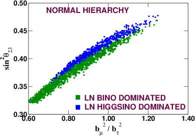
Refer to caption
Figure 2: Scatter plot of the neutrino mixing angle sin2θ23superscript2subscript𝜃23\sin^{2}\theta_{23} as a function of the ratio bμ2bτ2subscriptsuperscript𝑏2𝜇subscriptsuperscript𝑏2𝜏\frac{b^{2}_{\mu}}{b^{2}_{\tau}}. Values of other parameters are described in the text. The lightest neutralino (LN) is either bino or higgsino dominated.

5.2.2 Numerical Results

Let us first calculate the neutrino mixing angles for the parameter point discussed in Table 1. As we have discussed earlier, this parameter point generates the normal hierarchical pattern of neutrino masses. In Table 2, the three mixing angles are shown and they have been evaluated using the direct numerical calculation in eq.(26) as well as using the approximate analytical expressions in eq.(107). We want to emphasize once again that the approximate formulae have been used just to get some idea about the behaviours of the neutrino masses and mixing angles with various model parameters. This way we can identify the relevant parameters which crucially control the neutrino masses and mixing angles in different regions of the parameter space. However, these formulae are not valid everywhere in the allowed parameter space and in all the plots shown in this paper we have used full numerical calculation using eq.(26).

mixing angles in degree Using (26) Using (107)
θ12subscript𝜃12\theta_{12} 36.438 37.287
θ13subscript𝜃13\theta_{13} 9.424 6.428
θ23subscript𝜃23\theta_{23} 38.217 42.675
Table 2: Neutrino mixing angles for a sample parameter point discussed in Table 1. Results are shown using eq.(26) and eq.(107).

We have taken suitable values for λ𝜆\lambda and κ𝜅\kappa in such a way that they fall in the region allowed by the constraints in the scalar sector (similar to the region shown in fig. 1). We can see that for this choice of the parameter space, numerical and approximate analytical results give quite good agreement. Naturally, one would be interested to check the predictions made in eqs. (108), (109), and (110) over a wide region in the parameter space and see the deviations from the full numerical calculations. This has been shown in fig. 2, where we have plotted the value of sin2θ23superscript2subscript𝜃23\sin^{2}\theta_{23} as a function of the ratio bμ2/bτ2subscriptsuperscript𝑏2𝜇subscriptsuperscript𝑏2𝜏{b^{2}_{\mu}}/{b^{2}_{\tau}}.

We can see from this figure that for bμ2=bτ2subscriptsuperscript𝑏2𝜇subscriptsuperscript𝑏2𝜏b^{2}_{\mu}=b^{2}_{\tau}, the value of sin2θ23superscript2subscript𝜃23\sin^{2}\theta_{23} varies in the range 0.41 – 0.44, which corresponds to θ23subscript𝜃23\theta_{23} between 40 and 42. On the other hand, eq.(109) tells that for bμ2=bτ2subscriptsuperscript𝑏2𝜇subscriptsuperscript𝑏2𝜏b^{2}_{\mu}=b^{2}_{\tau}, sin2θ23=0.5.superscript2subscript𝜃230.5\sin^{2}\theta_{23}=0.5. So we see that in this case the result from the numerical calculation is reasonably close to the prediction from the approximate analytical formula. The choices for various parameters are given below. For the gaugino mass parameters M1subscript𝑀1M_{1} and M2subscript𝑀2M_{2}, we take two different sets of values which give us either a bino dominated lightest neutralino or a higgsino dominated lightest neutralino. In order to have a bino dominated lightest neutralino, our choices are M1=110GeV,M2=220GeVformulae-sequencesubscript𝑀1110GeVsubscript𝑀2220GeVM_{1}=110~{}{\rm GeV},M_{2}=220~{}{\rm GeV}, and for a higgsino dominated lightest neutralino we take M1=325GeV,M2=650GeVformulae-sequencesubscript𝑀1325GeVsubscript𝑀2650GeVM_{1}=325~{}{\rm GeV},M_{2}=650~{}{\rm GeV}. The same choices will be made for the gaugino mass parameters when we discuss the decays of the lightest neutralino in Sec. VI. Our choice of the ratio of the gaugino mass parameters at the electroweak scale is motivated by the assumption of universal gaugino mass at the grand unified theory scale. The value of κ𝜅\kappa is taken as 0.65 which satisfies the constraints from the scalar sector. We have taken two different values of λ𝜆\lambda corresponding to a bino or a higgsino dominated lightest neutralino. For the bino dominated case λ𝜆\lambda = 0.13, and for the higgsino dominated case λ𝜆\lambda = 0.06. The corresponding values for Aλλ=λ×1TeVsubscript𝐴𝜆𝜆𝜆1TeVA_{\lambda}\lambda=-\lambda\times 1{\rm TeV} and Aκκ=κ×1TeVsubscript𝐴𝜅𝜅𝜅1TeVA_{\kappa}\kappa=\kappa\times 1{\rm TeV}. The three diagonal neutrino Yukawa couplings (Yνiisuperscriptsubscript𝑌𝜈𝑖𝑖Y_{\nu}^{ii}) vary randomly in different ranges

3.55×1073.55superscript107\displaystyle 3.55\times 10^{-7} \displaystyle\leq Yν115.45×10⁷superscriptsubscript𝑌𝜈115.45superscript107\displaystyle Y_{\nu}^{11}\leq 5.45\times 10^{-7}
5.55×1075.55superscript107\displaystyle 5.55\times 10^{-7} \displaystyle\leq Yν226.65×10⁷superscriptsubscript𝑌𝜈226.65superscript107\displaystyle Y_{\nu}^{22}\leq 6.65\times 10^{-7}
1.45×1071.45superscript107\displaystyle 1.45\times 10^{-7} \displaystyle\leq Yν333.35×10⁷.superscriptsubscript𝑌𝜈333.35superscript107\displaystyle Y_{\nu}^{33}\leq 3.35\times 10^{-7}. (111)

The corresponding soft parameters (Aνiisuperscriptsubscript𝐴𝜈𝑖𝑖A_{\nu}^{ii}) also vary randomly in different ranges such that the parameters (AνYν)iisuperscriptsubscript𝐴𝜈subscript𝑌𝜈𝑖𝑖(A_{\nu}Y_{\nu})^{ii} effectively vary as follows

1.25×1041.25superscript104\displaystyle 1.25\times 10^{-4} \displaystyle\leq (AνYν)111.95×10⁴superscriptsubscript𝐴𝜈subscript𝑌𝜈111.95superscript104\displaystyle(A_{\nu}Y_{\nu})^{11}\leq 1.95\times 10^{-4}
3.45×1043.45superscript104\displaystyle 3.45\times 10^{-4} \displaystyle\leq (AνYν)224.95×10⁴superscriptsubscript𝐴𝜈subscript𝑌𝜈224.95superscript104\displaystyle(A_{\nu}Y_{\nu})^{22}\leq 4.95\times 10^{-4}
2.35×1042.35superscript104\displaystyle 2.35\times 10^{-4} \displaystyle\leq (AνYν)334.20×10⁴.superscriptsubscript𝐴𝜈subscript𝑌𝜈334.20superscript104\displaystyle(A_{\nu}Y_{\nu})^{33}\leq 4.20\times 10^{-4}. (112)

The allowed regions in the λκ𝜆𝜅\lambda-~{}\kappa plane are not very sensitive to the values of Yνsubscript𝑌𝜈Y_{\nu} and AνYνsubscript𝐴𝜈subscript𝑌𝜈A_{\nu}Y_{\nu} due to their smallness. Hence we choose them different for different cases, in order to accommodate the three flavour global neutrino data.
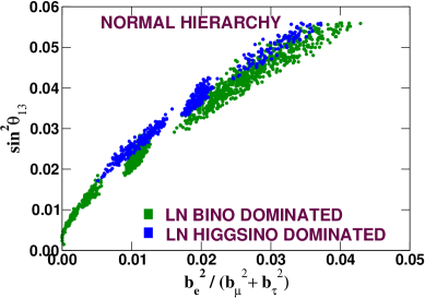
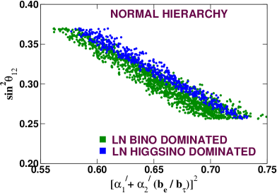
Refer to caption
Figure 3: sin2θ13superscript2subscript𝜃13\sin^{2}\theta_{13} as a function of the ratio be2bμ2+bτ2subscriptsuperscript𝑏2𝑒subscriptsuperscript𝑏2𝜇subscriptsuperscript𝑏2𝜏\frac{b^{2}_{e}}{b^{2}_{\mu}+b^{2}_{\tau}}. Values of other parameters are the same as in fig.2.
Refer to caption
Figure 4: sin2θ12superscript2subscript𝜃12\sin^{2}\theta_{12} as a function of (α1+α2bebτ)2superscriptsuperscriptsubscript𝛼1superscriptsubscript𝛼2subscript𝑏𝑒subscript𝑏𝜏2(\alpha_{1}^{\prime}+\alpha_{2}^{\prime}\frac{b_{e}}{b_{\tau}})^{2}. One can see that as (α1+α2bebτ)20.50superscriptsuperscriptsubscript𝛼1superscriptsubscript𝛼2subscript𝑏𝑒subscript𝑏𝜏20.50(\alpha_{1}^{\prime}+\alpha_{2}^{\prime}\frac{b_{e}}{b_{\tau}})^{2}\rightarrow 0.50, sin2θ12superscript2subscript𝜃12\sin^{2}\theta_{12} tends to 0.500.500.50, as predicted by the analytical formula. Values of other parameters are the same as in fig.2.

Note that in some parts of these ranges we have considered a bino dominated lightest neutralino and in some parts we have taken a higgsino dominated lightest neutralino with some overlapping regions. The values of other parameters are chosen to be mL~=400GeVsubscript𝑚~𝐿400GeVm_{\tilde{L}}=400~{}{\text{GeV}}, mν~c=300GeVsubscript𝑚superscript~𝜈𝑐300GeVm_{\tilde{\nu}^{c}}=300~{}{\text{GeV}} and tanβ=10.𝛽10\tan\beta=10. We have assumed that the phase δ𝛿\delta appearing in the mixing matrix (82) is zero. One important thing to notice is that even with a flavour diagonal structure of the neutrino Yukawa couplings Yνsubscript𝑌𝜈Y_{\nu}, one can obtain the required two large mixing angles for the neutrinos. The variations of other two mixing angles with the relevant parameters are shown in Figs. 4 and 4.

In fig.5, we have shown the regions in the various Yνsubscript𝑌𝜈Y_{\nu} planes satisfying the three flavour global neutrino data. The values of other parameters are as in fig.2 for the case where the lightest neutralino is bino dominated. We can see from these figures that the allowed values of Yνsubscript𝑌𝜈Y_{\nu}s show a mild hierarchy such that Yν22>Yν11>Yν33superscriptsubscript𝑌𝜈22superscriptsubscript𝑌𝜈11superscriptsubscript𝑌𝜈33Y_{\nu}^{22}>Y_{\nu}^{11}>Y_{\nu}^{33}.

Similar studies have been performed for the inverted hierarchical case and the allowed region shows that the magnitudes of the neutrino Yukawa couplings are larger compared to the case of normal hierarchical scheme of the neutrino masses with a different hierarchy among the Yνsubscript𝑌𝜈Y_{\nu}s themselves (Yν11>Yν22>Yν33superscriptsubscript𝑌𝜈11superscriptsubscript𝑌𝜈22superscriptsubscript𝑌𝜈33Y_{\nu}^{11}>Y_{\nu}^{22}>Y_{\nu}^{33}). In this case sin2θ12superscript2subscript𝜃12\sin^{2}\theta_{12} shows an increasing behaviour with the ratio be2/bμ2subscriptsuperscript𝑏2𝑒subscriptsuperscript𝑏2𝜇b^{2}_{e}/b^{2}_{\mu}, similar to the one shown by sin2θ23superscript2subscript𝜃23\sin^{2}\theta_{23} with bμ2/bτ2subscriptsuperscript𝑏2𝜇subscriptsuperscript𝑏2𝜏b^{2}_{\mu}/b^{2}_{\tau} in the normal hierarchical scenario. On the other hand, sin2θ23superscript2subscript𝜃23\sin^{2}\theta_{23} shows a decreasing behaviour with bμ2/bτ2subscriptsuperscript𝑏2𝜇subscriptsuperscript𝑏2𝜏b^{2}_{\mu}/b^{2}_{\tau}. In all these cases, the solar and atmospheric mass-squared differences are within the 3σ𝜎\sigma limits.

Refer to caption
Refer to caption
Refer to caption
Figure 5: Plots for normal hierarchical scheme of neutrino mass in Yν11Yν22subscriptsuperscript𝑌11𝜈subscriptsuperscript𝑌22𝜈Y^{11}_{\nu}~{}-~{}Y^{22}_{\nu}Yν11Yν33subscriptsuperscript𝑌11𝜈subscriptsuperscript𝑌33𝜈Y^{11}_{\nu}~{}-~{}Y^{33}_{\nu} and Yν22Yν33subscriptsuperscript𝑌22𝜈subscriptsuperscript𝑌33𝜈Y^{22}_{\nu}~{}-~{}Y^{33}_{\nu} plane when the lightest neutralino (LN) is bino dominated.

The case of νcsuperscript𝜈𝑐\nu^{c} dominated lightest neutralino has also been studied and it shows a very interesting and different behaviour compared to the bino and higgsino dominated cases. In this case, the dominant contribution in the neutrino mass matrix (eq.(47)) comes from the term proportional to aiajsubscript𝑎𝑖subscript𝑎𝑗a_{i}a_{j}. The terms proportional to bibjsubscript𝑏𝑖subscript𝑏𝑗b_{i}b_{j} should be considered as a perturbation. Hence, in the normal hierarchical scenario of neutrino masses, one would expect that sin2θ23superscript2subscript𝜃23\sin^{2}\theta_{23} is proportional to aμ2/aτ2subscriptsuperscript𝑎2𝜇subscriptsuperscript𝑎2𝜏a^{2}_{\mu}/a^{2}_{\tau}. This is exactly what we see in fig.6.

Note that for aμ2=aτ2subscriptsuperscript𝑎2𝜇subscriptsuperscript𝑎2𝜏a^{2}_{\mu}=a^{2}_{\tau}, the mixing becomes maximal. On the other hand, the solar mixing angle is controlled mostly by the quantity be2/bμ2subscriptsuperscript𝑏2𝑒subscriptsuperscript𝑏2𝜇b^{2}_{e}/b^{2}_{\mu} and shows an increasing behaviour with this ratio. In the case of inverted hierarchical scenario of neutrino masses, sin2θ23superscript2subscript𝜃23\sin^{2}\theta_{23} shows a decreasing behaviour with the ratio bμ2/bτ2subscriptsuperscript𝑏2𝜇subscriptsuperscript𝑏2𝜏b^{2}_{\mu}/b^{2}_{\tau} whereas sin2θ12superscript2subscript𝜃12\sin^{2}\theta_{12} shows an increasing pattern with be2/bμ2subscriptsuperscript𝑏2𝑒subscriptsuperscript𝑏2𝜇b^{2}_{e}/b^{2}_{\mu}. However, we do not show these plots here.

6 Decays of the lightest neutralino

Let us now look at some decay processes which can be considered as the typical consequence of this model. It is obvious that because of the R-parity violation there will be no stable lightest supersymmetric particle (LSP) present in this model. Here we consider the case where the lightest neutralino (χ~70subscriptsuperscript~𝜒07{\tilde{\chi}}^{0}_{7} in our notation to be described below) is the LSP (or NLSP in some cases) and study its decay pattern in the R-parity violating channels. In particular, we will consider the case where mχ~70>mW±subscript𝑚subscriptsuperscript~𝜒07subscript𝑚superscript𝑊plus-or-minusm_{{\tilde{\chi}}^{0}_{7}}>m_{W^{\pm}}, so that the three-body decays are less important compared to the two-body decays χ~70Z+νe,μ,τsubscriptsuperscript~𝜒07𝑍subscript𝜈𝑒𝜇𝜏{\tilde{\chi}}^{0}_{7}\rightarrow Z+\nu_{e,\mu,\tau}, χ~70W±+esubscriptsuperscript~𝜒07superscript𝑊plus-or-minussuperscript𝑒minus-or-plus{\tilde{\chi}}^{0}_{7}\rightarrow W^{\pm}+e^{\mp}, χ~70W±+μsubscriptsuperscript~𝜒07superscript𝑊plus-or-minussuperscript𝜇minus-or-plus{\tilde{\chi}}^{0}_{7}\rightarrow W^{\pm}+\mu^{\mp}, and χ~70W±+τsubscriptsuperscript~𝜒07superscript𝑊plus-or-minussuperscript𝜏minus-or-plus{\tilde{\chi}}^{0}_{7}\rightarrow W^{\pm}+\tau^{\mp}. The required Feynman rules for the computation of the decay of the lightest neutralino are given in the Appendix B. Let us also remark that the lightest neutralino LSP can also decay to h+ν𝜈h+\nu, if it is kinematically allowed, where hh is the MSSM-like lightest Higgs boson. However, for our illustration purposes we have considered the mass of the lightest neutralino in such a way that this decay is either kinematically forbidden or very much suppressed (assuming a lower bound on the mass of hh to be 114 GeV). Even if this decay branching ratio is slightly larger, it is usually smaller than the branching ratios in the (i+Wsubscript𝑖𝑊\ell_{i}+W) channel. Hence, this will not affect our conclusions regarding the ratios of branching ratios in the charged lepton channel (i+Wsubscript𝑖𝑊\ell_{i}+W), to be discussed later. The lightest neutralino decay χ~70ν+ν~csubscriptsuperscript~𝜒07𝜈superscript~𝜈𝑐{\tilde{\chi}}^{0}_{7}\rightarrow\nu+{\tilde{\nu}}^{c}, where ν~csuperscript~𝜈𝑐{\tilde{\nu}}^{c} is the scalar partner of the gauge singlet neutrino νcsuperscript𝜈𝑐\nu^{c}, is always very suppressed. We will discuss more on this when we consider a νcsuperscript𝜈𝑐\nu^{c} dominated lightest neutralino.

Consider the following decay process

χ~iχ~j+V,subscript~𝜒𝑖subscript~𝜒𝑗𝑉\tilde{\chi}_{i}\longrightarrow\tilde{\chi}_{j}+V, (113)

where χ~i(j)subscript~𝜒𝑖𝑗\tilde{\chi}_{i(j)} is either a neutralino or chargino, with mass mi(j)subscript𝑚𝑖𝑗m_{i(j)} and V𝑉V is the gauge boson which is either W±superscript𝑊plus-or-minusW^{\pm} or Z𝑍Z, with mass mvsubscript𝑚𝑣m_{v}. The masses misubscript𝑚𝑖m_{i} and mjsubscript𝑚𝑗m_{j} are positive.

The decay width for this process in eq.(113) is given by [23, 24]

Γ(χ~iχ~j+V)=g2𝒦1/232πmi3mW2×{(GL2+GR2)GLGR𝒢},Γsubscript~𝜒𝑖subscript~𝜒𝑗𝑉superscript𝑔2superscript𝒦1232𝜋subscriptsuperscript𝑚3𝑖subscriptsuperscript𝑚2𝑊subscriptsuperscript𝐺2𝐿subscriptsuperscript𝐺2𝑅subscriptsuperscript𝐺𝐿subscript𝐺𝑅𝒢\Gamma\left(\tilde{\chi}_{i}\longrightarrow\tilde{\chi}_{j}+V\right)=\frac{g^{2}\mathcal{K}^{1/2}}{32~{}\pi m^{3}_{i}m^{2}_{W}}\times\left\{\left(G^{2}_{L}+G^{2}_{R}\right)\mathcal{F}-G^{*}_{L}G_{R}~{}\mathcal{G}\right\},\\

where \mathcal{F}, 𝒢𝒢\mathcal{G} are functions of mi,mj,mvsubscript𝑚𝑖subscript𝑚𝑗subscript𝑚𝑣m_{i},m_{j},m_{v} and given by

(mi,mj,mv)=𝒦+3mv2(mi2+mj2mv2),subscript𝑚𝑖subscript𝑚𝑗subscript𝑚𝑣𝒦3subscriptsuperscript𝑚2𝑣subscriptsuperscript𝑚2𝑖subscriptsuperscript𝑚2𝑗subscriptsuperscript𝑚2𝑣\displaystyle\mathcal{F}(m_{i},m_{j},m_{v})=\mathcal{K}+3~{}m^{2}_{v}\left(m^{2}_{i}+m^{2}_{j}-m^{2}_{v}\right),
𝒢(mi,mj,mv)=12ϵiϵjmimjmv2,𝒢subscript𝑚𝑖subscript𝑚𝑗subscript𝑚𝑣12subscriptitalic-ϵ𝑖subscriptitalic-ϵ𝑗subscript𝑚𝑖subscript𝑚𝑗subscriptsuperscript𝑚2𝑣\displaystyle\mathcal{G}(m_{i},m_{j},m_{v})=12~{}\epsilon_{i}\epsilon_{j}m_{i}m_{j}m^{2}_{v},

with ϵi(j)subscriptitalic-ϵ𝑖𝑗\epsilon_{i}(j) carrying the actual signs (±1)plus-or-minus1(\pm 1) of the neutralino masses. The chargino masses must be positive. The kinematical factor 𝒦𝒦\mathcal{K} is given by

𝒦(mi2,mj2,mv2)=(mi2+mj2mv2)24mi2mj2.𝒦subscriptsuperscript𝑚2𝑖subscriptsuperscript𝑚2𝑗subscriptsuperscript𝑚2𝑣superscriptsubscriptsuperscript𝑚2𝑖subscriptsuperscript𝑚2𝑗subscriptsuperscript𝑚2𝑣24subscriptsuperscript𝑚2𝑖subscriptsuperscript𝑚2𝑗\mathcal{K}(m^{2}_{i},m^{2}_{j},m^{2}_{v})=\left(m^{2}_{i}+m^{2}_{j}-m^{2}_{v}\right)^{2}-4~{}m^{2}_{i}m^{2}_{j}. (115)
Refer to caption
Figure 6: Scatter plot of the neutrino mixing angle sin2θ23superscript2subscript𝜃23\sin^{2}\theta_{23} as a function of the ratio aμ2aτ2subscriptsuperscript𝑎2𝜇subscriptsuperscript𝑎2𝜏\frac{a^{2}_{\mu}}{a^{2}_{\tau}}. Values of other parameters are described in the text. The lightest neutralino (LN) is νcsuperscript𝜈𝑐\nu^{c} dominated.

In order to derive eq.(6), we have used the relation mW2=mZ2cos2θWsubscriptsuperscript𝑚2𝑊subscriptsuperscript𝑚2𝑍superscript2subscript𝜃𝑊m^{2}_{W}=m^{2}_{Z}\cos^{2}\theta_{W} and since ν~i<<v1,v2much-less-thandelimited-⟨⟩subscript~𝜈𝑖subscript𝑣1subscript𝑣2\langle\tilde{\nu}_{i}\rangle<<v_{1},v_{2}, some of the MSSM relations still hold good. The factors GLsubscript𝐺𝐿G_{L}, GRsubscript𝐺𝑅G_{R} are given here for some possible decay modes

Forχ~i0χ~j0ZForsubscriptsuperscript~𝜒0𝑖subscriptsuperscript~𝜒0𝑗𝑍\displaystyle\text{For}\quad\tilde{\chi}^{0}_{i}\longrightarrow\tilde{\chi}^{0}_{j}Z
GL=Oji′′L,GR=Oji′′R,formulae-sequencesubscript𝐺𝐿subscriptsuperscript𝑂′′𝐿𝑗𝑖subscript𝐺𝑅subscriptsuperscript𝑂′′𝑅𝑗𝑖\displaystyle G_{L}=O^{\prime\prime L}_{ji},\quad G_{R}=O^{\prime\prime R}_{ji},
Forχ~i0χ~j+WForsubscriptsuperscript~𝜒0𝑖subscriptsuperscript~𝜒𝑗superscript𝑊\displaystyle\text{For}\quad\tilde{\chi}^{0}_{i}\longrightarrow\tilde{\chi}^{+}_{j}{W^{-}}
GL=OijL,GR=OijR,formulae-sequencesubscript𝐺𝐿subscriptsuperscript𝑂𝐿𝑖𝑗subscript𝐺𝑅subscriptsuperscript𝑂𝑅𝑖𝑗\displaystyle G_{L}=O^{L}_{ij},\quad G_{R}=O^{R}_{ij},

where OijL(R)subscriptsuperscript𝑂𝐿𝑅𝑖𝑗O^{L(R)}_{ij} and Oji′′L(R)subscriptsuperscript𝑂′′𝐿𝑅𝑗𝑖O^{\prime\prime L(R)}_{ji} are given by eq.(B.1) and eq.(B.2).

Now consider the following decays

χ~LN0Z+ν,subscriptsuperscript~𝜒0𝐿𝑁𝑍𝜈\displaystyle\tilde{\chi}^{0}_{LN}\longrightarrow Z+\nu,
χ~LN0W±+,subscriptsuperscript~𝜒0𝐿𝑁superscript𝑊plus-or-minussuperscriptminus-or-plus\displaystyle\tilde{\chi}^{0}_{LN}\longrightarrow W^{\pm}+\ell^{\mp},

where χ~LN0subscriptsuperscript~𝜒0𝐿𝑁\tilde{\chi}^{0}_{LN} stands for lightest neutralino and =e,μ,τ𝑒𝜇𝜏\ell=e,\mu,\tau. At this stage let us discuss our notation and convention for these decays. The neutralino mass matrix is a 10×\times10 mass matrix which includes the left handed as well as the gauge-singlet neutrinos. If the mass eigenvalues of this matrix are arranged in the descending order then the three lightest eigenvalues of this 10×\times10 neutralino mass matrix would correspond to the three light neutrinos. Out of the remaining seven heavy eigenvalues, the lightest one is denoted as the lightest neutralino. Thus, in our notation χ~70subscriptsuperscript~𝜒07\tilde{\chi}^{0}_{7} is the lightest neutralino and χ~j+70,wheresubscriptsuperscript~𝜒0𝑗7where\tilde{\chi}^{0}_{j+7},\text{where} j=1,2,3𝑗123j=1,2,3 correspond to the three light neutrinos. Similarly, for the chargino masses, χ~l+2±subscriptsuperscript~𝜒plus-or-minus𝑙2\tilde{\chi}^{\pm}_{l+2} (l=1,2,3𝑙123l=1,2,3) corresponds to the charged leptons e,μ,τ𝑒𝜇𝜏e,\mu,\tau.

So for χ~LN0Z+νsubscriptsuperscript~𝜒0𝐿𝑁𝑍𝜈\tilde{\chi}^{0}_{LN}\rightarrow Z+\nu, which is also χ~70Z+χ~j+70subscriptsuperscript~𝜒07𝑍subscriptsuperscript~𝜒0𝑗7\tilde{\chi}^{0}_{7}\rightarrow Z+\tilde{\chi}^{0}_{j+7} (j=1,2,3𝑗123j=1,~{}2,~{}3), one gets from eq.(6) and eq.(B.1)

GL=12Nj+7,3N73+12Nj+7,4N7412Nj+7,k+7N7,k+7,subscript𝐺𝐿12subscript𝑁𝑗73subscriptsuperscript𝑁7312subscript𝑁𝑗74subscriptsuperscript𝑁7412subscript𝑁𝑗7𝑘7subscriptsuperscript𝑁7𝑘7\displaystyle G_{L}=-\frac{1}{2}N_{j+7,3}N^{*}_{73}+\frac{1}{2}N_{j+7,4}N^{*}_{74}-\frac{1}{2}N_{j+7,k+7}N^{*}_{7,k+7},
GR=GL,subscript𝐺𝑅subscriptsuperscript𝐺𝐿\displaystyle G_{R}=-G^{*}_{L},

where j,k=1,2,3formulae-sequence𝑗𝑘123~{}j,k=1,~{}2,~{}3 and this in turn modifies eq.(6) as

Γ(χ~70Z+χ~j+70)=g2𝒦1/232πmχ~703mW2×{2GL2+GL2𝒢},Γsubscriptsuperscript~𝜒07𝑍subscriptsuperscript~𝜒0𝑗7superscript𝑔2superscript𝒦1232𝜋subscriptsuperscript𝑚3subscriptsuperscript~𝜒07subscriptsuperscript𝑚2𝑊2subscriptsuperscript𝐺2𝐿subscriptsuperscript𝐺superscript2𝐿𝒢\Gamma\left(\tilde{\chi}^{0}_{7}\rightarrow Z+~{}\tilde{\chi}^{0}_{j+7}\right)=\frac{g^{2}\mathcal{K}^{1/2}}{32~{}\pi m^{3}_{{\tilde{\chi}}^{0}_{7}}m^{2}_{W}}\times\left\{2~{}G^{2}_{L}\mathcal{F}+G^{*^{2}}_{L}~{}\mathcal{G}\right\}, (119)

with mi=mχ~70subscript𝑚𝑖subscript𝑚subscriptsuperscript~𝜒07m_{i}=m_{{\tilde{\chi}}^{0}_{7}}, mj=mν0subscript𝑚𝑗subscript𝑚𝜈0m_{j}=m_{\nu}\approx 0 and mv=mZsubscript𝑚𝑣subscript𝑚𝑍m_{v}=m_{Z}.

Let us now consider the other decay which is χ~LN0W±+subscriptsuperscript~𝜒0𝐿𝑁superscript𝑊plus-or-minussuperscriptminus-or-plus\tilde{\chi}^{0}_{LN}\rightarrow W^{\pm}+\ell^{\mp} or equivalently χ~70W±+χ~j(j=3,4,5)subscriptsuperscript~𝜒07superscript𝑊plus-or-minussubscriptsuperscript~𝜒minus-or-plus𝑗𝑗345\tilde{\chi}^{0}_{7}\rightarrow W^{\pm}+\tilde{\chi}^{\mp}_{j}(j=3,4,5).

For the process χ~70W+χ~j+subscriptsuperscript~𝜒07superscript𝑊subscriptsuperscript~𝜒𝑗\tilde{\chi}^{0}_{7}\rightarrow W^{-}+\tilde{\chi}^{+}_{j}

Γ(χ~70W+χ~j+)=g2𝒦1/232πmχ~703mW2×{(GL2+GR2)GLGR𝒢},Γsubscriptsuperscript~𝜒07superscript𝑊subscriptsuperscript~𝜒𝑗superscript𝑔2superscript𝒦1232𝜋subscriptsuperscript𝑚3subscriptsuperscript~𝜒07subscriptsuperscript𝑚2𝑊subscriptsuperscript𝐺2𝐿subscriptsuperscript𝐺2𝑅subscriptsuperscript𝐺𝐿subscript𝐺𝑅𝒢\displaystyle\Gamma\left(\tilde{\chi}^{0}_{7}\rightarrow W^{-}+~{}\tilde{\chi}^{+}_{j}\right)=\frac{g^{2}\mathcal{K}^{1/2}}{32~{}\pi m^{3}_{{\tilde{\chi}}^{0}_{7}}m^{2}_{W}}\times\left\{\left(G^{2}_{L}+G^{2}_{R}\right)\mathcal{F}-G^{*}_{L}G_{R}~{}\mathcal{G}\right\},
GL=N72Vj112N74Vj2,subscript𝐺𝐿subscript𝑁72subscriptsuperscript𝑉𝑗112subscript𝑁74subscriptsuperscript𝑉𝑗2\displaystyle G_{L}=N_{72}V^{*}_{j1}-\frac{1}{\sqrt{2}}N_{74}V^{*}_{j2},
GR=N72Uj1+12N73Uj2+12N7,k+7Uj,k+2,subscript𝐺𝑅subscriptsuperscript𝑁72subscript𝑈𝑗112subscriptsuperscript𝑁73subscript𝑈𝑗212subscriptsuperscript𝑁7𝑘7subscript𝑈𝑗𝑘2\displaystyle G_{R}=N^{*}_{72}U_{j1}+\frac{1}{\sqrt{2}}N^{*}_{73}U_{j2}+\frac{1}{\sqrt{2}}N^{*}_{7,k+7}U_{j,k+2},
(k=1,2,3),𝑘123\displaystyle(k=1,~{}2,~{}3), (120)

where eq.(6) and eq.(B.2) has been used. The process χ~70W++χ~jsubscriptsuperscript~𝜒07superscript𝑊subscriptsuperscript~𝜒𝑗\tilde{\chi}^{0}_{7}\longrightarrow W^{+}+\tilde{\chi}^{-}_{j} is obtained by charge conjugation of the process in eq.(6).

6.1 Correlation between the lightest neutralino decays and neutrino mixing angles

Correlations between the lightest neutralino decays and neutrino mixing angles will depend on the nature of the lightest neutralino as well as on the mass hierarchies of the neutrinos, i.e. whether we have a normal hierarchical pattern of neutrino masses or an inverted one. In this section we look into these possibilities in details and consider three different cases for the dominant component of the lightest neutralino. We consider that the lightest neutralino is (1) bino dominated, (2) higgsino dominated, and (3) νcsuperscript𝜈𝑐\nu^{c} dominated. For each of these cases we consider both the normal and the inverted hierarchical pattern of neutrino masses. We show that in these different cases, the ratio of branching ratios of certain decays of the lightest neutralino correlates with the neutrino mixing angles. In some cases the correlation is with the atmospheric and the reactor angle and in other cases the ratio of the branching ratios correlates with the solar mixing angle and in some cases there is no correlations at all. Let us now study these possibilities case by case. The interesting difference between this study and similar studies with bilinear R-parity violating scenario [25] in the MSSM is the presence of a gauge singlet neutrino dominated lightest neutralino. We will see later that in this case the results can be very different from the bino or higgsino dominated lightest neutralino. The lightest neutralino decays in neutrino mass models with spontaneous R-parity violation have been studied in ref.[26].

6.1.1 Bino dominated lightest neutralino

We will assume that the gaugino masses are unified at the grand unified theory (GUT) scale. At the EW scale the ratio of the U(1)𝑈1U(1) and SU(2)𝑆𝑈2SU(2) gaugino masses are M1/M2=1:2:subscript𝑀1subscript𝑀212M_{1}/M_{2}=1:2. If in addition, M1<μsubscript𝑀1𝜇M_{1}<\mu and the value of κ𝜅\kappa is large (so that the effective gauge singlet neutrino mass 2κνc2𝜅superscript𝜈𝑐2\kappa\nu^{c} is large), the lightest neutralino is essentially bino dominated and it is the LSP. First we consider the case when the composition of the lightest neutralino is such that, the bino-component |N71|2>superscriptsubscript𝑁712absent|N_{71}|^{2}> 0.92 and neutrino masses follow the normal hierarchical pattern. We have observed that for the bino dominated case, the lightest neutralino (χ~70subscriptsuperscript~𝜒07{\tilde{\chi}}^{0}_{7}) couplings to ±superscriptplus-or-minus\ell^{\pm}Wsuperscript𝑊minus-or-plusW^{\mp} pair (where =e,μ𝑒𝜇\ell=e,\mu or τ𝜏\tau) depend on the quantities bisubscript𝑏𝑖b_{i} along with a factor which is independent of various lepton generations. Naturally, we would expect that the ratios of various decay branching ratios such as BR(χ~70e+Wsubscriptsuperscript~𝜒07𝑒𝑊{\tilde{\chi}}^{0}_{7}\rightarrow e+W), BR(χ~70μ+Wsubscriptsuperscript~𝜒07𝜇𝑊{\tilde{\chi}}^{0}_{7}\rightarrow\mu+W), and BR(χ~70τ+Wsubscriptsuperscript~𝜒07𝜏𝑊{\tilde{\chi}}^{0}_{7}\rightarrow\tau+W) show nice correlations with the quantities bi2/bj2subscriptsuperscript𝑏2𝑖subscriptsuperscript𝑏2𝑗b^{2}_{i}/b^{2}_{j} with i,j being e,μ𝑒𝜇e,\mu or τ𝜏\tau. This feature is evident from fig.7. Here we have scanned the parameter space of the three neutrino Yukawa couplings with random values for a particular choice of the couplings λ𝜆\lambda, κ𝜅\kappa and the associated soft SUSY breaking trilinear parameters, as well as other MSSM parameters. The trilinear soft parameters Aνsubscript𝐴𝜈A_{\nu} corresponding to Yνsubscript𝑌𝜈Y_{\nu}s also vary randomly in a certain range. In addition we have imposed the condition that the lightest neutralino (which is the LSP) is bino dominated and neutrino mass pattern is normal hierarchical.
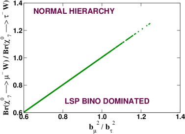
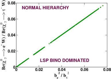
Refer to caption
Refer to caption
Refer to caption
Figure 7: Ratio Br(χ70iW)Br(χ70jW)𝐵𝑟subscriptsuperscript𝜒07subscript𝑖𝑊𝐵𝑟subscriptsuperscript𝜒07subscript𝑗𝑊\frac{Br(\chi^{0}_{7}\longrightarrow\ell_{i}~{}W)}{Br(\chi^{0}_{7}\longrightarrow\ell_{j}~{}W)} versus bi2bj2subscriptsuperscript𝑏2𝑖subscriptsuperscript𝑏2𝑗\frac{b^{2}_{i}}{b^{2}_{j}} plot for a bino like lightest neutralino (the LSP) with bino component, |N71|2>superscriptsubscript𝑁712absent|N_{71}|^{2}> 0.92, where i,j,k=e,μ,τformulae-sequence𝑖𝑗𝑘𝑒𝜇𝜏i,j,k~{}=~{}e,\mu,\tau. Neutrino mass pattern is taken to be normal hierarchical. Choice of parameters are M1=110subscript𝑀1110M_{1}=110 GeV, λ=0.13,κ=0.65,mν~c=300GeVandmL~=400GeVformulae-sequence𝜆0.13formulae-sequence𝜅0.65subscript𝑚superscript~𝜈𝑐300GeVandsubscript𝑚~𝐿400GeV\lambda=0.13,\kappa=0.65,m_{\tilde{\nu}^{c}}=300~{}{\rm GeV}~{}{\rm and}~{}m_{\tilde{L}}=400~{}{\rm GeV}. Mass of the LSP is 106.9 GeV. The value of the μ𝜇\mu parameter comes out to be -228.9 GeV.
Refer to caption
Refer to caption
Figure 8: Ratio Br(χ70μW)Br(χ70τW)𝐵𝑟subscriptsuperscript𝜒07𝜇𝑊𝐵𝑟subscriptsuperscript𝜒07𝜏𝑊\frac{Br(\chi^{0}_{7}\longrightarrow\mu~{}W)}{Br(\chi^{0}_{7}\longrightarrow\tau~{}W)} versus tan2θ23superscript2subscript𝜃23\tan^{2}\theta_{23} (left), Br(χ70eW)Br(χ70μW)2+Br(χ70τW)2𝐵𝑟subscriptsuperscript𝜒07𝑒𝑊𝐵𝑟superscriptsubscriptsuperscript𝜒07𝜇𝑊2𝐵𝑟superscriptsubscriptsuperscript𝜒07𝜏𝑊2\frac{Br(\chi^{0}_{7}\longrightarrow e~{}W)}{\sqrt{Br(\chi^{0}_{7}\longrightarrow\mu~{}W)^{2}+Br(\chi^{0}_{7}\longrightarrow\tau~{}W)^{2}}} with tan2θ13superscript2subscript𝜃13\tan^{2}\theta_{13} (right) plot for a bino dominated lightest neutralino (the LSP) with bino component, |N71|2>superscriptsubscript𝑁712absent|N_{71}|^{2}> 0.92. Neutrino mass pattern is normal hierarchical. Choice of parameters are same as that of fig.7.
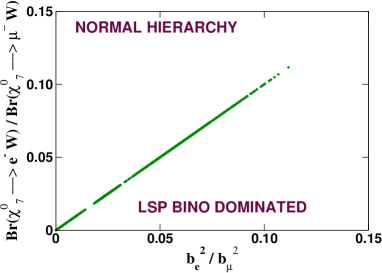
We have checked that the correlations between the ratios of the lightest neutralino decay branching ratios and bi2/bj2subscriptsuperscript𝑏2𝑖subscriptsuperscript𝑏2𝑗b^{2}_{i}/b^{2}_{j} is more prominent with increasing bino component of the lightest neutralino. Note that when (bi/bj)21superscriptsubscript𝑏𝑖subscript𝑏𝑗21(b_{i}/b_{j})^{2}\rightarrow 1 the ratios of branching ratios shown in fig.7 also tend to 111. We have seen earlier that the neutrino mixing angles θ23subscript𝜃23\theta_{23} and θ13subscript𝜃13\theta_{13} also show nice correlation with the ratios bμ2/bτ2subscriptsuperscript𝑏2𝜇subscriptsuperscript𝑏2𝜏b^{2}_{\mu}/b^{2}_{\tau} and be2/bτ2subscriptsuperscript𝑏2𝑒subscriptsuperscript𝑏2𝜏b^{2}_{e}/b^{2}_{\tau}, respectively (see Figs.2 and 4). Hence we would expect that the ratios of the branching ratios BR(χ~70μW)BR(χ~70τW)BRsubscriptsuperscript~𝜒07𝜇𝑊BRsubscriptsuperscript~𝜒07𝜏𝑊\frac{{\rm BR}({\tilde{\chi}}^{0}_{7}\rightarrow\mu W)}{{\rm BR}({\tilde{\chi}}^{0}_{7}\rightarrow\tau W)} and BR(χ~70eW)BR(χ~70μW)2+BR(χ~70τW)2𝐵𝑅subscriptsuperscript~𝜒07𝑒𝑊𝐵𝑅superscriptsubscriptsuperscript~𝜒07𝜇𝑊2𝐵𝑅superscriptsubscriptsuperscript~𝜒07𝜏𝑊2\frac{BR({\tilde{\chi}}^{0}_{7}\longrightarrow e~{}W)}{\sqrt{BR({\tilde{\chi}}^{0}_{7}\longrightarrow\mu~{}W)^{2}+BR({\tilde{\chi}}^{0}_{7}\longrightarrow\tau~{}W)^{2}}} show correlations with tan2θ23superscript2subscript𝜃23\tan^{2}\theta_{23} and tan2θ13superscript2subscript𝜃13\tan^{2}\theta_{13}. These correlations are shown in fig.8. We have seen earlier (see eq.(75)) that with the normal hierarchical pattern of the neutrino masses, the atmospheric mass scale is determined by the quantity Ωb=be2+bμ2+bτ2subscriptΩ𝑏subscriptsuperscript𝑏2𝑒subscriptsuperscript𝑏2𝜇subscriptsuperscript𝑏2𝜏\Omega_{b}=\sqrt{b^{2}_{e}+b^{2}_{\mu}+b^{2}_{\tau}}. Naturally one would expect that the atmospheric and the reactor angles are correlated with the +W𝑊\ell+W final states of the lightest neutralino decays and no correlation is expected for the solar angle. This is what we have observed numerically. Here we have considered the regions of the parameter space where the neutrino mass-squared differences and mixing angles are within the 3σ𝜎\sigma allowed range shown in eqs.(1)–(3). fig.8 also shows the model prediction for the ratios of branching ratios where the neutrino experimental data are satisfied. For our sample choice of parameters in fig.8, one would expect that the ratio BR(χ~70μW)BR(χ~70τW)𝐵𝑅subscriptsuperscript~𝜒07𝜇𝑊𝐵𝑅subscriptsuperscript~𝜒07𝜏𝑊\frac{BR({\tilde{\chi}}^{0}_{7}\longrightarrow\mu~{}W)}{BR({\tilde{\chi}}^{0}_{7}\longrightarrow\tau~{}W)} should be in the range 0.45 to 1.25. Similarly, the other ratio BR(χ~70eW)BR(χ~70μW)2+BR(χ~70τW)2𝐵𝑅subscriptsuperscript~𝜒07𝑒𝑊𝐵𝑅superscriptsubscriptsuperscript~𝜒07𝜇𝑊2𝐵𝑅superscriptsubscriptsuperscript~𝜒07𝜏𝑊2\frac{BR({\tilde{\chi}}^{0}_{7}\longrightarrow e~{}W)}{\sqrt{BR({\tilde{\chi}}^{0}_{7}\longrightarrow\mu~{}W)^{2}+BR({\tilde{\chi}}^{0}_{7}\longrightarrow\tau~{}W)^{2}}} is expected in this case to be less than 0.07. We can also see from fig.8 that the ratio of branching ratios in the (μ+W𝜇𝑊\mu+W) and (τ+W𝜏𝑊\tau+W) channels becomes almost equal for the maximal value of the atmospheric mixing angle (θ23=45subscript𝜃23superscript45\theta_{23}~{}=~{}45^{\circ}). On the other hand, we do not observe any correlation with the solar mixing angle θ12subscript𝜃12\theta_{12} since it is a complicated function of ai2subscriptsuperscript𝑎2𝑖a^{2}_{i} and bi2subscriptsuperscript𝑏2𝑖b^{2}_{i} (see eq. (110)).

Refer to caption
Refer to caption
Refer to caption
Figure 9: Ratio BR(χ~70iW)BR(χ~70jW)𝐵𝑅subscriptsuperscript~𝜒07subscriptsuperscript𝑖𝑊𝐵𝑅subscriptsuperscript~𝜒07subscriptsuperscript𝑗𝑊\frac{BR({\tilde{\chi}}^{0}_{7}\longrightarrow\ell^{-}_{i}~{}W)}{BR({\tilde{\chi}}^{0}_{7}\longrightarrow\ell^{-}_{j}~{}W)} versus bi2bj2subscriptsuperscript𝑏2𝑖subscriptsuperscript𝑏2𝑗\frac{b^{2}_{i}}{b^{2}_{j}} plot for a bino like lightest neutralino (the LSP) with bino component |N71|2>superscriptsubscript𝑁712absent|N_{71}|^{2}> 0.95, where i,j,k=e,μ,τformulae-sequence𝑖𝑗𝑘𝑒𝜇𝜏i,j,k~{}=~{}e,\mu,\tau. Neutrino mass pattern is inverted hierarchical. Choice of parameters are M1=105subscript𝑀1105M_{1}=105 GeV, λ=0.15,κ=0.65,mν~c=300GeVandmL~=445GeVformulae-sequence𝜆0.15formulae-sequence𝜅0.65subscript𝑚superscript~𝜈𝑐300GeVandsubscript𝑚~𝐿445GeV\lambda=0.15,\kappa=0.65,m_{\tilde{\nu}^{c}}=300~{}{\rm GeV}~{}{\rm and}~{}m_{\tilde{L}}=445~{}{\rm GeV}. Mass of the LSP is 103.3 GeV. The value of the μ𝜇\mu parameter comes out to be -263.7 GeV.

In the case of inverted hierarchical mass pattern of the light neutrinos, the χ~70subscriptsuperscript~𝜒07{\tilde{\chi}}^{0}_{7}isubscript𝑖\ell_{i}W𝑊W coupling is still controlled by the quantities bi2subscriptsuperscript𝑏2𝑖b^{2}_{i}. Hence the ratios of the branching ratios discussed earlier, show nice correlations with bi2/bj2subscriptsuperscript𝑏2𝑖subscriptsuperscript𝑏2𝑗b^{2}_{i}/b^{2}_{j} (see fig.9). However, in this case the solar mixing angle shows some correlation with the ratio BR(χ~70eW)BR(χ~70μW)2+BR(χ~70τW)2𝐵𝑅subscriptsuperscript~𝜒07𝑒𝑊𝐵𝑅superscriptsubscriptsuperscript~𝜒07𝜇𝑊2𝐵𝑅superscriptsubscriptsuperscript~𝜒07𝜏𝑊2\frac{BR({\tilde{\chi}}^{0}_{7}\longrightarrow e~{}W)}{\sqrt{BR({\tilde{\chi}}^{0}_{7}\longrightarrow\mu~{}W)^{2}+BR({\tilde{\chi}}^{0}_{7}\longrightarrow\tau~{}W)^{2}}}. This is shown in fig.10. The correlation is not very sharp and some dispersion occurs due to the fact that the two heavier neutrino masses controlling the atmospheric mass scale and solar mass-squared difference are not completely determined by the quantities bi2subscriptsuperscript𝑏2𝑖b^{2}_{i} and there is some contribution of the quantities ai2subscriptsuperscript𝑎2𝑖a^{2}_{i}, particularly for the second heavy neutrino mass eigenstate.

Refer to caption
Refer to caption
Figure 10: Ratio BR(χ~70eW)BR(χ~70μW)2+BR(χ~70τW)2𝐵𝑅subscriptsuperscript~𝜒07𝑒𝑊𝐵𝑅superscriptsubscriptsuperscript~𝜒07𝜇𝑊2𝐵𝑅superscriptsubscriptsuperscript~𝜒07𝜏𝑊2\frac{BR({\tilde{\chi}}^{0}_{7}\longrightarrow e~{}W)}{\sqrt{BR({\tilde{\chi}}^{0}_{7}\longrightarrow\mu~{}W)^{2}+BR({\tilde{\chi}}^{0}_{7}\longrightarrow\tau~{}W)^{2}}} with tan2θ12superscript2subscript𝜃12\tan^{2}\theta_{12} (left) plot for a bino dominated lightest neutralino (LSP) with bino component |N71|2>superscriptsubscript𝑁712absent|N_{71}|^{2}> 0.95. In the right figure the ratio BR(χ~70μW)BR(χ~70τW)𝐵𝑅subscriptsuperscript~𝜒07𝜇𝑊𝐵𝑅subscriptsuperscript~𝜒07𝜏𝑊\frac{BR({\tilde{\chi}}^{0}_{7}\longrightarrow\mu~{}W)}{BR({\tilde{\chi}}^{0}_{7}\longrightarrow\tau~{}W)} versus tan2θ23superscript2subscript𝜃23\tan^{2}\theta_{23} is plotted. Neutrino mass pattern is assumed to be inverted hierarchical. Choice of parameters are same as that of fig.9.

The correlation of the ratio BR(χ~70μW)BR(χ~70τW)𝐵𝑅subscriptsuperscript~𝜒07𝜇𝑊𝐵𝑅subscriptsuperscript~𝜒07𝜏𝑊\frac{BR({\tilde{\chi}}^{0}_{7}\longrightarrow\mu~{}W)}{BR({\tilde{\chi}}^{0}_{7}\longrightarrow\tau~{}W)} with tan2θ23superscript2subscript𝜃23\tan^{2}\theta_{23} shows a different behaviour compared to what we have seen in the case of normal hierarchical scenario. This is because in the case of inverted hierarchical mass pattern of the neutrinos, tan2θ23superscript2subscript𝜃23\tan^{2}\theta_{23} decreases with increasing bμ2/bτ2subscriptsuperscript𝑏2𝜇subscriptsuperscript𝑏2𝜏b^{2}_{\mu}/b^{2}_{\tau}. One can observe from Figs.8 and 10 that if the experimental value of the ratio BR(χ~70eW)BR(χ~70μW)2+BR(χ~70τW)2𝐵𝑅subscriptsuperscript~𝜒07𝑒𝑊𝐵𝑅superscriptsubscriptsuperscript~𝜒07𝜇𝑊2𝐵𝑅superscriptsubscriptsuperscript~𝜒07𝜏𝑊2\frac{BR({\tilde{\chi}}^{0}_{7}\longrightarrow e~{}W)}{\sqrt{BR({\tilde{\chi}}^{0}_{7}\longrightarrow\mu~{}W)^{2}+BR({\tilde{\chi}}^{0}_{7}\longrightarrow\tau~{}W)^{2}}} is much-less-than\ll 1 then that indicates a normal hierarchical neutrino mass pattern for a bino-dominated lightest neutralino LSP whereas a higher value (similar-to\sim 1) of this ratio measured in experiments might indicate that the neutrino mass pattern is inverted hierarchical. Similarly a measurement of the ratio BR(χ~70μW)BR(χ~70τW)𝐵𝑅subscriptsuperscript~𝜒07𝜇𝑊𝐵𝑅subscriptsuperscript~𝜒07𝜏𝑊\frac{BR({\tilde{\chi}}^{0}_{7}\longrightarrow\mu~{}W)}{BR({\tilde{\chi}}^{0}_{7}\longrightarrow\tau~{}W)} can also give an indication regarding the particular hierarchy of the neutrino mass pattern in the case of a bino dominated LSP.

6.1.2 Higgsino dominated lightest neutralino

When one considers higher values of the U(1)𝑈1U(1) gaugino mass M1subscript𝑀1M_{1}, i.e. M1>μsubscript𝑀1𝜇M_{1}>\mu and large value of κ𝜅\kappa (so that the effective gauge singlet neutrino mass 2κνc2𝜅superscript𝜈𝑐2\kappa\nu^{c} is large), the lightest neutralino is essentially higgsino dominated and it is the LSP. Naturally one needs to consider a small value of the coupling λ𝜆\lambda so that the effective μ𝜇\mu parameter (μ=3λνc𝜇3𝜆superscript𝜈𝑐\mu=3\lambda\nu^{c}) is smaller. In order to look at the lightest neutralino decay branching ratios in this case, we consider a situation where the higgsino component in χ~70subscriptsuperscript~𝜒07{\tilde{\chi}}^{0}_{7} is |N73|2+|N74|2>superscriptsubscript𝑁732superscriptsubscript𝑁742absent|N_{73}|^{2}+|N_{74}|^{2}> 0.90. As in the case of a bino dominated LSP, the generation dependence of the χ~70subscriptsuperscript~𝜒07{\tilde{\chi}}^{0}_{7}isubscript𝑖\ell_{i}W𝑊W couplings comes through the quantities bi2subscriptsuperscript𝑏2𝑖b^{2}_{i}. However, because of the large value of the τ𝜏\tau Yukawa coupling, the higgsino–τ𝜏\tau mixing is larger and as a result the partial decay width of χ~70subscriptsuperscript~𝜒07{\tilde{\chi}}^{0}_{7} into (W+τ𝑊𝜏W+\tau) is larger than into (W+μ𝑊𝜇W+\mu) and (W+e𝑊𝑒W+e). This feature is shown in fig.11, where the ratios of branching ratios are plotted against the quantities bi2/bj2subscriptsuperscript𝑏2𝑖subscriptsuperscript𝑏2𝑗b^{2}_{i}/b^{2}_{j}. The domination of BR(χ~70τ+Wsubscriptsuperscript~𝜒07𝜏𝑊{\tilde{\chi}}^{0}_{7}\rightarrow\tau+W) over the other two is clearly evident. Nevertheless, all the three ratios of branching ratios show sharp correlations with the corresponding bi2/bj2subscriptsuperscript𝑏2𝑖subscriptsuperscript𝑏2𝑗b^{2}_{i}/b^{2}_{j}. In this figure the normal hierarchical pattern of the neutrino masses has been considered. As in the case of a bino LSP, here also the ratios BR(χ~70μW)BR(χ~70τW)𝐵𝑅subscriptsuperscript~𝜒07𝜇𝑊𝐵𝑅subscriptsuperscript~𝜒07𝜏𝑊\frac{BR({\tilde{\chi}}^{0}_{7}\longrightarrow\mu~{}W)}{BR({\tilde{\chi}}^{0}_{7}\longrightarrow\tau~{}W)} and BR(χ~70eW)BR(χ~70μW)2+BR(χ~70τW)2𝐵𝑅subscriptsuperscript~𝜒07𝑒𝑊𝐵𝑅superscriptsubscriptsuperscript~𝜒07𝜇𝑊2𝐵𝑅superscriptsubscriptsuperscript~𝜒07𝜏𝑊2\frac{BR({\tilde{\chi}}^{0}_{7}\longrightarrow e~{}W)}{\sqrt{BR({\tilde{\chi}}^{0}_{7}\longrightarrow\mu~{}W)^{2}+BR({\tilde{\chi}}^{0}_{7}\longrightarrow\tau~{}W)^{2}}} show nice correlations with neutrino mixing angles θ23subscript𝜃23\theta_{23} and θ13subscript𝜃13\theta_{13}, respectively. This is shown in fig.12. However, in this case the predictions for these two ratios are very different from the bino LSP case. The expected value of the ratio BR(χ~70μW)BR(χ~70τW)𝐵𝑅subscriptsuperscript~𝜒07𝜇𝑊𝐵𝑅subscriptsuperscript~𝜒07𝜏𝑊\frac{BR({\tilde{\chi}}^{0}_{7}\longrightarrow\mu~{}W)}{BR({\tilde{\chi}}^{0}_{7}\longrightarrow\tau~{}W)} is approximately between 0.05 and 0.10 in a region where one can accommodate the experimental neutrino data. Similarly, the predicted value of the ratio BR(χ~70eW)BR(χ~70μW)2+BR(χ~70τW)2𝐵𝑅subscriptsuperscript~𝜒07𝑒𝑊𝐵𝑅superscriptsubscriptsuperscript~𝜒07𝜇𝑊2𝐵𝑅superscriptsubscriptsuperscript~𝜒07𝜏𝑊2\frac{BR({\tilde{\chi}}^{0}_{7}\longrightarrow e~{}W)}{\sqrt{BR({\tilde{\chi}}^{0}_{7}\longrightarrow\mu~{}W)^{2}+BR({\tilde{\chi}}^{0}_{7}\longrightarrow\tau~{}W)^{2}}} is \leq 0.006. On the other hand, there is no such correlations with the solar mixing angle θ12subscript𝜃12\theta_{12}.

Refer to caption
Refer to caption
Refer to caption
Figure 11: Ratio BR(χ~70liW)BR(χ~70ljW)𝐵𝑅subscriptsuperscript~𝜒07subscript𝑙𝑖𝑊𝐵𝑅subscriptsuperscript~𝜒07subscript𝑙𝑗𝑊\frac{BR({\tilde{\chi}}^{0}_{7}\longrightarrow l_{i}~{}W)}{BR({\tilde{\chi}}^{0}_{7}\longrightarrow l_{j}~{}W)} versus bi2bj2subscriptsuperscript𝑏2𝑖subscriptsuperscript𝑏2𝑗\frac{b^{2}_{i}}{b^{2}_{j}} plot for a higgsino like LSP with higgsino component (|N73|2+|N74|2)>superscriptsubscript𝑁732superscriptsubscript𝑁742absent(|N_{73}|^{2}+|N_{74}|^{2})> 0.95, where i,j,k=e,μ,τformulae-sequence𝑖𝑗𝑘𝑒𝜇𝜏i,j,k~{}=~{}e,\mu,\tau. Neutrino mass pattern is normal hierarchical. Choice of parameters are M1=325subscript𝑀1325M_{1}=325 GeV, λ=0.06,κ=0.65,mν~c=300GeVandmL~=400GeVformulae-sequence𝜆0.06formulae-sequence𝜅0.65subscript𝑚superscript~𝜈𝑐300GeVandsubscriptm~L400GeV\lambda=0.06,\kappa=0.65,m_{\tilde{\nu}^{c}}=300~{}{\rm GeV}~{}\rm{and}~{}m_{\tilde{L}}=400~{}{\rm GeV}. Mass of the LSP is 98.6 GeV. The value of the μ𝜇\mu parameter comes out to be -105.9 GeV.
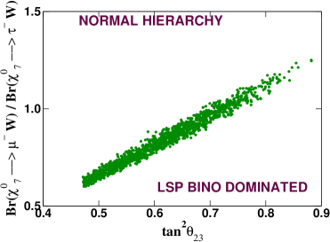
Refer to caption
Refer to caption
Figure 12: Ratio BR(χ~70μW)BR(χ~70τW)𝐵𝑅subscriptsuperscript~𝜒07𝜇𝑊𝐵𝑅subscriptsuperscript~𝜒07𝜏𝑊\frac{BR({\tilde{\chi}}^{0}_{7}\longrightarrow\mu~{}W)}{BR({\tilde{\chi}}^{0}_{7}\longrightarrow\tau~{}W)} versus tan2θ23superscript2subscript𝜃23\tan^{2}\theta_{23}  (left), BR(χ~70eW)BR(χ~70μW)2+BR(χ~70τW)2𝐵𝑅subscriptsuperscript~𝜒07𝑒𝑊𝐵𝑅superscriptsubscriptsuperscript~𝜒07𝜇𝑊2𝐵𝑅superscriptsubscriptsuperscript~𝜒07𝜏𝑊2\frac{BR({\tilde{\chi}}^{0}_{7}\longrightarrow e~{}W)}{\sqrt{BR({\tilde{\chi}}^{0}_{7}\longrightarrow\mu~{}W)^{2}+BR({\tilde{\chi}}^{0}_{7}\longrightarrow\tau~{}W)^{2}}} with tan2θ13superscript2subscript𝜃13\tan^{2}\theta_{13}  (right) plot for a higgsino LSP with higgsino component (|N73|2+|N74|2)>superscriptsubscript𝑁732superscriptsubscript𝑁742absent(|N_{73}|^{2}+|N_{74}|^{2})> 0.95. Neutrino mass pattern is normal hierarchical. Choice of parameters are same as that of fig.11.
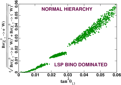
Similar correlations of the ratios of branching ratios with bi2/bj2subscriptsuperscript𝑏2𝑖subscriptsuperscript𝑏2𝑗b^{2}_{i}/b^{2}_{j} are also obtained for a higgsino dominated LSP in the case where the neutrino mass pattern is inverted hierarchical. Once again it shows that the χ~70subscriptsuperscript~𝜒07{\tilde{\chi}}^{0}_{7} decays to (τ+W𝜏𝑊\tau+W) channel is dominant over the channels (e+W𝑒𝑊e+W) and (μ+W𝜇𝑊\mu+W) for any values of bi2/bj2subscriptsuperscript𝑏2𝑖subscriptsuperscript𝑏2𝑗b^{2}_{i}/b^{2}_{j} because of the larger τ𝜏\tau Yukawa coupling. On the other hand, the correlations with the neutrino mixing angles show a behaviour similar to that of a bino LSP with inverted neutrino mass hierarchy though with much smaller values for the ratios BR(χ~70μW)BR(χ~70τW)𝐵𝑅subscriptsuperscript~𝜒07𝜇𝑊𝐵𝑅subscriptsuperscript~𝜒07𝜏𝑊\frac{BR({\tilde{\chi}}^{0}_{7}\rightarrow\mu~{}W)}{BR({\tilde{\chi}}^{0}_{7}\rightarrow\tau~{}W)} and BR(χ~70eW)BR(χ~70μW)2+Br(χ~70τW)2𝐵𝑅subscriptsuperscript~𝜒07𝑒𝑊𝐵𝑅superscriptsubscriptsuperscript~𝜒07𝜇𝑊2𝐵𝑟superscriptsubscriptsuperscript~𝜒07𝜏𝑊2\frac{BR({\tilde{\chi}}^{0}_{7}\rightarrow e~{}W)}{\sqrt{BR({\tilde{\chi}}^{0}_{7}\rightarrow\mu~{}W)^{2}+Br({\tilde{\chi}}^{0}_{7}\rightarrow\tau~{}W)^{2}}}. These are shown in fig.13. Note that the correlations in this case are not very sharp, especially with tan2θ12superscript2subscript𝜃12\tan^{2}\theta_{12}. Thus we see that small values of these ratios (for both normal and inverted hierarchy) are characteristic features of a higgsino dominated LSP in this model.

6.1.3 νcsuperscript𝜈𝑐\nu^{c} dominated lightest neutralino

Because of our choice of parameters i.e., a generation independent coupling κ𝜅\kappa of the gauge singlet neutrinos and a common VEV νcsuperscript𝜈𝑐\nu^{c}, the three neutralino mass eigenstates which are predominantly gauge singlet neutrinos are essentially mass degenerate. There is a very small mass splitting due to mixing. However, unlike the case of a bino or higgsino dominated lightest neutralino, these νcsuperscript𝜈𝑐\nu^{c} dominated lightest neutralino states cannot be considered as the LSP. This is because in this case the lightest scalar (which is predominantly a gauge singlet sneutrino ν~csuperscript~𝜈𝑐{\tilde{\nu}}^{c}) is the lightest supersymmetric particle. This is very interesting since usually one does not get a ν~csuperscript~𝜈𝑐{\tilde{\nu}}^{c} as an LSP in a model where the gauge singlet neutrino superfield has a large Majorana mass term in the superpotential. However, in this case the effective Majorana mass term is at the EW scale and there is also a contribution from the trilinear scalar coupling Aκκsubscript𝐴𝜅𝜅A_{\kappa}\kappa which keeps the mass of the singlet scalar sneutrino smaller. It is also very interesting to study the decay patterns of the lightest neutralino in this case since here one can probe the gauge singlet neutrino mass scales at the colliders.
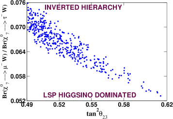
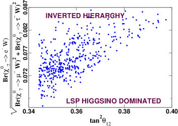
Refer to caption
Refer to caption
Figure 13: Ratio BR(χ~70μW)BR(χ~70τW)𝐵𝑅subscriptsuperscript~𝜒07𝜇𝑊𝐵𝑅subscriptsuperscript~𝜒07𝜏𝑊\frac{BR({\tilde{\chi}}^{0}_{7}\longrightarrow\mu~{}W)}{BR({\tilde{\chi}}^{0}_{7}\longrightarrow\tau~{}W)} versus tan2θ23superscript2subscript𝜃23\tan^{2}\theta_{23}  (left), BR(χ~70eW)BR(χ~70μW)2+Br(χ~70τW)2𝐵𝑅subscriptsuperscript~𝜒07𝑒𝑊𝐵𝑅superscriptsubscriptsuperscript~𝜒07𝜇𝑊2𝐵𝑟superscriptsubscriptsuperscript~𝜒07𝜏𝑊2\frac{BR({\tilde{\chi}}^{0}_{7}\longrightarrow e~{}W)}{\sqrt{BR({\tilde{\chi}}^{0}_{7}\longrightarrow\mu~{}W)^{2}+Br({\tilde{\chi}}^{0}_{7}\longrightarrow\tau~{}W)^{2}}} with tan2θ12superscript2subscript𝜃12\tan^{2}\theta_{12} (right) plot for a higgsino LSP with higgsino component (|N73|2+|N74|2)>superscriptsubscript𝑁732superscriptsubscript𝑁742absent(|N_{73}|^{2}+|N_{74}|^{2})> 0.95. Neutrino mass pattern is inverted hierarchical. Choice of parameters are M1=490subscript𝑀1490M_{1}=490 GeV, λ=0.07,κ=0.65,mν~c=320GeVandmL~=430GeVformulae-sequence𝜆0.07formulae-sequence𝜅0.65subscript𝑚superscript~𝜈𝑐320GeVandsubscriptm~L430GeV\lambda=0.07,\kappa=0.65,m_{\tilde{\nu}^{c}}=320\rm{GeV}~{}\rm{and}~{}m_{\tilde{L}}=430\rm{GeV}. Mass of the LSP is 110.8 GeV. The value of the μ𝜇\mu parameter comes out to be -115.3 GeV.

Before discussing the decay patterns of the lightest neutralino which is νcsuperscript𝜈𝑐\nu^{c} dominated, let us say a few words regarding their production at the LHC. The direct production of νcsuperscript𝜈𝑐\nu^{c} (by νcsuperscript𝜈𝑐\nu^{c} we mean the νcsuperscript𝜈𝑐\nu^{c} dominated lightest neutralino in this section) is negligible because of the very small mixing with the MSSM neutralinos. Nevertheless, they can be produced at the end of the cascade decay chains of the squarks and gluinos at the LHC. For example, if the next-to-next-to-lightest SUSY particle (NNLSP) is higgsino dominated (this is the state above the three almost degenerate lightest neutralinos) and it has a non-negligible mixing with νcsuperscript𝜈𝑐\nu^{c} (remember that the higgsino–νcsuperscript𝜈𝑐\nu^{c} mixing occurs mainly because of the term λν^cH^1H^2𝜆superscript^𝜈𝑐subscript^𝐻1subscript^𝐻2\lambda{\hat{\nu}}^{c}{\hat{H}}_{1}{\hat{H}}_{2} in the superpotential), then the branching ratio of the decay H~Z+νc~𝐻𝑍superscript𝜈𝑐{\tilde{H}}\rightarrow Z+\nu^{c} can be larger than the branching ratios in the W𝑊\ell W and νZ𝜈𝑍\nu Z channels. This way one can produce νcsuperscript𝜈𝑐\nu^{c} dominated lightest neutralino. Similarly, a higgsino dominated lighter chargino can also produce gauge singlet neutrinos. Another way of producing νcsuperscript𝜈𝑐\nu^{c} is through the decay of an NNLSP τ~1subscript~𝜏1{\tilde{\tau}}_{1}, such as τ~1τ+νcsubscript~𝜏1𝜏superscript𝜈𝑐{\tilde{\tau}}_{1}\rightarrow\tau+\nu^{c}. A detailed discussion of these issues is beyond the scope of the present paper and we hope to come back to this in a future publication [27].
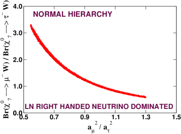
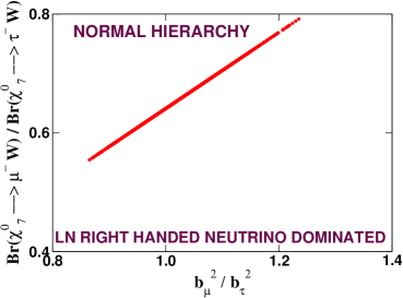
Refer to caption
Refer to caption
Figure 14: Ratio BR(χ~70μW)BR(χ~70τW)𝐵𝑅subscriptsuperscript~𝜒07𝜇𝑊𝐵𝑅subscriptsuperscript~𝜒07𝜏𝑊\frac{BR({\tilde{\chi}}^{0}_{7}\longrightarrow\mu~{}W)}{BR({\tilde{\chi}}^{0}_{7}\longrightarrow\tau~{}W)} versus aμ2aτ2subscriptsuperscript𝑎2𝜇subscriptsuperscript𝑎2𝜏\frac{a^{2}_{\mu}}{a^{2}_{\tau}} (left) and versus bμ2bτ2subscriptsuperscript𝑏2𝜇subscriptsuperscript𝑏2𝜏\frac{b^{2}_{\mu}}{b^{2}_{\tau}} (right) plot for a νcsuperscript𝜈𝑐\nu^{c} like lightest neutralino (χ~70subscriptsuperscript~𝜒07{\tilde{\chi}}^{0}_{7}) with νcsuperscript𝜈𝑐\nu^{c} component (|N75|2+|N76|2+|N77|2)>superscriptsubscript𝑁752superscriptsubscript𝑁762superscriptsubscript𝑁772absent(|N_{75}|^{2}+|N_{76}|^{2}+|N_{77}|^{2})> 0.99, (left) and >>0.97 (right). Neutrino mass pattern is normal hierarchical. Choice of parameters are for (left) M1=405subscript𝑀1405M_{1}=405 GeV, λ=0.29,κ=0.07,(Aλλ)=8.2TeV×λ,(Aκκ)=165GeV×κ,mν~c=50GeVandmL~=825GeVformulae-sequence𝜆0.29formulae-sequence𝜅0.07formulae-sequencesubscript𝐴𝜆𝜆8.2TeV𝜆formulae-sequencesubscript𝐴𝜅𝜅165GeV𝜅subscript𝑚superscript~𝜈𝑐50GeVandsubscriptm~L825GeV\lambda=0.29,\kappa=0.07,(A_{\lambda}\lambda)=-8.2~{}{\rm TeV}\times\lambda,(A_{\kappa}\kappa)=165~{}{\rm GeV}\times\kappa,~{}m_{\tilde{\nu}^{c}}=50~{}{\rm GeV}~{}\rm{and}~{}m_{\tilde{L}}=825~{}{\rm GeV} and for (right) M1=405subscript𝑀1405M_{1}=405 GeV, λ=0.10,κ=0.07,(Aλλ)=2TeV×λ,(Aκκ)=165GeV×κ,mν~c=50GeVandmL~=825GeVformulae-sequence𝜆0.10formulae-sequence𝜅0.07formulae-sequencesubscript𝐴𝜆𝜆2TeV𝜆formulae-sequencesubscript𝐴𝜅𝜅165GeV𝜅subscript𝑚superscript~𝜈𝑐50GeVandsubscript𝑚~𝐿825GeV\lambda=0.10,\kappa=0.07,(A_{\lambda}\lambda)=-2~{}{\rm TeV}\times\lambda,(A_{\kappa}\kappa)=165~{}{\rm GeV}\times\kappa,~{}m_{\tilde{\nu}^{c}}=50~{}{\rm GeV}~{}{\rm and}~{}m_{\tilde{L}}=825~{}{\rm GeV}. Mass of the lightest neutralino is 129.4 GeV (left) and 119.8 GeV (right) respectively. The values of the μ𝜇\mu parameter are -803.9 GeV and -258.8 GeV, respectively.

When one considers higher value of the gaugino mass, i.e. M1>μsubscript𝑀1𝜇M_{1}>\mu and a small value of the coupling κ𝜅\kappa (so that the effective Majorana mass of νcsuperscript𝜈𝑐\nu^{c} is small, i.e. 2κνc<μ2𝜅superscript𝜈𝑐𝜇2\kappa\nu^{c}<\mu), the lightest neutralino is essentially νcsuperscript𝜈𝑐\nu^{c} dominated. As we have mentioned earlier, in this case the LSP is the scalar partner of νcsuperscript𝜈𝑐\nu^{c}, i.e. ν~csuperscript~𝜈𝑐{\tilde{\nu}}^{c}. However, the decay of νcsuperscript𝜈𝑐\nu^{c} into ν+ν~c𝜈superscript~𝜈𝑐\nu+{\tilde{\nu}}^{c} is suppressed compared to the decays νci+Wsuperscript𝜈𝑐subscript𝑖𝑊\nu^{c}\rightarrow\ell_{i}+W and νcνi+Zsuperscript𝜈𝑐subscript𝜈𝑖𝑍\nu^{c}\rightarrow\nu_{i}+Z that we have considered so far. Because of this in this section we will neglect the decay νcν+ν~csuperscript𝜈𝑐𝜈superscript~𝜈𝑐\nu^{c}\rightarrow\nu+{\tilde{\nu}}^{c} while discussing the correlation of the lightest neutralino (χ~70subscriptsuperscript~𝜒07{\tilde{\chi}}^{0}_{7}) decays with the neutrino mixing angles.

In this case the coupling of the lightest neutralino (χ~70subscriptsuperscript~𝜒07{\tilde{\chi}}^{0}_{7}) with isubscript𝑖\ell_{i}W𝑊W pair depends on the νcsuperscript𝜈𝑐\nu^{c} content of χ~70subscriptsuperscript~𝜒07{\tilde{\chi}}^{0}_{7}. Note that the νcsuperscript𝜈𝑐\nu^{c} has a very small mixing with the MSSM neutralino states. However, in some cases the νcsuperscript𝜈𝑐\nu^{c} dominated lightest neutralino can have a non-negligible higgsino component. In such cases the coupling χ~70subscriptsuperscript~𝜒07{\tilde{\chi}}^{0}_{7}isubscript𝑖\ell_{i}W𝑊W depends mainly on the quantities bisubscript𝑏𝑖b_{i}. On the other hand, if χ~70subscriptsuperscript~𝜒07{\tilde{\chi}}^{0}_{7} is very highly dominated by νcsuperscript𝜈𝑐\nu^{c}, then the coupling χ~70subscriptsuperscript~𝜒07{\tilde{\chi}}^{0}_{7}isubscript𝑖\ell_{i}W𝑊W has a nice correlation with the quantities aisubscript𝑎𝑖a_{i}. So in order to study the decay correlations of the νcsuperscript𝜈𝑐\nu^{c} dominated lightest neutralino, we consider two cases (i) νcsuperscript𝜈𝑐\nu^{c} component is >> 0.99, and (ii) νcsuperscript𝜈𝑐\nu^{c} component is >0.97absent0.97>0.97 with some non-negligible higgsino admixture.

The correlations of the decay branching ratio BR(χ~70μW)BR(χ~70τW)𝐵𝑅subscriptsuperscript~𝜒07𝜇𝑊𝐵𝑅subscriptsuperscript~𝜒07𝜏𝑊\frac{BR({\tilde{\chi}}^{0}_{7}\longrightarrow\mu~{}W)}{BR({\tilde{\chi}}^{0}_{7}\longrightarrow\tau~{}W)} are shown in fig.14 for the cases (i) and (ii) mentioned above. As we have explained already, this figure demonstrates that in case (i) the ratio of the branching ratio is dependent on the quantity aμ2/aτ2subscriptsuperscript𝑎2𝜇subscriptsuperscript𝑎2𝜏a^{2}_{\mu}/a^{2}_{\tau} whereas in case (ii) this ratio is correlated with bμ2/bτ2subscriptsuperscript𝑏2𝜇subscriptsuperscript𝑏2𝜏b^{2}_{\mu}/b^{2}_{\tau} though there is some suppression due to large τ𝜏\tau Yukawa coupling.

Refer to caption
Refer to caption
Figure 15: Ratio BR(χ~70eW)BR(χ~70μW)𝐵𝑅subscriptsuperscript~𝜒07𝑒𝑊𝐵𝑅subscriptsuperscript~𝜒07𝜇𝑊\frac{BR({\tilde{\chi}}^{0}_{7}\longrightarrow e~{}W)}{BR({\tilde{\chi}}^{0}_{7}\longrightarrow\mu~{}W)} versus ae2aμ2subscriptsuperscript𝑎2𝑒subscriptsuperscript𝑎2𝜇\frac{a^{2}_{e}}{a^{2}_{\mu}} (left) and versus be2bμ2subscriptsuperscript𝑏2𝑒subscriptsuperscript𝑏2𝜇\frac{b^{2}_{e}}{b^{2}_{\mu}} (right) plot for a νcsuperscript𝜈𝑐\nu^{c} like lightest neutralino (χ~70subscriptsuperscript~𝜒07{\tilde{\chi}}^{0}_{7}) with νcsuperscript𝜈𝑐\nu^{c} component (|N75|2+|N76|2+|N77|2)>superscriptsubscript𝑁752superscriptsubscript𝑁762superscriptsubscript𝑁772absent(|N_{75}|^{2}+|N_{76}|^{2}+|N_{77}|^{2})> 0.99 (left), and >>0.97 (right). Neutrino mass pattern is normal hierarchical. Choice of parameters are same as that of fig.14.

Similar calculations were performed also for the other ratios discussed earlier. For example, in fig.15 we have shown the variations of the ratio BR(χ~70eW)BR(χ~70μW)𝐵𝑅subscriptsuperscript~𝜒07𝑒𝑊𝐵𝑅subscriptsuperscript~𝜒07𝜇𝑊\frac{BR({\tilde{\chi}}^{0}_{7}\longrightarrow e~{}W)}{BR({\tilde{\chi}}^{0}_{7}\longrightarrow\mu~{}W)} as functions of ae2aμ2subscriptsuperscript𝑎2𝑒subscriptsuperscript𝑎2𝜇\frac{a^{2}_{e}}{a^{2}_{\mu}} and be2bμ2subscriptsuperscript𝑏2𝑒subscriptsuperscript𝑏2𝜇\frac{b^{2}_{e}}{b^{2}_{\mu}} for the cases (i) and (ii), respectively. The variation with ae2aμ2subscriptsuperscript𝑎2𝑒subscriptsuperscript𝑎2𝜇\frac{a^{2}_{e}}{a^{2}_{\mu}} is not sharp and dispersive in nature whereas the variation with be2bμ2subscriptsuperscript𝑏2𝑒subscriptsuperscript𝑏2𝜇\frac{b^{2}_{e}}{b^{2}_{\mu}} is very sharp and shows that in this case the relevant couplings are proportional to besubscript𝑏𝑒b_{e} and bμsubscript𝑏𝜇b_{\mu}, respectively.

Refer to caption
Refer to caption
Figure 16: Ratio BR(χ~70μW)BR(χ~70τW)𝐵𝑅subscriptsuperscript~𝜒07𝜇𝑊𝐵𝑅subscriptsuperscript~𝜒07𝜏𝑊\frac{BR({\tilde{\chi}}^{0}_{7}\longrightarrow\mu~{}W)}{BR({\tilde{\chi}}^{0}_{7}\longrightarrow\tau~{}W)} versus tan2θ23superscript2subscript𝜃23\tan^{2}\theta_{23} (left), BR(χ~70eW)BR(χ~70μW)2+BR(χ~70τW)2𝐵𝑅subscriptsuperscript~𝜒07𝑒𝑊𝐵𝑅superscriptsubscriptsuperscript~𝜒07𝜇𝑊2𝐵𝑅superscriptsubscriptsuperscript~𝜒07𝜏𝑊2\frac{BR({\tilde{\chi}}^{0}_{7}\longrightarrow e~{}W)}{\sqrt{BR({\tilde{\chi}}^{0}_{7}\longrightarrow\mu~{}W)^{2}+BR({\tilde{\chi}}^{0}_{7}\longrightarrow\tau~{}W)^{2}}} with tan2θ12superscript2subscript𝜃12\tan^{2}\theta_{12}  (right) plot for a νcsuperscript𝜈𝑐\nu^{c} dominated lightest neutralino with νcsuperscript𝜈𝑐\nu^{c} component (|N75|2+|N76|2+|N77|2)>superscriptsubscript𝑁752superscriptsubscript𝑁762superscriptsubscript𝑁772absent(|N_{75}|^{2}+|N_{76}|^{2}+|N_{77}|^{2})> 0.99 (left) and >> 0.97 (right). Neutrino mass pattern is normal hierarchical. Choice of parameters are same as that of fig.14.

On the other hand, in case (i) only tan2θ23superscript2subscript𝜃23\tan^{2}\theta_{23} shows a nice correlation with the ratio BR(χ~70μW)BR(χ~70τW)𝐵𝑅subscriptsuperscript~𝜒07𝜇𝑊𝐵𝑅subscriptsuperscript~𝜒07𝜏𝑊\frac{BR({\tilde{\chi}}^{0}_{7}\longrightarrow\mu~{}W)}{BR({\tilde{\chi}}^{0}_{7}\longrightarrow\tau~{}W)} (see fig.16) and tan2θ12superscript2subscript𝜃12\tan^{2}\theta_{12} or tan2θ13superscript2subscript𝜃13\tan^{2}\theta_{13} does not show any correlation with the other ratio. The non-linear behaviour of the ratios of branching ratios in case(i) is due to the fact that the parameters Yνsubscript𝑌𝜈Y_{\nu}s (which control the aisubscript𝑎𝑖a_{i}) appear both in the neutralino and chargino mass matrices. The charged lepton Yukawa couplings also play a role in determining the ratios. One can also see that the prediction for this ratio of branching ratio for case (i), as shown in fig.16, is in the range 0.5–3.5, which is larger compared to the bino dominated or higgsino dominated cases for both normal and inverted hierarchical pattern of neutrino masses. Also, the nature of this variation is similar to what we see with the inverted hierarchical pattern of neutrino masses in the bino or higgsino dominated cases.

In case (ii) none of the neutrino mixing angles show very good correlations with the ratios of branching ratios that we have been discussing. However, one can still observe some kind of a correlation of the ratio BR(χ~70eW)BR(χ~70μW)2+BR(χ~70τW)2𝐵𝑅subscriptsuperscript~𝜒07𝑒𝑊𝐵𝑅superscriptsubscriptsuperscript~𝜒07𝜇𝑊2𝐵𝑅superscriptsubscriptsuperscript~𝜒07𝜏𝑊2\frac{BR({\tilde{\chi}}^{0}_{7}\longrightarrow e~{}W)}{\sqrt{BR({\tilde{\chi}}^{0}_{7}\longrightarrow\mu~{}W)^{2}+BR({\tilde{\chi}}^{0}_{7}\longrightarrow\tau~{}W)^{2}}} with tan2θ12superscript2subscript𝜃12\tan^{2}\theta_{12}. The prediction for this ratio from the neutrino data is on the smaller side (similar-to\sim 0.07).

Refer to caption
Refer to caption
Figure 17: Ratio BR(χ~70μW)BR(χ~70τW)𝐵𝑅subscriptsuperscript~𝜒07𝜇𝑊𝐵𝑅subscriptsuperscript~𝜒07𝜏𝑊\frac{BR({\tilde{\chi}}^{0}_{7}\longrightarrow\mu~{}W)}{BR({\tilde{\chi}}^{0}_{7}\longrightarrow\tau~{}W)} versus aμ2aτ2subscriptsuperscript𝑎2𝜇subscriptsuperscript𝑎2𝜏\frac{a^{2}_{\mu}}{a^{2}_{\tau}} (left) and versus bμ2bτ2subscriptsuperscript𝑏2𝜇subscriptsuperscript𝑏2𝜏\frac{b^{2}_{\mu}}{b^{2}_{\tau}} (right) plot for a νcsuperscript𝜈𝑐\nu^{c} like lightest neutralino (χ~70subscriptsuperscript~𝜒07{\tilde{\chi}}^{0}_{7}) with νcsuperscript𝜈𝑐\nu^{c} component (|N75|2+|N76|2+|N77|2)>superscriptsubscript𝑁752superscriptsubscript𝑁762superscriptsubscript𝑁772absent(|N_{75}|^{2}+|N_{76}|^{2}+|N_{77}|^{2})> 0.99 (left), and >>0.97 (right). Neutrino mass pattern is inverted hierarchical. Choice of parameters are for (left) M1=445subscript𝑀1445M_{1}=445 GeV, λ=0.29,κ=0.07,(Aλλ)=8.2TeV×λ,(Aκκ)=165GeV×κ,mν~c=50GeVandmL~=835GeVformulae-sequence𝜆0.29formulae-sequence𝜅0.07formulae-sequencesubscript𝐴𝜆𝜆8.2TeV𝜆formulae-sequencesubscript𝐴𝜅𝜅165GeV𝜅subscript𝑚superscript~𝜈𝑐50GeVandsubscript𝑚~𝐿835GeV\lambda=0.29,\kappa=0.07,(A_{\lambda}\lambda)=-8.2~{}{\rm TeV}\times\lambda,(A_{\kappa}\kappa)=165~{}{\rm GeV}\times\kappa,~{}m_{\tilde{\nu}^{c}}=50~{}{\rm GeV}~{}{\rm and}~{}m_{\tilde{L}}=835\rm{GeV} and for (right) M1=445subscript𝑀1445M_{1}=445 GeV, λ=0.10,κ=0.07,(Aλλ)=2TeV×λ,(Aκκ)=165GeV×κ,mν~c=50GeVandmL~=835GeVformulae-sequence𝜆0.10formulae-sequence𝜅0.07formulae-sequencesubscript𝐴𝜆𝜆2TeV𝜆formulae-sequencesubscript𝐴𝜅𝜅165GeV𝜅subscript𝑚superscript~𝜈𝑐50GeVandsubscript𝑚~𝐿835GeV\lambda=0.10,\kappa=0.07,(A_{\lambda}\lambda)=-2~{}{\rm TeV}\times\lambda,(A_{\kappa}\kappa)=165~{}{\rm GeV}\times\kappa,~{}m_{\tilde{\nu}^{c}}=50~{}{\rm GeV}~{}{\rm and}~{}m_{\tilde{L}}=835~{}{\rm GeV}. Mass of the lightest neutralino is 129.4 GeV (left) and 119.8 GeV (right) respectively.

With the inverted hierarchical neutrino mass pattern, in case (i) one observes a sharp correlation of the ratio BR(χ~70μW)BR(χ~70τW)𝐵𝑅subscriptsuperscript~𝜒07𝜇𝑊𝐵𝑅subscriptsuperscript~𝜒07𝜏𝑊\frac{BR({\tilde{\chi}}^{0}_{7}\longrightarrow\mu~{}W)}{BR({\tilde{\chi}}^{0}_{7}\longrightarrow\tau~{}W)} with aμ2aτ2subscriptsuperscript𝑎2𝜇subscriptsuperscript𝑎2𝜏\frac{a^{2}_{\mu}}{a^{2}_{\tau}} (see fig.17). The other two ratios BR(χ~70eW)BR(χ~70μW)𝐵𝑅subscriptsuperscript~𝜒07𝑒𝑊𝐵𝑅subscriptsuperscript~𝜒07𝜇𝑊\frac{BR({\tilde{\chi}}^{0}_{7}\longrightarrow e~{}W)}{BR({\tilde{\chi}}^{0}_{7}\longrightarrow\mu~{}W)} and BR(χ~70eW)BR(χ~70τW)𝐵𝑅subscriptsuperscript~𝜒07𝑒𝑊𝐵𝑅subscriptsuperscript~𝜒07𝜏𝑊\frac{BR({\tilde{\chi}}^{0}_{7}\longrightarrow e~{}W)}{BR({\tilde{\chi}}^{0}_{7}\longrightarrow\tau~{}W)} do not show very sharp correlations with ae2aμ2subscriptsuperscript𝑎2𝑒subscriptsuperscript𝑎2𝜇\frac{a^{2}_{e}}{a^{2}_{\mu}} and ae2aτ2subscriptsuperscript𝑎2𝑒subscriptsuperscript𝑎2𝜏\frac{a^{2}_{e}}{a^{2}_{\tau}}, respectively and we do not plot them here. However, in case (ii) all the three ratios show nice correlations with the corresponding bi2/bj2subscriptsuperscript𝑏2𝑖subscriptsuperscript𝑏2𝑗b^{2}_{i}/b^{2}_{j}. We have shown this in fig.17 only for bμ2/bτ2subscriptsuperscript𝑏2𝜇subscriptsuperscript𝑏2𝜏b^{2}_{\mu}/b^{2}_{\tau}. In this case the variations of the ratios of branching ratios with neutrino mixing angles are shown in fig.18.
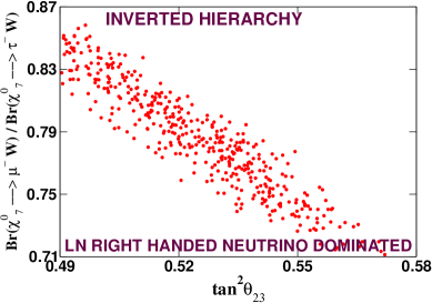
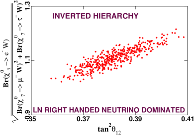
Refer to caption
Refer to caption
Figure 18: Ratio BR(χ~70μW)BR(χ~70τW)𝐵𝑅subscriptsuperscript~𝜒07𝜇𝑊𝐵𝑅subscriptsuperscript~𝜒07𝜏𝑊\frac{BR({\tilde{\chi}}^{0}_{7}\longrightarrow\mu~{}W)}{BR({\tilde{\chi}}^{0}_{7}\longrightarrow\tau~{}W)} versus tan2θ23superscript2subscript𝜃23\tan^{2}\theta_{23}  (left), BR(χ~70eW)BR(χ~70μW)2+BR(χ~70τW)2𝐵𝑅subscriptsuperscript~𝜒07𝑒𝑊𝐵𝑅superscriptsubscriptsuperscript~𝜒07𝜇𝑊2𝐵𝑅superscriptsubscriptsuperscript~𝜒07𝜏𝑊2\frac{BR({\tilde{\chi}}^{0}_{7}\longrightarrow e~{}W)}{\sqrt{BR({\tilde{\chi}}^{0}_{7}\longrightarrow\mu~{}W)^{2}+BR({\tilde{\chi}}^{0}_{7}\longrightarrow\tau~{}W)^{2}}} with tan2θ12superscript2subscript𝜃12\tan^{2}\theta_{12}  (right) plot for a νcsuperscript𝜈𝑐\nu^{c} dominated lightest neutralino with νcsuperscript𝜈𝑐\nu^{c} component (|N75|2+|N76|2+|N77|2)>superscriptsubscript𝑁752superscriptsubscript𝑁762superscriptsubscript𝑁772absent(|N_{75}|^{2}+|N_{76}|^{2}+|N_{77}|^{2})> 0.97. Neutrino mass pattern is inverted hierarchical. Choice of parameters are same as that of fig.17.

For the case (i), only tan2θ13superscript2subscript𝜃13\tan^{2}\theta_{13} shows certain correlation with the ratio of branching ratio shown in fig.18 (right), but we do not show it here.

Finally, we would like to mention that in all these different cases discussed above, the lightest neutralino can have a finite decay length which can produce displaced vertices in the vertex detectors. Depending on the composition of the lightest neutralino, one can have different decay lengths. For example, a bino-dominated lightest neutralino can produce a displaced vertex similar-to\sim a few mm. Similarly, for a higgsino dominated lightest neutralino, decay vertices of the order of a few cms can be observed. On the other hand, if the lightest neutralino is νcsuperscript𝜈𝑐\nu^{c} dominated, then the decay lengths can be of the order of a few meters. These are very unique predictions of this model which can, in principle, be tested at the LHC.

7 Summary and Conclusion

In this work we have studied a supersymmetric model in detail where the observed pattern of neutrino mass-squared differences and mixing angles are obtained with the help of three standard model gauge-singlet neutrino superfields, which simultaneously solve the μ𝜇\mu problem of MSSM. The additional terms in the superpotential and the scalar potential include R-parity violating interactions involving these gauge-singlet neutrino superfields. The vacuum expectation values of the singlet sneutrinos give rise to effective Majorana mass terms for the singlet neutrinos, as well as a μ𝜇\mu-term, both at the electroweak scale. This model was introduced in ref.[8] and some phenomenology was discussed for a single gauge-singlet neutrino superfield. The spectrum and parameter space of this model, with three gauge singlet neutrino superfields, were discussed in [9]. We have performed a detailed and extensive analysis of this model in the neutrino and neutralino sector with the inclusion of three generation of gauge singlet neutrino superfields along with the associated interaction terms. The neutrino mass matrix is obtained because of the electroweak scale seesaw mechanism involving the gauge-singlet neutrinos and the mixing between the MSSM neutralinos and the neutrinos. We have done a thorough and systematic study of the neutrino mass matrix both analytically and numerically and tried to identify the relevant parameters which crucially control the bilarge pattern of neutrino mixing angles. We show that even with a flavour diagonal structure of the neutrino Yukawa coupling matrix, two large and one small mixing angles can be generated in this case. Both the normal and inverted hierarchical pattern of neutrino masses can be obtained with different hierarchies of the neutrino Yukawa couplings. Because of the presence of the neutrino-neutralino mixing, it is in general difficult to obtain a degenerate mass spectrum of the neutrinos and we do not consider this possibility in this paper.

We have also looked at the scalar sector of this model and wrote down the neutral scalar, pseudoscalar and charged scalar mass-squared matrices of this model. The allowed regions in the model parameters are obtained which satisfy certain constraints in the scalar sector. For example, absence of tachyons in the scalar squared-mass eigenvalues puts severe constraints in the relevant parameter space. With these choices of parameters, satisfying the scalar sector constraints, we have tried to fit the global three flavour neutrino data with both normal and inverted hierarchical mass spectrum of the neutrinos. Since this model involves several free parameters, we have made a few simplifying assumptions which makes this model more predictive.

Perhaps the most interesting part of this whole analysis is the study of the phenomenology of the lightest neutralino which can be the LSP in some cases or it can be the NLSP. The decay patterns of the lightest neutralino may provide additional information to find out more about the neutrino mass patterns and mixing angles. We have considered three different scenarios where the lightest neutralino can be either a bino-dominated one or a higgsino-dominated one or it can be mostly a gauge-singlet neutrino with very little mixing with the other states. We have also discussed briefly the production mechanism of the gauge-singlet neutrino dominated lightest neutralino at the LHC. The study of the decay pattern and the production mechanism of the lightest neutralino in this last mentioned scenario is extremely important because it will help in probing the mass scale and the properties of the gauge-singlet neutrinos at the LHC. The presence of the gauge-singlet neutrino dominated lightest neutralino can also distinguish this model from the usual bilinear R-parity violating model of generating neutrino masses and mixing. An important test of this model, as a supersymmetric solution to the observed neutrino mass patterns and mixing, can be performed by measuring the ratios of the decay branching ratios of the lightest neutralino in the final states involving a charged lepton and a W-boson. We have shown explicitly that these ratios of branching ratios have certain correlations with the neutrino mixing angles which depend on the nature of the LSP as well as on the pattern of the neutrino mass hierarchies considered. The study of the higgsino dominated LSP case is also very important because it can provide information about the μ𝜇\mu parameter which is determined in terms of the vacuum expectation values of the gauge-singlet sneutrinos. Thus one may have information about the gauge-singlet neutrino mass scale and its coupling, from the decay pattern of the higgsino dominated LSP. Collider phenomenology of this model at the LHC is very rich both in the fermionic and the scalar sector. For example, pair produced lightest neutralino at the LHC give rise to the final states μμWW𝜇𝜇𝑊𝑊\mu\mu WW, ττWW𝜏𝜏𝑊𝑊\tau\tau WW and μτWW𝜇𝜏𝑊𝑊\mu\tau WW with a certain ratio for their production rates nicely correlated with tan2θ23superscript2subscript𝜃23\tan^{2}\theta_{23}. These production rates also depend on the dominant component of the lightest neutralino as well as on the different hierarchical patterns of the three light neutrino masses. Another important testable prediction of this model is the measurement of displaced vertices in the decay of the lightest neutralino. This decay length can vary in the range of a few mm to similar-to\sim 1 meter depending on the nature of the lightest neutralino. We hope to come back to these issues in a future publication [27].

Acknowledgments

PG would like to thank the Council of Scientific and Industrial Research, Govt. of India for the financial support received as a Junior Research Fellow. We thank U. Chattopadhyay, D. Das, B. Mukhopadhyaya and S.K. Rai for many useful comments and suggestions. We would also like to thank K. Ray for a very useful suggestion during the developement of the code for numerical calculations.

Appendix A Scalar mass squared matrices

In this appendix we present the details of various scalar mass squared matrices. For the convenience of the reader let us repeat that the scalar mass squared matrices are now 8×8888\times 8, considering all three generations of sneutrinos (both doublet and singlet) and charged sleptons. These enhancements are essentially due to the mixing of neutral Higgs bosons with both the doublet and singlet sneutrinos and the mixing of charged Higgs with the charged sleptons.

A.1 Neutral scalar mass squared matrices

The decomposition of various neutral scalar fields in real({\mathcal{R}}) and imaginary({\mathcal{I}}) parts are as follows

H10subscriptsuperscript𝐻01\displaystyle{H^{0}_{1}} =\displaystyle= H10+iH10,subscriptsuperscript𝐻01𝑖subscriptsuperscript𝐻01\displaystyle{H^{0}_{1{\mathcal{R}}}}+i{H^{0}_{1{\mathcal{I}}}},
H20subscriptsuperscript𝐻02\displaystyle{H^{0}_{2}} =\displaystyle= H20+iH20,subscriptsuperscript𝐻02𝑖subscriptsuperscript𝐻02\displaystyle{H^{0}_{2{\mathcal{R}}}}+i{H^{0}_{2{\mathcal{I}}}},
ν~kcsubscriptsuperscript~𝜈𝑐𝑘\displaystyle{\tilde{\nu}}^{c}_{k} =\displaystyle= ν~kc+iν~kc,subscriptsuperscript~𝜈𝑐𝑘𝑖subscriptsuperscript~𝜈𝑐𝑘\displaystyle{\tilde{\nu}}^{c}_{k{\mathcal{R}}}+i{\tilde{\nu}}^{c}_{k{\mathcal{I}}},
ν~ksubscript~𝜈𝑘\displaystyle{\tilde{\nu}}_{k} =\displaystyle= ν~k+iν~k.subscript~𝜈𝑘𝑖subscript~𝜈𝑘\displaystyle{\tilde{\nu}}_{k{\mathcal{R}}}+i{\tilde{\nu}}_{k{\mathcal{I}}}.

Only the real components get VEVs as indicated in eq.(6).

The entries of the scalar and pseudoscalar mass-squared matrices are defined as

(MP2)αβsuperscriptsubscriptsuperscript𝑀2𝑃𝛼𝛽\displaystyle({M^{2}_{P}})^{\alpha\beta} =\displaystyle= 122Vneutralϕαϕβ,delimited-⟨⟩12superscript2subscript𝑉𝑛𝑒𝑢𝑡𝑟𝑎𝑙subscriptsuperscriptitalic-ϕ𝛼subscriptsuperscriptitalic-ϕ𝛽\displaystyle\langle\frac{1}{2}\frac{\partial^{2}{V_{neutral}}}{\partial{\phi^{\alpha}_{\mathcal{I}}}\partial{\phi^{\beta}_{\mathcal{I}}}}\rangle,
(MS2)αβsuperscriptsubscriptsuperscript𝑀2𝑆𝛼𝛽\displaystyle({M^{2}_{S}})^{\alpha\beta} =\displaystyle= 122Vneutralϕαϕβ,delimited-⟨⟩12superscript2subscript𝑉𝑛𝑒𝑢𝑡𝑟𝑎𝑙subscriptsuperscriptitalic-ϕ𝛼subscriptsuperscriptitalic-ϕ𝛽\displaystyle\langle\frac{1}{2}\frac{\partial^{2}{V_{neutral}}}{\partial{\phi^{\alpha}_{\mathcal{R}}}\partial{\phi^{\beta}_{\mathcal{R}}}}\rangle, (122)

where

ϕαsubscriptsuperscriptitalic-ϕ𝛼\displaystyle{\phi^{\alpha}_{\mathcal{I}}} =\displaystyle= H10,H20,ν~kc,ν~k,subscriptsuperscript𝐻01subscriptsuperscript𝐻02subscriptsuperscript~𝜈𝑐𝑘subscript~𝜈𝑘\displaystyle{H^{0}_{1{\mathcal{I}}}},{H^{0}_{2{\mathcal{I}}}},{\tilde{\nu}}^{c}_{k{\mathcal{I}}},{\tilde{\nu}}_{k{\mathcal{I}}},
ϕαsubscriptsuperscriptitalic-ϕ𝛼\displaystyle{\phi^{\alpha}_{\mathcal{R}}} =\displaystyle= H10,H20,ν~kc,ν~k.subscriptsuperscript𝐻01subscriptsuperscript𝐻02subscriptsuperscript~𝜈𝑐𝑘subscript~𝜈𝑘\displaystyle{H^{0}_{1{\mathcal{R}}}},{H^{0}_{2{\mathcal{R}}}},{\tilde{\nu}}^{c}_{k{\mathcal{R}}},{\tilde{\nu}}_{k{\mathcal{R}}}. (123)

Note that the Greek indices α,β𝛼𝛽\alpha,\beta are used to refer various scalar and pseudoscalar Higgs and both doublet and singlet sneutrinos, that is H10,H20,ν~kc,ν~ksubscriptsuperscript𝐻01subscriptsuperscript𝐻02subscriptsuperscript~𝜈𝑐𝑘subscript~𝜈𝑘H^{0}_{1},H^{0}_{2},{\tilde{\nu}}^{c}_{k},{\tilde{\nu}}_{k}, whereas k is used as a subscript to specify various flavours of doublet and singlet sneutrinos i.e., k=e,μ,τ𝑘𝑒𝜇𝜏k=e,{\mu},{\tau} in the flavour (weak interaction) basis.

A.1.1 CP-odd neutral mass squared matrix

The basis for CP-odd or pseudoscalar mass-squared matrix is

ΦPT=(H10,H20,ν~nc,ν~n).subscriptsuperscriptΦ𝑇𝑃subscriptsuperscript𝐻01subscriptsuperscript𝐻02subscriptsuperscript~𝜈𝑐𝑛subscript~𝜈𝑛\displaystyle\Phi^{T}_{P}=(H^{0}_{1{\mathcal{I}}},H^{0}_{2{\mathcal{I}}},{\tilde{\nu}}^{c}_{n{\mathcal{I}}},{\tilde{\nu}}_{n{\mathcal{I}}}). (124)

The pseudoscalar mass term in the Lagrangian is of the form

pseudoscalarmass=ΦPTP2ΦP,superscriptsubscript𝑝𝑠𝑒𝑢𝑑𝑜𝑠𝑐𝑎𝑙𝑎𝑟𝑚𝑎𝑠𝑠superscriptsubscriptΦ𝑃𝑇subscriptsuperscript2𝑃subscriptΦ𝑃{\mathcal{L}_{pseudoscalar}^{mass}}={\Phi_{P}^{T}}\mathcal{M}^{2}_{P}{\Phi_{P}}, (125)

where P2subscriptsuperscript2𝑃\mathcal{M}^{2}_{P} is an 8×8888\times 8 symmetric matrix. Using eq.(10), (11), and eq.(12), the independent elements are given by

(MP2)H10H10superscriptsubscriptsuperscript𝑀2𝑃subscriptsuperscript𝐻01subscriptsuperscript𝐻01\displaystyle(M^{2}_{P})^{H^{0}_{1{\mathcal{I}}}H^{0}_{1{\mathcal{I}}}} =\displaystyle= 1v1[jλjv2(ikκijkνicνkc)+jλjrjv22+μjrcjνj+i(Aλλ)iνicv2],1subscript𝑣1delimited-[]subscript𝑗superscript𝜆𝑗subscript𝑣2subscript𝑖𝑘superscript𝜅𝑖𝑗𝑘subscriptsuperscript𝜈𝑐𝑖subscriptsuperscript𝜈𝑐𝑘subscript𝑗superscript𝜆𝑗superscript𝑟𝑗subscriptsuperscript𝑣22𝜇subscript𝑗subscriptsuperscript𝑟𝑗𝑐subscript𝜈𝑗subscript𝑖superscriptsubscript𝐴𝜆𝜆𝑖subscriptsuperscript𝜈𝑐𝑖subscript𝑣2\displaystyle{\frac{1}{v_{1}}}\left[{\sum_{j}}{\lambda^{j}}{v_{2}}\left({\sum_{ik}}{\kappa^{ijk}}{\nu^{c}_{i}}{\nu^{c}_{k}}\right)+{\sum_{j}}{\lambda^{j}}{r^{j}}{v^{2}_{2}}+{\mu}{\sum_{j}}{r^{j}_{c}}{\nu_{j}}+{\sum_{i}}(A_{\lambda}{\lambda})^{i}{\nu^{c}_{i}}{v_{2}}\right],
(MP2)H10H20superscriptsubscriptsuperscript𝑀2𝑃subscriptsuperscript𝐻01subscriptsuperscript𝐻02\displaystyle(M^{2}_{P})^{H^{0}_{1{\mathcal{I}}}H^{0}_{2{\mathcal{I}}}} =\displaystyle= i,j,kλjκijkνicνkc+i(Aλλ)iνic,subscript𝑖𝑗𝑘superscript𝜆𝑗superscript𝜅𝑖𝑗𝑘subscriptsuperscript𝜈𝑐𝑖subscriptsuperscript𝜈𝑐𝑘subscript𝑖superscriptsubscript𝐴𝜆𝜆𝑖subscriptsuperscript𝜈𝑐𝑖\displaystyle{\sum_{i,j,k}}{\lambda^{j}}{\kappa^{ijk}}{\nu^{c}_{i}}{\nu^{c}_{k}}+\sum_{i}(A_{\lambda}{\lambda})^{i}{\nu^{c}_{i}},
(MP2)H20H20superscriptsubscriptsuperscript𝑀2𝑃subscriptsuperscript𝐻02subscriptsuperscript𝐻02\displaystyle(M^{2}_{P})^{H^{0}_{2{\mathcal{I}}}H^{0}_{2{\mathcal{I}}}} =\displaystyle= 1v2[jρj(l,kκljkνlcνkc)i,j(AνYν)ijνiνjc+i(Aλλ)iνicv1],1subscript𝑣2delimited-[]subscript𝑗superscript𝜌𝑗subscript𝑙𝑘superscript𝜅𝑙𝑗𝑘subscriptsuperscript𝜈𝑐𝑙subscriptsuperscript𝜈𝑐𝑘subscript𝑖𝑗superscriptsubscript𝐴𝜈subscript𝑌𝜈𝑖𝑗subscript𝜈𝑖subscriptsuperscript𝜈𝑐𝑗subscript𝑖superscriptsubscript𝐴𝜆𝜆𝑖subscriptsuperscript𝜈𝑐𝑖subscript𝑣1\displaystyle{\frac{1}{v_{2}}}\left[-{\sum_{j}}{\rho^{j}}\left({\sum_{l,k}}\kappa^{ljk}{\nu^{c}_{l}}{\nu^{c}_{k}}\right)-{\sum_{i,j}}(A_{\nu}{Y_{\nu}})^{ij}{\nu_{i}}{\nu^{c}_{j}}+{\sum_{i}}(A_{\lambda}{\lambda})^{i}{\nu^{c}_{i}}{v_{1}}\right],
(MP2)H10ν~mcsuperscriptsubscriptsuperscript𝑀2𝑃subscriptsuperscript𝐻01subscriptsuperscript~𝜈𝑐𝑚\displaystyle(M^{2}_{P})^{H^{0}_{1{\mathcal{I}}}{\tilde{\nu}}^{c}_{m{\mathcal{I}}}} =\displaystyle= 2jλjucmjv2μrm+λmirciνi+(Aλλ)mv2,2subscript𝑗superscript𝜆𝑗subscriptsuperscript𝑢𝑚𝑗𝑐subscript𝑣2𝜇superscript𝑟𝑚superscript𝜆𝑚subscript𝑖subscriptsuperscript𝑟𝑖𝑐subscript𝜈𝑖superscriptsubscript𝐴𝜆𝜆𝑚subscript𝑣2\displaystyle-2{\sum_{j}}{\lambda^{j}}{u^{mj}_{c}}{v_{2}}-{\mu}{r^{m}}+{\lambda^{m}}{\sum_{i}}{r^{i}_{c}}{\nu_{i}}+(A_{\lambda}{\lambda})^{m}{v_{2}},
(MP2)H10ν~msuperscriptsubscriptsuperscript𝑀2𝑃subscriptsuperscript𝐻01subscript~𝜈𝑚\displaystyle(M^{2}_{P})^{H^{0}_{1{\mathcal{I}}}{\tilde{\nu}}_{m{\mathcal{I}}}} =\displaystyle= jλjYνmjv22μrcm,subscript𝑗superscript𝜆𝑗subscriptsuperscript𝑌𝑚𝑗𝜈subscriptsuperscript𝑣22𝜇subscriptsuperscript𝑟𝑚𝑐\displaystyle-{\sum_{j}}{\lambda^{j}}{Y^{mj}_{\nu}}{v^{2}_{2}}-{\mu}{r^{m}_{c}},
(MP2)H20ν~mcsuperscriptsubscriptsuperscript𝑀2𝑃subscriptsuperscript𝐻02subscriptsuperscript~𝜈𝑐𝑚\displaystyle(M^{2}_{P})^{H^{0}_{2{\mathcal{I}}}{\tilde{\nu}}^{c}_{m{\mathcal{I}}}} =\displaystyle= 2jucmjρji(AνYν)imνi+(Aλλ)mv1,2subscript𝑗subscriptsuperscript𝑢𝑚𝑗𝑐superscript𝜌𝑗subscript𝑖superscriptsubscript𝐴𝜈subscript𝑌𝜈𝑖𝑚subscript𝜈𝑖superscriptsubscript𝐴𝜆𝜆𝑚subscript𝑣1\displaystyle 2{\sum_{j}}{u^{mj}_{c}}{\rho^{j}}-{\sum_{i}}(A_{\nu}Y_{\nu})^{im}{\nu_{i}}+(A_{\lambda}{\lambda})^{m}{v_{1}},
(MP2)H20ν~msuperscriptsubscriptsuperscript𝑀2𝑃subscriptsuperscript𝐻02subscript~𝜈𝑚\displaystyle(M^{2}_{P})^{H^{0}_{2{\mathcal{I}}}{\tilde{\nu}}_{m{\mathcal{I}}}} =\displaystyle= i,j,kYνmjκijkνicνkcj(AνYν)mjνjc,subscript𝑖𝑗𝑘subscriptsuperscript𝑌𝑚𝑗𝜈superscript𝜅𝑖𝑗𝑘subscriptsuperscript𝜈𝑐𝑖subscriptsuperscript𝜈𝑐𝑘subscript𝑗superscriptsubscript𝐴𝜈subscript𝑌𝜈𝑚𝑗subscriptsuperscript𝜈𝑐𝑗\displaystyle-{\sum_{i,j,k}}{Y^{mj}_{\nu}}{\kappa^{ijk}}{\nu^{c}_{i}}{\nu^{c}_{k}}-{\sum_{j}}({A_{\nu}}{Y_{\nu}})^{mj}{\nu^{c}_{j}},
(MP2)ν~ncν~mcsuperscriptsubscriptsuperscript𝑀2𝑃subscriptsuperscript~𝜈𝑐𝑛subscriptsuperscript~𝜈𝑐𝑚\displaystyle(M^{2}_{P})^{{\tilde{\nu}}^{c}_{n{\mathcal{I}}}{\tilde{\nu}}^{c}_{m{\mathcal{I}}}} =\displaystyle= 2jκjnmζj+4jucmjucnj+ρmρn+hnmv22+(mν~c2)nm2i(Aκκ)inmνic,2subscript𝑗superscript𝜅𝑗𝑛𝑚superscript𝜁𝑗4subscript𝑗subscriptsuperscript𝑢𝑚𝑗𝑐subscriptsuperscript𝑢𝑛𝑗𝑐superscript𝜌𝑚superscript𝜌𝑛superscript𝑛𝑚subscriptsuperscript𝑣22superscriptsubscriptsuperscript𝑚2superscript~𝜈𝑐𝑛𝑚2subscript𝑖superscriptsubscript𝐴𝜅𝜅𝑖𝑛𝑚subscriptsuperscript𝜈𝑐𝑖\displaystyle-2{\sum_{j}}{\kappa^{jnm}}{\zeta^{j}}+4{\sum_{j}}{u^{mj}_{c}}{u^{nj}_{c}}+{\rho^{m}}{\rho^{n}}+{h^{nm}}{v^{2}_{2}}+(m^{2}_{\tilde{\nu}^{c}})^{nm}-2{\sum_{i}}({A_{\kappa}}{\kappa})^{inm}{\nu^{c}_{i}},
(MP2)ν~ncν~msuperscriptsubscriptsuperscript𝑀2𝑃subscriptsuperscript~𝜈𝑐𝑛subscript~𝜈𝑚\displaystyle(M^{2}_{P})^{{\tilde{\nu}}^{c}_{n{\mathcal{I}}}{\tilde{\nu}}_{m{\mathcal{I}}}} =\displaystyle= 2jucmjYνnjv2Yνnmirciνi+rcnrm+μv1Yνnmλmrcnv1(AνYν)nmv2,2subscript𝑗subscriptsuperscript𝑢𝑚𝑗𝑐subscriptsuperscript𝑌𝑛𝑗𝜈subscript𝑣2subscriptsuperscript𝑌𝑛𝑚𝜈subscript𝑖subscriptsuperscript𝑟𝑖𝑐subscript𝜈𝑖subscriptsuperscript𝑟𝑛𝑐superscript𝑟𝑚𝜇subscript𝑣1subscriptsuperscript𝑌𝑛𝑚𝜈superscript𝜆𝑚subscriptsuperscript𝑟𝑛𝑐subscript𝑣1superscriptsubscript𝐴𝜈subscript𝑌𝜈𝑛𝑚subscript𝑣2\displaystyle 2{\sum_{j}}{u^{mj}_{c}}{Y^{nj}_{\nu}}{v_{2}}-{Y^{nm}_{\nu}}{\sum_{i}}{r^{i}_{c}}{\nu_{i}}+{r^{n}_{c}}{r^{m}}+{\mu}{v_{1}}{Y^{nm}_{\nu}}-{\lambda^{m}}{r^{n}_{c}}{v_{1}}-{({A_{\nu}}{Y_{\nu}})^{nm}}{v_{2}},
(MP2)ν~nν~msuperscriptsubscriptsuperscript𝑀2𝑃subscript~𝜈𝑛subscript~𝜈𝑚\displaystyle(M^{2}_{P})^{{\tilde{\nu}}_{n{\mathcal{I}}}{\tilde{\nu}}_{m{\mathcal{I}}}} =\displaystyle= jYνmjYνnjv22+rcmrcn+(mL~2)nm+γgξυδmn,subscript𝑗subscriptsuperscript𝑌𝑚𝑗𝜈subscriptsuperscript𝑌𝑛𝑗𝜈subscriptsuperscript𝑣22subscriptsuperscript𝑟𝑚𝑐subscriptsuperscript𝑟𝑛𝑐superscriptsubscriptsuperscript𝑚2~𝐿𝑛𝑚subscript𝛾𝑔subscript𝜉𝜐subscript𝛿𝑚𝑛\displaystyle{\sum_{j}}{Y^{mj}_{\nu}}{Y^{nj}_{\nu}}{v^{2}_{2}}+{r^{m}_{c}}{r^{n}_{c}}+(m^{2}_{\tilde{L}})^{nm}+{\gamma_{g}}{\xi_{\upsilon}}{\delta_{mn}},

where

hnm=λnλm+iYνinYνim.superscript𝑛𝑚superscript𝜆𝑛superscript𝜆𝑚subscript𝑖superscriptsubscript𝑌𝜈𝑖𝑛superscriptsubscript𝑌𝜈𝑖𝑚h^{nm}={\lambda^{n}}{\lambda^{m}}+{\sum_{i}}{Y_{\nu}^{in}}{Y_{\nu}^{im}}. (127)

We have checked that one eigenvalue of this 8×8888\times 8 matrix is zero corresponding to the neutral Goldstone boson.

A.1.2 CP-even neutral mass squared matrix

The basis for the CP-even or scalar mass-squared matrix is

ΦST=(H10,H20,ν~nc,ν~n).subscriptsuperscriptΦ𝑇𝑆subscriptsuperscript𝐻01subscriptsuperscript𝐻02subscriptsuperscript~𝜈𝑐𝑛subscript~𝜈𝑛\Phi^{T}_{S}=({H^{0}_{1{\mathcal{R}}}},{H^{0}_{2{\mathcal{R}}}},{{\tilde{\nu}}^{c}_{n{\mathcal{R}}}},{{\tilde{\nu}_{n{\mathcal{R}}}}}). (128)

The scalar mass term in the Lagrangian is of the form

scalarmass=ΦSTS2ΦS,superscriptsubscript𝑠𝑐𝑎𝑙𝑎𝑟𝑚𝑎𝑠𝑠superscriptsubscriptΦ𝑆𝑇subscriptsuperscript2𝑆subscriptΦ𝑆{\mathcal{L}_{scalar}^{mass}}={\Phi_{S}^{T}}\mathcal{M}^{2}_{S}{\Phi_{S}}, (129)

where S2subscriptsuperscript2𝑆\mathcal{M}^{2}_{S} is an 8×8888\times 8 symmetric matrix. The independent entries using eq.(10), (11), and eq.(12) are given by

(MS2)H10H10superscriptsubscriptsuperscript𝑀2𝑆subscriptsuperscript𝐻01subscriptsuperscript𝐻01\displaystyle(M^{2}_{S})^{H^{0}_{1{\mathcal{R}}}H^{0}_{1{\mathcal{R}}}} =\displaystyle= 1v1[jλjv2(ikκijkνicνkc)+jλjrjv22+μjrcjνj+i(Aλλ)iνicv2]+2γgv12,1subscript𝑣1delimited-[]subscript𝑗superscript𝜆𝑗subscript𝑣2subscript𝑖𝑘superscript𝜅𝑖𝑗𝑘subscriptsuperscript𝜈𝑐𝑖subscriptsuperscript𝜈𝑐𝑘subscript𝑗superscript𝜆𝑗superscript𝑟𝑗subscriptsuperscript𝑣22𝜇subscript𝑗subscriptsuperscript𝑟𝑗𝑐subscript𝜈𝑗subscript𝑖superscriptsubscript𝐴𝜆𝜆𝑖subscriptsuperscript𝜈𝑐𝑖subscript𝑣22subscript𝛾𝑔subscriptsuperscript𝑣21\displaystyle{\frac{1}{v_{1}}}\left[{\sum_{j}}{\lambda^{j}}{v_{2}}\left({\sum_{ik}}{\kappa^{ijk}}{\nu^{c}_{i}}{\nu^{c}_{k}}\right)+{\sum_{j}}{\lambda^{j}}{r^{j}}{v^{2}_{2}}+{\mu}{\sum_{j}}{r^{j}_{c}}{\nu_{j}}+{\sum_{i}}(A_{\lambda}{\lambda})^{i}{\nu^{c}_{i}}{v_{2}}\right]+2{\gamma_{g}}{v^{2}_{1}},
(MS2)H10H20superscriptsubscriptsuperscript𝑀2𝑆subscriptsuperscript𝐻01subscriptsuperscript𝐻02\displaystyle(M^{2}_{S})^{H^{0}_{1{\mathcal{R}}}H^{0}_{2{\mathcal{R}}}} =\displaystyle= 2jλjρjv2i,j,kλjκijkνiνkc2γgv1v2i(Aλλ)iνic,2subscript𝑗superscript𝜆𝑗superscript𝜌𝑗subscript𝑣2subscript𝑖𝑗𝑘superscript𝜆𝑗superscript𝜅𝑖𝑗𝑘subscript𝜈𝑖subscriptsuperscript𝜈𝑐𝑘2subscript𝛾𝑔subscript𝑣1subscript𝑣2subscript𝑖superscriptsubscript𝐴𝜆𝜆𝑖subscriptsuperscript𝜈𝑐𝑖\displaystyle-2{\sum_{j}}{\lambda^{j}}{\rho^{j}}{v_{2}}-{\sum_{i,j,k}}{\lambda^{j}}{\kappa^{ijk}}{\nu_{i}}{\nu^{c}_{k}}-2{\gamma_{g}}{v_{1}}{v_{2}}-{\sum_{i}}{({A_{\lambda}}{\lambda})^{i}}{\nu^{c}_{i}},
(MS2)H20H20superscriptsubscriptsuperscript𝑀2𝑆subscriptsuperscript𝐻02subscriptsuperscript𝐻02\displaystyle(M^{2}_{S})^{H^{0}_{2{\mathcal{R}}}H^{0}_{2{\mathcal{R}}}} =\displaystyle= 1v2[jρj(l,kκljkνlcνkc)i,j(AνYν)ijνiνjc+i(Aλλ)iνicv1]+2γgv22,1subscript𝑣2delimited-[]subscript𝑗superscript𝜌𝑗subscript𝑙𝑘superscript𝜅𝑙𝑗𝑘subscriptsuperscript𝜈𝑐𝑙subscriptsuperscript𝜈𝑐𝑘subscript𝑖𝑗superscriptsubscript𝐴𝜈subscript𝑌𝜈𝑖𝑗subscript𝜈𝑖subscriptsuperscript𝜈𝑐𝑗subscript𝑖superscriptsubscript𝐴𝜆𝜆𝑖subscriptsuperscript𝜈𝑐𝑖subscript𝑣12subscript𝛾𝑔subscriptsuperscript𝑣22\displaystyle{\frac{1}{v_{2}}}\left[-{\sum_{j}}{\rho^{j}}\left({\sum_{l,k}}\kappa^{ljk}{\nu^{c}_{l}}{\nu^{c}_{k}}\right)-{\sum_{i,j}}(A_{\nu}{Y_{\nu}})^{ij}{\nu_{i}}{\nu^{c}_{j}}+{\sum_{i}}(A_{\lambda}{\lambda})^{i}{\nu^{c}_{i}}{v_{1}}\right]+2{\gamma_{g}}{v^{2}_{2}},
(MS2)H10ν~mcsuperscriptsubscriptsuperscript𝑀2𝑆subscriptsuperscript𝐻01subscriptsuperscript~𝜈𝑐𝑚\displaystyle(M^{2}_{S})^{H^{0}_{1{\mathcal{R}}}{\tilde{\nu}^{c}_{m{\mathcal{R}}}}} =\displaystyle= 2jλjucmjv2+2μv1λmλmirciνiμrm(Aλλ)mv2,2subscript𝑗superscript𝜆𝑗subscriptsuperscript𝑢𝑚𝑗𝑐subscript𝑣22𝜇subscript𝑣1superscript𝜆𝑚superscript𝜆𝑚subscript𝑖subscriptsuperscript𝑟𝑖𝑐subscript𝜈𝑖𝜇superscript𝑟𝑚superscriptsubscript𝐴𝜆𝜆𝑚subscript𝑣2\displaystyle-2{\sum_{j}}{\lambda^{j}}{u^{mj}_{c}}{v_{2}}+2{\mu}{v_{1}}{\lambda^{m}}-{\lambda^{m}}{\sum_{i}}{r^{i}_{c}}{\nu_{i}}-{\mu}{r^{m}}-{({A_{\lambda}}{\lambda})^{m}}{v_{2}},
(MS2)H10ν~msuperscriptsubscriptsuperscript𝑀2𝑆subscriptsuperscript𝐻01subscript~𝜈𝑚\displaystyle(M^{2}_{S})^{H^{0}_{1{\mathcal{R}}}{\tilde{\nu}_{m{\mathcal{R}}}}} =\displaystyle= jλjYνmjv22μrcm+2γgνmv1,subscript𝑗superscript𝜆𝑗subscriptsuperscript𝑌𝑚𝑗𝜈subscriptsuperscript𝑣22𝜇subscriptsuperscript𝑟𝑚𝑐2subscript𝛾𝑔subscript𝜈𝑚subscript𝑣1\displaystyle-{\sum_{j}}{\lambda^{j}}{Y^{mj}_{\nu}}{v^{2}_{2}}-{\mu}{r^{m}_{c}}+2{\gamma_{g}}{\nu_{m}}{v_{1}},
(MS2)H20ν~mcsuperscriptsubscriptsuperscript𝑀2𝑆subscriptsuperscript𝐻02subscriptsuperscript~𝜈𝑐𝑚\displaystyle(M^{2}_{S})^{H^{0}_{2{\mathcal{R}}}{\tilde{\nu}^{c}_{m{\mathcal{R}}}}} =\displaystyle= 2jucmjρj+2λmμv2+2iYνimrciv2+i(AνYν)imνi(Aλλ)mv1,2subscript𝑗subscriptsuperscript𝑢𝑚𝑗𝑐superscript𝜌𝑗2superscript𝜆𝑚𝜇subscript𝑣22subscript𝑖subscriptsuperscript𝑌𝑖𝑚𝜈subscriptsuperscript𝑟𝑖𝑐subscript𝑣2subscript𝑖superscriptsubscript𝐴𝜈subscript𝑌𝜈𝑖𝑚subscript𝜈𝑖superscriptsubscript𝐴𝜆𝜆𝑚subscript𝑣1\displaystyle 2{\sum_{j}}{u^{mj}_{c}}{\rho^{j}}+2{\lambda^{m}}{\mu}{v_{2}}+2{\sum_{i}}{Y^{im}_{\nu}}{r^{i}_{c}}{v_{2}}+{\sum_{i}}{(A_{\nu}{Y_{\nu}})^{im}}{\nu_{i}}-{(A_{\lambda}{\lambda})^{m}}{v_{1}},
(MS2)H20ν~msuperscriptsubscriptsuperscript𝑀2𝑆subscriptsuperscript𝐻02subscript~𝜈𝑚\displaystyle(M^{2}_{S})^{H^{0}_{2{\mathcal{R}}}{\tilde{\nu}_{m{\mathcal{R}}}}} =\displaystyle= 2jYνmjρjv2+i,j,kYνmjκijkνicνkc2γgνmv2+j(AνYν)mjνjc,2subscript𝑗subscriptsuperscript𝑌𝑚𝑗𝜈superscript𝜌𝑗subscript𝑣2subscript𝑖𝑗𝑘subscriptsuperscript𝑌𝑚𝑗𝜈superscript𝜅𝑖𝑗𝑘subscriptsuperscript𝜈𝑐𝑖subscriptsuperscript𝜈𝑐𝑘2subscript𝛾𝑔subscript𝜈𝑚subscript𝑣2subscript𝑗superscriptsubscript𝐴𝜈subscript𝑌𝜈𝑚𝑗subscriptsuperscript𝜈𝑐𝑗\displaystyle 2{\sum_{j}}{Y^{mj}_{\nu}}{\rho^{j}}{v_{2}}+{\sum_{i,j,k}}{Y^{mj}_{\nu}}{\kappa^{ijk}}{\nu^{c}_{i}}{\nu^{c}_{k}}-2{\gamma_{g}}{\nu_{m}}{v_{2}}+{\sum_{j}}{(A_{\nu}{Y_{\nu}})^{mj}}{\nu^{c}_{j}},
(MS2)ν~ncν~mcsuperscriptsubscriptsuperscript𝑀2𝑆subscriptsuperscript~𝜈𝑐𝑛subscriptsuperscript~𝜈𝑐𝑚\displaystyle(M^{2}_{S})^{{\tilde{\nu}^{c}_{n{\mathcal{R}}}}{\tilde{\nu}^{c}_{m{\mathcal{R}}}}} =\displaystyle= 2jκjnmζj+4jucmjucnj+ρmρn+hnmv22+(mν~c2)mn+2i(Aκκ)imnνic,2subscript𝑗superscript𝜅𝑗𝑛𝑚superscript𝜁𝑗4subscript𝑗subscriptsuperscript𝑢𝑚𝑗𝑐subscriptsuperscript𝑢𝑛𝑗𝑐superscript𝜌𝑚superscript𝜌𝑛superscript𝑛𝑚subscriptsuperscript𝑣22superscriptsubscriptsuperscript𝑚2superscript~𝜈𝑐𝑚𝑛2subscript𝑖superscriptsubscript𝐴𝜅𝜅𝑖𝑚𝑛subscriptsuperscript𝜈𝑐𝑖\displaystyle 2{\sum_{j}}{\kappa^{jnm}}{\zeta^{j}}+4{\sum_{j}}{u^{mj}_{c}}{u^{nj}_{c}}+{\rho^{m}}{\rho^{n}}+{h^{nm}}{v^{2}_{2}}+{(m^{2}_{\tilde{\nu}^{c}})^{mn}}+2{\sum_{i}}{(A_{\kappa}{\kappa})^{imn}}{\nu^{c}_{i}},
(MS2)ν~ncν~msuperscriptsubscriptsuperscript𝑀2𝑆subscriptsuperscript~𝜈𝑐𝑛subscript~𝜈𝑚\displaystyle(M^{2}_{S})^{{\tilde{\nu}^{c}_{n{\mathcal{R}}}}{\tilde{\nu}_{m{\mathcal{R}}}}} =\displaystyle= 2jYνnjucmjv2+Yνnmirciνi+rcnrmμv1Yνnmλmrcnv1+(AνYν)nmv2,2subscript𝑗subscriptsuperscript𝑌𝑛𝑗𝜈subscriptsuperscript𝑢𝑚𝑗𝑐subscript𝑣2subscriptsuperscript𝑌𝑛𝑚𝜈subscript𝑖subscriptsuperscript𝑟𝑖𝑐subscript𝜈𝑖subscriptsuperscript𝑟𝑛𝑐superscript𝑟𝑚𝜇subscript𝑣1subscriptsuperscript𝑌𝑛𝑚𝜈superscript𝜆𝑚subscriptsuperscript𝑟𝑛𝑐subscript𝑣1superscriptsubscript𝐴𝜈subscript𝑌𝜈𝑛𝑚subscript𝑣2\displaystyle 2{\sum_{j}}{Y^{nj}_{\nu}}{u^{mj}_{c}}{v_{2}}+{Y^{nm}_{\nu}}{\sum_{i}}{r^{i}_{c}}{\nu_{i}}+{r^{n}_{c}}{r^{m}}-{\mu}{v_{1}}{Y^{nm}_{\nu}}-{\lambda^{m}}{r^{n}_{c}}{v_{1}}+{(A_{\nu}{Y_{\nu}})^{nm}}{v_{2}},
(MS2)ν~nν~msuperscriptsubscriptsuperscript𝑀2𝑆subscript~𝜈𝑛subscript~𝜈𝑚\displaystyle(M^{2}_{S})^{{\tilde{\nu}_{n{\mathcal{R}}}}{\tilde{\nu}_{m{\mathcal{R}}}}} =\displaystyle= jYνnjYνmjv22+rcmrcn+γgξυδnm+2γgνnνm+(mL~2)mn,subscript𝑗subscriptsuperscript𝑌𝑛𝑗𝜈subscriptsuperscript𝑌𝑚𝑗𝜈subscriptsuperscript𝑣22subscriptsuperscript𝑟𝑚𝑐subscriptsuperscript𝑟𝑛𝑐subscript𝛾𝑔subscript𝜉𝜐subscript𝛿𝑛𝑚2subscript𝛾𝑔subscript𝜈𝑛subscript𝜈𝑚superscriptsubscriptsuperscript𝑚2~𝐿𝑚𝑛\displaystyle{\sum_{j}}{Y^{nj}_{\nu}}{Y^{mj}_{\nu}}{v^{2}_{2}}+{r^{m}_{c}}{r^{n}_{c}}+{\gamma_{g}}{\xi_{\upsilon}}{\delta_{nm}}+2{\gamma_{g}}{\nu_{n}}{\nu_{m}}+{(m^{2}_{\tilde{L}})^{mn}},

where eq.(127) has been used.

A.2 Charged scalar mass squared matrix

The charged scalar mass squared matrix considering all three generations of both left handed and right handed charged sleptons is also an 8×8888\times 8 matrix. For the sake of completeness, here we give the expressions for various elements of the charged scalar mass-squared matrix. The elements of the charged scalar mass-squared matrix are defined as

(MC2)αβ=122Vchargedϕcαϕcβ,superscriptsubscriptsuperscript𝑀2𝐶𝛼𝛽delimited-⟨⟩12superscript2subscript𝑉𝑐𝑎𝑟𝑔𝑒𝑑superscriptitalic-ϕsuperscript𝑐𝛼superscriptitalic-ϕsuperscript𝑐𝛽({M^{2}_{C}})^{\alpha\beta}=\langle\frac{1}{2}\frac{\partial^{2}{V_{charged}}}{\partial{\phi^{c^{\alpha}}}\partial{\phi^{c^{\beta}}}}\rangle, (131)

where

ϕcα=H1+,H2+,e~Rk+,e~Lk+.superscriptitalic-ϕsuperscript𝑐𝛼subscriptsuperscript𝐻1subscriptsuperscript𝐻2subscriptsuperscript~𝑒𝑅𝑘subscriptsuperscript~𝑒𝐿𝑘{\phi^{c^{\alpha}}}={H^{+}_{1}},{H^{+}_{2}},{{\tilde{e}^{+}_{Rk}}},{{\tilde{e}^{+}_{Lk}}}. (132)

The basis for charged scalar mass-squared matrix is

ΦC+T=(H1+,H2+,e~Rn+,e~Ln+),subscriptsuperscriptΦsuperscript𝑇𝐶subscriptsuperscript𝐻1subscriptsuperscript𝐻2subscriptsuperscript~𝑒𝑅𝑛subscriptsuperscript~𝑒𝐿𝑛\Phi^{+^{T}}_{C}=({H^{+}_{1}},{H^{+}_{2}},{{\tilde{e}}^{+}_{Rn}},{{\tilde{e}}^{+}_{Ln}}), (133)

and the charged scalar mass term in the Lagrangian is of the form

chargedscalarmass=ΦCTC2ΦC+,superscriptsubscript𝑐𝑎𝑟𝑔𝑒𝑑𝑠𝑐𝑎𝑙𝑎𝑟𝑚𝑎𝑠𝑠superscriptsubscriptΦ𝐶superscript𝑇subscriptsuperscript2𝐶superscriptsubscriptΦ𝐶{\mathcal{L}_{charged~{}scalar}^{mass}}={\Phi_{C}^{-^{T}}}\mathcal{M}^{2}_{C}{\Phi_{C}^{+}}, (134)

where C2subscriptsuperscript2𝐶\mathcal{M}^{2}_{C} is an 8×8888\times 8 symmetric matrix. The independent elements of C2subscriptsuperscript2𝐶\mathcal{M}^{2}_{C} using eqs.(10), (11), and eq.(12) are given by

(MC2)H1H1superscriptsubscriptsuperscript𝑀2𝐶subscript𝐻1subscript𝐻1\displaystyle(M^{2}_{C})^{H_{1}H_{1}} =\displaystyle= 1v1[jλjζjv2+μjrcjνj+i(Aλλ)iνicv2]+i,j,kYeijYekjνiνkg222(iνi2v22),1subscript𝑣1delimited-[]subscript𝑗superscript𝜆𝑗superscript𝜁𝑗subscript𝑣2𝜇subscript𝑗subscriptsuperscript𝑟𝑗𝑐subscript𝜈𝑗subscript𝑖superscriptsubscript𝐴𝜆𝜆𝑖subscriptsuperscript𝜈𝑐𝑖subscript𝑣2subscript𝑖𝑗𝑘subscriptsuperscript𝑌𝑖𝑗𝑒subscriptsuperscript𝑌𝑘𝑗𝑒subscript𝜈𝑖subscript𝜈𝑘superscriptsubscript𝑔222subscript𝑖subscriptsuperscript𝜈2𝑖subscriptsuperscript𝑣22\displaystyle{\frac{1}{v_{1}}}\left[{\sum_{j}}\lambda^{j}\zeta^{j}v_{2}+\mu{\sum_{j}}r^{j}_{c}\nu_{j}+{\sum_{i}}(A_{\lambda}\lambda)^{i}\nu^{c}_{i}v_{2}\right]+{\sum_{i,j,k}}Y^{ij}_{e}Y^{kj}_{e}\nu_{i}\nu_{k}-\frac{{g_{2}}^{2}}{2}({\sum_{i}}\nu^{2}_{i}-v^{2}_{2}),
(MC2)H1H2superscriptsubscriptsuperscript𝑀2𝐶subscript𝐻1subscript𝐻2\displaystyle(M^{2}_{C})^{H_{1}H_{2}} =\displaystyle= jλj2v1v2+jλjrjv2+jλjucijνic+g222v1v2+i(Aλλ)iνic,subscript𝑗superscript𝜆superscript𝑗2subscript𝑣1subscript𝑣2subscript𝑗superscript𝜆𝑗superscript𝑟𝑗subscript𝑣2subscript𝑗superscript𝜆𝑗subscriptsuperscript𝑢𝑖𝑗𝑐subscriptsuperscript𝜈𝑐𝑖superscriptsubscript𝑔222subscript𝑣1subscript𝑣2subscript𝑖superscriptsubscript𝐴𝜆𝜆𝑖subscriptsuperscript𝜈𝑐𝑖\displaystyle-{\sum_{j}}\lambda^{j^{2}}v_{1}v_{2}+{\sum_{j}}\lambda^{j}r^{j}v_{2}+{\sum_{j}}\lambda^{j}u^{ij}_{c}\nu^{c}_{i}+\frac{{g_{2}}^{2}}{2}v_{1}v_{2}+{\sum_{i}}(A_{\lambda}\lambda)^{i}\nu^{c}_{i},
(MC2)H2H2superscriptsubscriptsuperscript𝑀2𝐶subscript𝐻2subscript𝐻2\displaystyle(M^{2}_{C})^{H_{2}H_{2}} =\displaystyle= 1v2[jρjζji,j(AνYν)ijνiνjc+i(Aλλ)iνicv1]+g222(iνi2+v12),1subscript𝑣2delimited-[]subscript𝑗superscript𝜌𝑗superscript𝜁𝑗subscript𝑖𝑗superscriptsubscript𝐴𝜈subscript𝑌𝜈𝑖𝑗subscript𝜈𝑖subscriptsuperscript𝜈𝑐𝑗subscript𝑖superscriptsubscript𝐴𝜆𝜆𝑖subscriptsuperscript𝜈𝑐𝑖subscript𝑣1superscriptsubscript𝑔222subscript𝑖subscriptsuperscript𝜈2𝑖subscriptsuperscript𝑣21\displaystyle{\frac{1}{v_{2}}}\left[-{\sum_{j}}\rho^{j}\zeta^{j}-{\sum_{i,j}}(A_{\nu}Y_{\nu})^{ij}\nu_{i}\nu^{c}_{j}+{\sum_{i}}(A_{\lambda}\lambda)^{i}\nu^{c}_{i}v_{1}\right]+\frac{{g_{2}}^{2}}{2}({\sum_{i}}\nu^{2}_{i}+v^{2}_{1}),
(MC2)H1e~Rmsuperscriptsubscriptsuperscript𝑀2𝐶subscript𝐻1subscript~𝑒𝑅𝑚\displaystyle(M^{2}_{C})^{H_{1}{{\tilde{e}}_{Rm}}} =\displaystyle= irciYeimv2i(AeYe)imνi,subscript𝑖subscriptsuperscript𝑟𝑖𝑐subscriptsuperscript𝑌𝑖𝑚𝑒subscript𝑣2subscript𝑖superscriptsubscript𝐴𝑒subscript𝑌𝑒𝑖𝑚subscript𝜈𝑖\displaystyle-{\sum_{i}}r^{i}_{c}Y^{im}_{e}v_{2}-{\sum_{i}}(A_{e}Y_{e})^{im}\nu_{i},
(MC2)H1e~Lmsuperscriptsubscriptsuperscript𝑀2𝐶subscript𝐻1subscript~𝑒𝐿𝑚\displaystyle(M^{2}_{C})^{H_{1}{{\tilde{e}}_{Lm}}} =\displaystyle= μrcmi,jYemjYeijνiv1+g222νmv1,𝜇subscriptsuperscript𝑟𝑚𝑐subscript𝑖𝑗subscriptsuperscript𝑌𝑚𝑗𝑒subscriptsuperscript𝑌𝑖𝑗𝑒subscript𝜈𝑖subscript𝑣1superscriptsubscript𝑔222subscript𝜈𝑚subscript𝑣1\displaystyle-\mu r^{m}_{c}-{\sum_{i,j}}Y^{mj}_{e}Y^{ij}_{e}\nu_{i}v_{1}+\frac{g_{2}^{2}}{2}\nu_{m}v_{1},
(MC2)H2e~Rmsuperscriptsubscriptsuperscript𝑀2𝐶subscript𝐻2subscript~𝑒𝑅𝑚\displaystyle(M^{2}_{C})^{H_{2}{{\tilde{e}}_{Rm}}} =\displaystyle= μiYemiνiiYeimrciv1,𝜇subscript𝑖subscriptsuperscript𝑌𝑚𝑖𝑒subscript𝜈𝑖subscript𝑖subscriptsuperscript𝑌𝑖𝑚𝑒subscriptsuperscript𝑟𝑖𝑐subscript𝑣1\displaystyle-\mu{\sum_{i}}Y^{mi}_{e}\nu_{i}-{\sum_{i}}Y^{im}_{e}r^{i}_{c}v_{1},
(MC2)H2e~Lmsuperscriptsubscriptsuperscript𝑀2𝐶subscript𝐻2subscript~𝑒𝐿𝑚\displaystyle(M^{2}_{C})^{H_{2}{{\tilde{e}}_{Lm}}} =\displaystyle= jYνmjζj+g222νmv2i(AνYν)miνic,subscript𝑗subscriptsuperscript𝑌𝑚𝑗𝜈superscript𝜁𝑗superscriptsubscript𝑔222subscript𝜈𝑚subscript𝑣2subscript𝑖superscriptsubscript𝐴𝜈subscript𝑌𝜈𝑚𝑖subscriptsuperscript𝜈𝑐𝑖\displaystyle-{\sum_{j}}Y^{mj}_{\nu}\zeta^{j}+\frac{g_{2}^{2}}{2}\nu_{m}v_{2}-{\sum_{i}}(A_{\nu}Y_{\nu})^{mi}\nu^{c}_{i},
(MC2)e~Rne~Rmsuperscriptsubscriptsuperscript𝑀2𝐶subscript~𝑒𝑅𝑛subscript~𝑒𝑅𝑚\displaystyle(M^{2}_{C})^{{{\tilde{e}}_{Rn}}{{\tilde{e}}_{Rm}}} =\displaystyle= i,jYeimYejnνiνj+iYeimYeinv12+(me~c2)mng122ξυδmn,subscript𝑖𝑗subscriptsuperscript𝑌𝑖𝑚𝑒subscriptsuperscript𝑌𝑗𝑛𝑒subscript𝜈𝑖subscript𝜈𝑗subscript𝑖subscriptsuperscript𝑌𝑖𝑚𝑒subscriptsuperscript𝑌𝑖𝑛𝑒subscriptsuperscript𝑣21superscriptsubscriptsuperscript𝑚2superscript~𝑒𝑐𝑚𝑛superscriptsubscript𝑔122subscript𝜉𝜐subscript𝛿𝑚𝑛\displaystyle{\sum_{i,j}}Y^{im}_{e}Y^{jn}_{e}\nu_{i}\nu_{j}+{\sum_{i}}Y^{im}_{e}Y^{in}_{e}v^{2}_{1}+(m^{2}_{\tilde{e}^{c}})^{mn}-\frac{g_{1}^{2}}{2}{\xi_{\upsilon}}\delta_{mn},
(MC2)e~Rne~Lmsuperscriptsubscriptsuperscript𝑀2𝐶subscript~𝑒𝑅𝑛subscript~𝑒𝐿𝑚\displaystyle(M^{2}_{C})^{{{\tilde{e}}_{Rn}}{{\tilde{e}}_{Lm}}} =\displaystyle= μYemnv2+(AeYe)nmv1,𝜇subscriptsuperscript𝑌𝑚𝑛𝑒subscript𝑣2superscriptsubscript𝐴𝑒subscript𝑌𝑒𝑛𝑚subscript𝑣1\displaystyle-\mu Y^{mn}_{e}v_{2}+(A_{e}Y_{e})^{nm}v_{1},
(MC2)e~Lne~Lmsuperscriptsubscriptsuperscript𝑀2𝐶subscript~𝑒𝐿𝑛subscript~𝑒𝐿𝑚\displaystyle(M^{2}_{C})^{{{\tilde{e}}_{Ln}}{{\tilde{e}}_{Lm}}} =\displaystyle= rcmrcn+jYemjYenjv12+γgξυδmng222ξυδmn+g222νmνn+(mL~2)mn.subscriptsuperscript𝑟𝑚𝑐subscriptsuperscript𝑟𝑛𝑐subscript𝑗subscriptsuperscript𝑌𝑚𝑗𝑒subscriptsuperscript𝑌𝑛𝑗𝑒subscriptsuperscript𝑣21subscript𝛾𝑔subscript𝜉𝜐subscript𝛿𝑚𝑛superscriptsubscript𝑔222subscript𝜉𝜐subscript𝛿𝑚𝑛superscriptsubscript𝑔222subscript𝜈𝑚subscript𝜈𝑛superscriptsubscriptsuperscript𝑚2~𝐿𝑚𝑛\displaystyle r^{m}_{c}r^{n}_{c}+{\sum_{j}}Y^{mj}_{e}Y^{nj}_{e}v^{2}_{1}+\gamma_{g}{\xi_{\upsilon}}\delta_{mn}-\frac{g_{2}^{2}}{2}{\xi_{\upsilon}}\delta_{mn}+\frac{g_{2}^{2}}{2}\nu_{m}\nu_{n}+(m^{2}_{\tilde{L}})^{mn}. (135)

As mentioned earlier, we have computed the eigenvalues of the charged scalar mass-squared matrix numerically and ensured that seven of its eigenvalues are positive and there is a charged Goldstone boson.

Appendix B Feynman rules

In this appendix we will study the relevant Feynman rules for the LSP decay calculations [28, 29]. The required Feynman rules are

  1. 1.

    Neutralino-neutralino - Z0superscript𝑍0Z^{0},

  2. 2.

    Chargino-neutralino - W±superscript𝑊plus-or-minusW^{\pm}.

B.1 Neutralino-neutralino-Z0superscript𝑍0Z^{0} and chargino-chargino-Z0superscript𝑍0Z^{0},γ𝛾\gamma

For neutralinos the following relations between mass and weak eigenstates are very useful

PLB~0=PLNi1χ~i0,subscript𝑃𝐿superscript~𝐵0subscript𝑃𝐿subscriptsuperscript𝑁𝑖1subscriptsuperscript~𝜒0𝑖\displaystyle{P_{L}}{\tilde{B}}^{0}=P_{L}N^{*}_{i1}\tilde{\chi}^{0}_{i},
PRB~0=PRNi1χ~i0,subscript𝑃𝑅superscript~𝐵0subscript𝑃𝑅subscript𝑁𝑖1subscriptsuperscript~𝜒0𝑖\displaystyle{P_{R}}{\tilde{B}}^{0}=P_{R}N_{i1}\tilde{\chi}^{0}_{i},
PLW~30=PLNi2χ~i0,subscript𝑃𝐿subscriptsuperscript~𝑊03subscript𝑃𝐿subscriptsuperscript𝑁𝑖2subscriptsuperscript~𝜒0𝑖\displaystyle{P_{L}}{\tilde{W}}^{0}_{3}=P_{L}N^{*}_{i2}\tilde{\chi}^{0}_{i},
PRW~30=PRNi2χ~i0,subscript𝑃𝑅subscriptsuperscript~𝑊03subscript𝑃𝑅subscript𝑁𝑖2subscriptsuperscript~𝜒0𝑖\displaystyle{P_{R}}{\tilde{W}}^{0}_{3}=P_{R}N_{i2}\tilde{\chi}^{0}_{i},
PLH~j=PLNi,j+2χ~i0,subscript𝑃𝐿subscript~𝐻𝑗subscript𝑃𝐿subscriptsuperscript𝑁𝑖𝑗2subscriptsuperscript~𝜒0𝑖\displaystyle{P_{L}}{\tilde{H}}_{j}=P_{L}N^{*}_{i,j+2}\tilde{\chi}^{0}_{i},
PRH~j=PRNi,j+2χ~i0,wherej=1,2,formulae-sequencesubscript𝑃𝑅subscript~𝐻𝑗subscript𝑃𝑅subscript𝑁𝑖𝑗2subscriptsuperscript~𝜒0𝑖where𝑗12\displaystyle{P_{R}}{\tilde{H}}_{j}=P_{R}N_{i,j+2}\tilde{\chi}^{0}_{i},\quad\text{where}\quad j=1,2,
PLνLk=PLNi,k+7χ~i0,subscript𝑃𝐿subscriptsuperscript𝜈𝑘𝐿subscript𝑃𝐿subscriptsuperscript𝑁𝑖𝑘7subscriptsuperscript~𝜒0𝑖\displaystyle{P_{L}}{\nu}^{k}_{L}=P_{L}N^{*}_{i,k+7}\tilde{\chi}^{0}_{i},
PRνLk=PRNi,k+7χ~i0,subscript𝑃𝑅subscriptsuperscript𝜈𝑘𝐿subscript𝑃𝑅subscript𝑁𝑖𝑘7subscriptsuperscript~𝜒0𝑖\displaystyle{P_{R}}{\nu}^{k}_{L}=P_{R}N_{i,k+7}\tilde{\chi}^{0}_{i},
PLνRck=PLNi,k+4χ~i0,subscript𝑃𝐿subscriptsuperscript𝜈superscript𝑐𝑘𝑅subscript𝑃𝐿subscriptsuperscript𝑁𝑖𝑘4subscriptsuperscript~𝜒0𝑖\displaystyle{P_{L}}{\nu}^{c^{k}}_{R}=P_{L}N^{*}_{i,k+4}\tilde{\chi}^{0}_{i},
PRνRck=PRNi,k+4χ~i0,wherek=1,2,3,formulae-sequencesubscript𝑃𝑅subscriptsuperscript𝜈superscript𝑐𝑘𝑅subscript𝑃𝑅subscript𝑁𝑖𝑘4subscriptsuperscript~𝜒0𝑖where𝑘123\displaystyle{P_{R}}{\nu}^{c^{k}}_{R}=P_{R}N_{i,k+4}\tilde{\chi}^{0}_{i},\quad\text{where}\quad k=1,2,3, (136)

with i varies from 1 to 10 and

PL=(1γ52),PR=(1+γ52).formulae-sequencesubscript𝑃𝐿1superscript𝛾52subscript𝑃𝑅1superscript𝛾52P_{L}=\left(\frac{1-{\gamma^{5}}}{2}\right),\quad P_{R}=\left(\frac{1+{\gamma^{5}}}{2}\right). (137)

In terms of the four component spinors χisubscript𝜒𝑖\chi_{i} for charginos, the following relations between mass and weak eigenstates are very useful

PLW~=PLVi1χ~i,subscript𝑃𝐿~𝑊subscript𝑃𝐿subscriptsuperscript𝑉𝑖1subscript~𝜒𝑖\displaystyle{P_{L}}{\tilde{W}}=P_{L}V^{*}_{i1}\tilde{\chi}_{i},
PRW~=PRUi1χ~i,subscript𝑃𝑅~𝑊subscript𝑃𝑅subscript𝑈𝑖1subscript~𝜒𝑖\displaystyle{P_{R}}{\tilde{W}}=P_{R}U_{i1}\tilde{\chi}_{i},
PLH~=PLVi2χ~i,subscript𝑃𝐿~𝐻subscript𝑃𝐿subscriptsuperscript𝑉𝑖2subscript~𝜒𝑖\displaystyle{P_{L}}{\tilde{H}}=P_{L}V^{*}_{i2}\tilde{\chi}_{i},
PRH~=PRUi2χ~i,subscript𝑃𝑅~𝐻subscript𝑃𝑅subscript𝑈𝑖2subscript~𝜒𝑖\displaystyle{P_{R}}{\tilde{H}}=P_{R}U_{i2}\tilde{\chi}_{i},
PLlj=PLVi,j+2χ~i,subscript𝑃𝐿superscript𝑙𝑗subscript𝑃𝐿subscriptsuperscript𝑉𝑖𝑗2subscript~𝜒𝑖\displaystyle{P_{L}}{l^{j}}=P_{L}V^{*}_{i,j+2}\tilde{\chi}_{i},
PRlj=PRUi,j+2χ~i,subscript𝑃𝑅superscript𝑙𝑗subscript𝑃𝑅subscript𝑈𝑖𝑗2subscript~𝜒𝑖\displaystyle{P_{R}}{l^{j}}=P_{R}U_{i,j+2}\tilde{\chi}_{i}, (138)

where j=1,2,3𝑗123j=1,2,3, and i varies from 1 to 5.

So in terms of physical or mass eigenstates of charginos and neutralinos the required interaction terms are as follows

Z0χ~χ~subscriptsuperscript𝑍0~𝜒~𝜒\displaystyle\mathcal{L}_{Z^{0}\tilde{\chi}\tilde{\chi}} =\displaystyle= (gcosθW)Zμχ~¯i+γμ[OijLPL+OijRPR]χ~j+\displaystyle\left(\frac{g}{\cos\theta_{W}}\right)Z_{\mu}{\bar{\tilde{\chi}}^{+}_{i}}\gamma^{\mu}\left[O^{\prime^{L}}_{ij}P_{L}+O^{\prime^{R}}_{ij}P_{R}\right]{{\tilde{\chi}}^{+}_{j}}
+(g2cosθW)Zμχ~¯i0γμ[OijLPL+OijRPR]χ~j0,\displaystyle+\left(\frac{g}{2\cos\theta_{W}}\right)Z_{\mu}{\bar{\tilde{\chi}}^{0}_{i}}\gamma^{\mu}\left[O^{{\prime\prime}^{L}}_{ij}P_{L}+O^{{\prime\prime}^{R}}_{ij}P_{R}\right]{{\tilde{\chi}}^{0}_{j}},
γχ~+χ~subscript𝛾superscript~𝜒superscript~𝜒\displaystyle\mathcal{L}_{\gamma{\tilde{\chi}^{+}}{\tilde{\chi}^{-}}} =\displaystyle= eAμχ~¯i+γμχ~i+,𝑒subscript𝐴𝜇subscriptsuperscript¯~𝜒𝑖superscript𝛾𝜇subscriptsuperscript~𝜒𝑖\displaystyle-eA_{\mu}{\bar{\tilde{\chi}}^{+}_{i}}\gamma^{\mu}{\tilde{\chi}}^{+}_{i}, (139)

where

OijL\displaystyle O^{\prime^{L}}_{ij} =\displaystyle= Vi1Vj112Vi2Vj2+δijsin2θW,subscript𝑉𝑖1subscriptsuperscript𝑉𝑗112subscript𝑉𝑖2subscriptsuperscript𝑉𝑗2subscript𝛿𝑖𝑗superscript2subscript𝜃𝑊\displaystyle-V_{i1}V^{*}_{j1}-\frac{1}{2}V_{i2}V^{*}_{j2}+\delta_{ij}\sin^{2}\theta_{W},
OijR\displaystyle O^{\prime^{R}}_{ij} =\displaystyle= Ui1Uj112Ui2Uj212Ui,k+2Uj,k+2,+δijsin2θW,subscriptsuperscript𝑈𝑖1subscript𝑈𝑗112subscriptsuperscript𝑈𝑖2subscript𝑈𝑗212subscriptsuperscript𝑈𝑖𝑘2subscript𝑈𝑗𝑘2subscript𝛿𝑖𝑗superscript2subscript𝜃𝑊\displaystyle-U^{*}_{i1}U_{j1}-\frac{1}{2}U^{*}_{i2}U_{j2}-\frac{1}{2}U^{*}_{i,k+2}U_{j,k+2},+\delta_{ij}\sin^{2}\theta_{W},
OijL\displaystyle O^{{\prime\prime}^{L}}_{ij} =\displaystyle= 12Ni3Nj3+12Ni4Nj412Ni,k+7Nj,k+7,12subscript𝑁𝑖3subscriptsuperscript𝑁𝑗312subscript𝑁𝑖4subscriptsuperscript𝑁𝑗412subscript𝑁𝑖𝑘7subscriptsuperscript𝑁𝑗𝑘7\displaystyle-\frac{1}{2}N_{i3}N^{*}_{j3}+\frac{1}{2}N_{i4}N^{*}_{j4}-\frac{1}{2}N_{i,k+7}N^{*}_{j,k+7},
OijR\displaystyle O^{{\prime\prime}^{R}}_{ij} =\displaystyle= OijL,k=1,2,3.\displaystyle-{O^{{\prime\prime}^{L}}_{ij}}^{*},k=1,2,3. (140)

In deriving eq.(B.1) unitary properties of U and V matrices has been used.
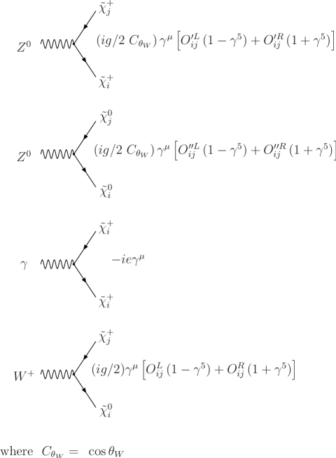
Refer to caption
Figure 19: Feynman rules for interaction of neutral and charged gauge boson with charginos and neutralinos.

B.2 Chargino-neutralino - W±superscript𝑊plus-or-minusW^{\pm}

Now in terms of physical chargino and neutralino states the relevant interaction term is

Wχ~±χ~0=Wχ~+χ~0+W+χ~χ~0,subscriptsuperscript𝑊minus-or-plussuperscript~𝜒plus-or-minussuperscript~𝜒0subscriptsuperscript𝑊superscript~𝜒superscript~𝜒0subscriptsuperscript𝑊superscript~𝜒superscript~𝜒0\mathcal{L}_{{W^{\mp}}{\tilde{\chi}^{\pm}}{\tilde{\chi}^{0}}}=\mathcal{L}_{{W^{-}}{\tilde{\chi}^{+}}{\tilde{\chi}^{0}}}+\mathcal{L}_{{W^{+}}{\tilde{\chi}^{-}}{\tilde{\chi}^{0}}}, (141)

where W+χ~χ~0subscriptsuperscript𝑊superscript~𝜒superscript~𝜒0\mathcal{L}_{{W^{+}}{\tilde{\chi}^{-}}{\tilde{\chi}^{0}}} is the hermitian conjugate of Wχ~+χ~0subscriptsuperscript𝑊superscript~𝜒superscript~𝜒0\mathcal{L}_{{W^{-}}{\tilde{\chi}^{+}}{\tilde{\chi}^{0}}} and

Wχ~+χ~0=gWμχ~¯i0γμ[OijLPL+OijRPR]χ~j+,subscriptsuperscript𝑊superscript~𝜒superscript~𝜒0𝑔subscriptsuperscript𝑊𝜇subscriptsuperscript¯~𝜒0𝑖superscript𝛾𝜇delimited-[]subscriptsuperscript𝑂𝐿𝑖𝑗subscript𝑃𝐿subscriptsuperscript𝑂𝑅𝑖𝑗subscript𝑃𝑅subscriptsuperscript~𝜒𝑗\displaystyle\mathcal{L}_{{W^{-}}{\tilde{\chi}^{+}}{\tilde{\chi}}^{0}}=gW^{-}_{\mu}\bar{\tilde{\chi}}^{0}_{i}\gamma^{\mu}\left[O^{L}_{ij}P_{L}+O^{R}_{ij}P_{R}\right]\tilde{\chi}^{+}_{j}, (142)

with

OijL=Ni2Vj112Ni4Vj2,subscriptsuperscript𝑂𝐿𝑖𝑗subscript𝑁𝑖2subscriptsuperscript𝑉𝑗112subscript𝑁𝑖4subscriptsuperscript𝑉𝑗2\displaystyle O^{L}_{ij}=N_{i2}V^{*}_{j1}-\frac{1}{\sqrt{2}}N_{i4}V^{*}_{j2},
OijR=Ni2Uj1+12Ni3Uj2+12Ni,k+7Uj,k+2,subscriptsuperscript𝑂𝑅𝑖𝑗subscriptsuperscript𝑁𝑖2subscript𝑈𝑗112subscriptsuperscript𝑁𝑖3subscript𝑈𝑗212subscriptsuperscript𝑁𝑖𝑘7subscript𝑈𝑗𝑘2\displaystyle O^{R}_{ij}=N^{*}_{i2}U_{j1}+\frac{1}{\sqrt{2}}N^{*}_{i3}U_{j2}+\frac{1}{\sqrt{2}}N^{*}_{i,k+7}U_{j,k+2},

where k=1,2,3𝑘123k=1,2,3.

The Feynman rules are shown in fig.19. The matrices OijLsubscriptsuperscript𝑂𝐿𝑖𝑗O^{\prime L}_{ij}, OijRsubscriptsuperscript𝑂𝑅𝑖𝑗O^{\prime R}_{ij}, Oij′′Lsubscriptsuperscript𝑂′′𝐿𝑖𝑗O^{\prime\prime L}_{ij}, Oij′′Rsubscriptsuperscript𝑂′′𝑅𝑖𝑗O^{\prime\prime R}_{ij} and OijLsubscriptsuperscript𝑂𝐿𝑖𝑗O^{L}_{ij}, OijRsubscriptsuperscript𝑂𝑅𝑖𝑗O^{R}_{ij} are defined by eq.(B.1) and eq.(B.2), respectively.

References