Age spreads in star forming regions?

Abstract

Rotation periods and projected equatorial velocities of pre-main-sequence (PMS) stars in star forming regions can be combined to give projected stellar radii. Assuming random axial orientation, a Monte-Carlo model is used to illustrate that distributions of projected stellar radii are very sensitive to ages and age dispersions between 1 and 10 Myr which, unlike age estimates from conventional Hertzsprung-Russell diagrams, are relatively immune to uncertainties due to extinction, variability, distance etc. Application of the technique to the Orion Nebula cluster reveals radius spreads of a factor of 2–3 (FWHM) at a given effective temperature. Modelling this dispersion as an age spread suggests that PMS stars in the ONC have an age range larger than the mean cluster age, that could be reasonably described by the age distribution deduced from the Hertzsprung-Russell diagram. These radius/age spreads are certainly large enough to invalidate the assumption of coevality when considering the evolution of PMS properties (rotation, disks etc.) from one young cluster to another.

1 Introduction

Does star formation take a long time, or is it all over on a dynamical free-fall timescale? This is a keenly debated question in star formation theory, with implications spanning topics as diverse as investigating early star/disk/planet evolution using populations in young star formation regions (SFRs) which are often assumed to be coeval, through to assessing overall star formation efficiency and the build up of galactic populations.

According to one paradigm, the collapse of molecular clouds is a quasi-static process slowed by magnetic pressure. The timescale for star formation is governed by ambipolar diffusion and could be $\simeq 10$ Myr (e.g. Tan, Krumholz & McKee 2006). Alternatively, on the basis of short deduced molecular cloud lifetimes, others argue that star formation is a rapid process, taking place in compressed filamentary structures on free-fall timescales $\leq 1$ Myr (e.g. Elmegreen 2007).

A crucial piece of evidence for star formation timescales is the presence (or not) of age spreads among stars in young SFRs. Low-mass pre-main-sequence (PMS) stars can be assigned model-dependent ages from their position in Hertzsprung-Russell (H-R) diagrams as they contract along Hayashi tracks. Using this technique several authors (e.g. Palla & Stahler 2000; Huff & Stahler 2006) claim star formation “accelerates” exponentially up to the present day, on timescales of $\simeq 10$ Myr. These apparent age spreads favour quasi-static, “slow” star formation. However, conventional H-R diagrams are severely affected by (i) intrinsic variability, (ii) extinction uncertainties, (iii) accretion luminosity, (iv) binarity, (v) distance dispersion – all of which can mimic age spreads where none exist (e.g. Hartmann 2001; Hillenbrand, Bauermeister & White 2008).

In this contribution I illustrate a technique to circumvent these difficulties using the rotational properties of PMS stars. This produces an alternative H-R diagram (radius versus temperature) that can be modelled to reconstruct a star formation history free from the problems above (e.g. see Jeffries 2007a,b).

2 Projected stellar radii

New wide-field surveys are finding rotation periods ($P$ in days) for hundreds of magnetically spotted PMS stars in SFRs. At the same time, it is now possible to obtain projected equatorial velocities ($v\sin i$ in km s^-1) for these stars from rotational line broadening using multi-object spectrographs such as FLAMES at the VLT and Hectoechelle at the MMT. Combining these measurements gives geometric estimates of radii, $R\sin i=0.02\,P\,v\sin i$ (in solar radii). The inclination angle, $i$, is unknown, but if it is assumed random (for which there is some evidence – e.g. Jackson & Jeffries in these proceedings – and no counter evidence) and the measurement uncertainties are understood, then distributions of $R\sin i$ can be Monte-Carlo modelled to estimate the true $R$ for any group of stars.

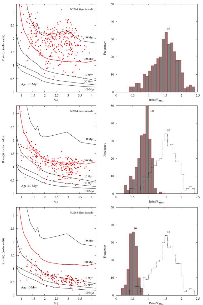
As an example of the technique’s power, in Fig. 1 I show a simulation of what could be achieved by observing projected equatorial velocities for 458 PMS objects with rotation periods in the young SFR NGC 2264 (from Lamm et al. 2004 and Makidon et al. 2004), with a 10% precision and a threshold for detection of $v\sin i\geq 15$ km s^-1 – which is routinely possible. The simulation assumes that rotation axes are randomly oriented but that objects with $i<30^{\circ}$ do not show rotational modulation. The left hand panels show the recovered $R\sin i$ values versus $V-I$ for coeval populations at several ages, where the Siess, Dufour & Forestini (2000, S00) isochrones are used to assign the intrinsic stellar radii. The right hand panels collapse this distribution to 1-dimensional form by normalising $R\sin i$ at each colour by the value of $R$ at 3 Myr.

With typical measurements, a set of 20 $R\sin i$ values can give $R$ to $\pm 5\%$. But at a given colour or $T_{\rm eff}$, $R$ is expected to change by a factor of three between 1 and 10 Myr! Hence the $R\sin i$ distribution is very sensitive to age differences and age dispersions in this range (see right panels of Fig. 1), but becomes less so at older ages. Any inferred ages and age spreads are of course model-dependent, but the radii are absolute. The technique is almost immune to problems associated with variability, binarity, extinction uncertainty and accretion luminosity. It is also distance-independent to boot!

Figure 1: A simulation of the expected $R\sin i$ values that would be obtained from a sample of 458 periodic PMS stars in the young SFR NGC 2264. The left hand panels show $R\sin i$ values versus colour assuming random rotation axis orientation and that only $v\sin i$ values $\geq 15$ km s^-1 are detectable. The right hand panels show the 1-dimensional collapsed distribution obtained by normalising by the expected radius at an age of 3 Myr. The simulations include typical measurement uncertainties in colour, $v\sin i$ and period. Each row shows how the distribution would look if the NGC 2264 stars were coeval and at ages of 1, 3 or 10 Myr. The solid lines are radius isochrones from Siess et al. (2000).

3 Results for the Orion Nebula Cluster

Figure 2: (Left) The measured normalised $R\sin i$ distribution for the ONC compared with a coeval model ($\sigma_{r}=0.0$). This model distribution is too narrow. Also shown is a model with a Gaussian spread ($\sigma_{r}=0.15$ dex) in $\log_{10}R$ which provides a much better fit. In both cases, the central age for the distribution is 1.78 Myr. (Right) The probability distribution for $\sigma_{r}$ using either the S00 or DAM97 isochrones. The 90% confidence region for the S00 isochrones is shown, but the result is almost identical for the DAM97 isochrones. This modelling implies a spread of a factor 2–3 (FWHM) in radius at a given $T_{\rm eff}$.

The first attempts to use this technique were made in the Orion Nebula Cluster (ONC). The results were described in detail by Jeffries (2007b) and are summarised here. The ONC is a young and populous SFR with a sample of 95 K- and M-stars that have measured rotation periods (Herbst et al. 2002), effective temperatures (Hillenbrand 1997) and $v\sin i$ (Rhode, Herbst & Mathieu 2001; Sicilia-Aguilar et al. 2005).

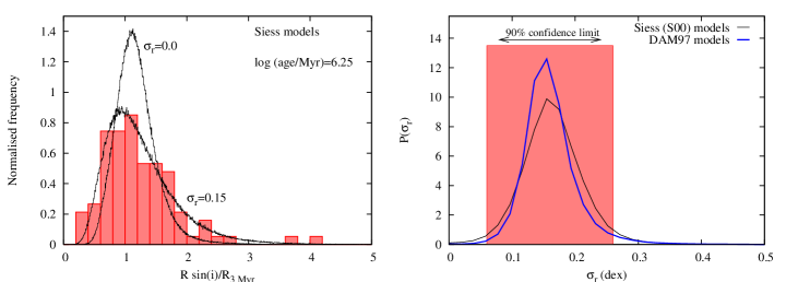
I calculated $R\sin i$ for these stars and then simulated the normalised (to $R_{\rm 3Myr}$) distributions using the Monte Carlo model which produced the simulations in Fig. 1. The models were tested against the observed data using the Kolmogorov-Smirnoff statistic on the cumulative distributions. The simulations are insensitive to the threshold $i$ below which it is assumed no rotational periodicity would be found, but are sensitive to the choice of radius isochrones. I ran models using the S00 and D’Antona & Mazzitelli (1997, DAM97) isochrones. Uncertainties in periods, $v\sin i$ and $T_{\rm eff}$ were taken from the sources cited above.

The first models I tried were coeval with the age as a free parameter. The best-fitting ages were 1.78 Myr and 0.76 Myr for the S00 and DAM97 isochrones, but both were rejected as good models at the $>95\%$ level (see Fig. 2). New models were generated by allowing the radius to spread around a single coeval value. The spread was characterised by a Gaussian $\sigma_{r}$ in $\log_{10}R$. These generated good fits with central ages very similar to the previous coeval model, but with $\sigma_{r}\simeq(0.15\pm 0.08)$ dex (90% confidence interval) for both sets of isochrones (see Fig. 2). This implies linear radius spreads of a factor of 2–3 (FWHM) at a given $T_{\rm eff}$.

Rather than a simple radius spread it is natural to interpret the results in terms of an age spread. I fitted two types of analytic age spread: a Gaussian spread ($\sigma_{a}$) in $\log_{10}$ age about a central value

$$f(\log_{10}{\rm age})=N_{0}\exp\left(\frac{-(\log_{10}{\rm age}-\log_{10}{\rm central\ age})^{2}}{2\sigma_{a}^{2}}\right)\,;$$

or an exponentially accelerating star forming rate with timescale $\lambda_{a}$ and an abrupt cut-off (or zero-point) age

$$f({\rm age})=N_{0}\exp\left(-\frac{{\rm age}}{\lambda_{a}}\right)\ \ \ \ {\rm for\ age}>{\rm zeropoint\ age}\,.$$

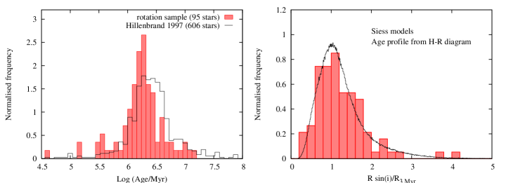
Finally, I modelled the $R\sin i$ distribution by assuming that the stars had the age distribution implied by their positions in the H-R diagram (assuming an ONC distance of 392 pc – Jeffries 2007a).

Figure 3: Relative probability distributions of a good fit in the cases of a Gaussian distribution in $\log_{10}$age (top row, with free parameters of a central age and dispersion $\sigma_{a}$ in dex) and an exponentially accelerating star formation rate (bottom row, with free parameters of a timescale $\lambda_{a}$ and a zero-point cut-off age. For each model we show the results using either the S00 or DAM97 isochrones. The contours enclose 68%, 90% and 99% of the probability.

Figure 4: (Left) Normalised age distribution of ONC PMS stars estimated from the H-R diagram and S00 isochrones. I show normalised distributions for the rotation sample and the full sample of Hillenbrand (1997). The rotation sample is missing some of the “oldest” stars. (Right) The $R\sin i$ distribution modelled using the age distribution for the rotation sample in the left-hand panel is a reasonable fit to the observed $R\sin i$ distribution.

There are three main results, summarised below.

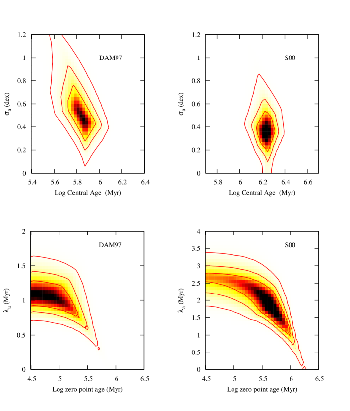
1. Both classes of model require an age spread ($\sigma_{a}>0$, $\lambda_{a}>0$ – see Fig.3). For the Gaussian model the best fitting dispersion $\sigma_{a}\simeq 0.4$ dex is independent of isochrone choice, but with model-dependent central ages similar to those given by the coeval models. The exponential model has a best-fitting $\lambda_{a}\simeq 1.1$ Myr for the DAM97 isochrones and $\lambda_{a}\simeq 1.9$ Myr for the S00 isochrones.

2. The data are incapable of distinguishing between the exponentially accelerating model or the Gaussian spread in $\log_{10}$age.

3. Modelling the $R\sin i$ distribution using the ages derived from the H-R diagram (see Fig. 4) gives a reasonable fit for both sets of isochrones.

4 Discussion

Although the absolute ages and age dispersions derived with this technique are to some extent model-dependent, the absolute radii and radius dispersion are geometric estimates. We conclude that there is very strong evidence for spreads amounting to factors of 2-3 (FWHM) in radius at a given $T_{\rm eff}$ in PMS stars of the ONC. As PMS tracks are close-to-vertical in the H-R diagram for low-mass stars, this implies order-of-magnitude spreads in moment of inertia – a fact that cannot be ignored when considering the angular momentum evolution of PMS stars in SFRs.

Whether these radius spreads represent real age spreads is a moot point. It is possible that differing accretion histories could lead to luminosity/radius differences for coeval stars of similar present-day $T_{\rm eff}$. However, according to current, non-accreting models, the data imply age spreads in the ONC that are larger than its mean age ($>2$ Myr for the S00 models), consistent with age spreads judged from its conventional H-R diagram, and certainly large enough to compromise any coeval assumption. In addition, the spreads we have found may actually be underestimates. The rotation sample in the ONC is clearly biased against the faintest (possibly oldest?) stars (see Fig. 4). We cannot comment on whether age spreads as large as 10 Myr are likely until these low-luminosity outliers in the ONC have their periods and projected rotation velocities measured.

References

- [D’Antona & Mazzitelli (1997)] D’Antona, F. & Mazzitelli, I. 1997, MemSAI, 68, 807
- [Elmegreen (2007)] Elmegreen, B. G. 2007, ApJ, 668, 1064
- [Hartmann (2001)] Hartmann, L. W. 2001, AJ, 121, 1030
- [Herbst et al. (2002)] Herbst, W., Bailer-Jones, C. A. L., Mundt, R., Meisenheimer, K. & Wackermann, R. 2002, A&A, 396, 513
- [Hillenbrand (1997)] Hillenbrand, L. A. 1997, AJ, 113, 1733
- [Hillenbrand, Bauermeister & White (2008)] Hillenbrand, L. A., Bauermeister, A. & White, R. J. 2008, in G. van Belle (ed.), 14th Cambridge Workshop on Cool Stars, Stellar Systems and the Sun, (San Francisco: Astronomical Society of the Pacific), p.200
- [Huff & Stahler (2006)] Huff, E. M. & Stahler, S. W. 2006, ApJ, 644, 355
- [Jeffries (2007a)] Jeffries, R. D. 2007a, MNRAS, 376, 1109
- [Jeffries (2007b)] Jeffries, R. D. 2007b, MNRAS, 381, 1169
- [Lamm et al. 2004] Lamm, M., Bailer-Jones, C. A. L., Mundt, R. & Herbst, W. 2005, A&A, 417, 557
- [Makidon et al. 2004] Makidon, R. B., Rebull, L. M., Strom, S. E., Adams, M. T. & Patten, B. M. 2004, AJ, 127, 2228
- [Palla & Stahler (2000)] Palla, F. & Stahler, S. W. 2000, ApJ 540, 255
- [Rhode et al. (2001)] Rhode, K. L., Herbst, W. & Mathieu, R. D. 2001, AJ 122, 3258
- [Sicilia-Aguilar et al. (2005)] Sicilia-Aguilar, A., Hartmann, L. W., Hernández, J., Briceño, C. & Calvet, N. 2005, AJ 130, 188
- [Siess, Dufour & Forestini (2000)] Siess, L., Dufour, E. & Forestini, M. 2000, A&A 358, 593
- [Tan, Krumholz & McKee (2006)] Tan, J. C., Krumholz, M. R. & McKee, C. F. 2006, ApJ, 641, L121