The homogenization of orthorhombic piezoelectric composites by the strong–property–fluctuation theory

Andrew J. Duncan111Corresponding author. E–mail: Andrew.Duncan@ed.ac.uk., Tom G. Mackay222E–mail: T.Mackay@ed.ac.uk.
School of Mathematics and Maxwell Institute for Mathematical Sciences
University of Edinburgh, Edinburgh EH9 3JZ, UK

Akhlesh Lakhtakia333E–mail: akhlesh@psu.edu
NanoMM — Nanoengineered Metamaterials Group
Department of Engineering Science and Mechanics
Pennsylvania State University, University Park, PA 16802–6812, USA

Abstract

The linear strong–property–fluctuation theory (SPFT) was developed in order to estimate the constitutive parameters of certain homogenized composite materials (HCMs) in the long–wavelength regime. The component materials of the HCM were generally orthorhombic mm2𝑚𝑚2mm2 piezoelectric materials, which were randomly distributed as oriented ellipsoidal particles. At the second–order level of approximation, wherein a two–point correlation function and its associated correlation length characterize the component material distributions, the SPFT estimates of the HCM constitutive parameters were expressed in terms of numerically–tractable two–dimensional integrals. Representative numerical calculations revealed that: (i) the lowest–order SPFT estimates are qualitatively similar to those provided by the corresponding Mori–Tanaka homogenization formalism, but differences between the two estimates become more pronounced as the component particles become more eccentric in shape; and (ii) the second–order SPFT estimate provides a significant correction to the lowest–order estimate, which reflects dissipative losses due to scattering.

Keywords: Homogenization, strong–property–fluctuation theory, metamaterials, Mori–Tanaka formalism, orthorhombic piezoelectric.

1 Introduction

Since piezoelectric materials can convert electrical energy to mechanical energy, and vice versa, they are of considerable technological importance. However, bulk piezoelectric materials commonly exhibit physical properties which render them unsuitable for particular applications. For example, certain ceramics exhibit strong piezoelectric properties but their weight, malleability and acoustic impedance are not suitable for transducer applications [1]. Accordingly, composite piezoelectric materials are often more technologically attractive [2]; and these can be found in a host of applications such as in transducers, sensors, actuators and energy harvesting devices, for example [3, 4]. Furthermore, the recent proliferation of multifunctional metamaterials [5] — which often take the form of homogenized composite materials (HCMs), exhibiting exotic constitutive properties [6] — presents interesting possibilities for piezoelectric HCMs.

While the estimation of elastodynamic or electromagnetic constitutive parameters of HCMs is a challenging task, especially for anisotropic HCMs, the estimation of constitutive parameters of piezoelectric HCMs is more challenging due to the coupling of elastodynamic and electromagnetic fields. Numerous homogenization formalisms have been proposed for piezoelectric HCMs, many of which build upon Eshelby’s landmark description of the elastodynamic response of a single ellipsoidal particle immersed in an infinite homogeneous medium [7, 8]. For example, the Mori–Tanaka [9, 10, 11], self–consistent and differential approaches [12] — and combinations of these [13] — feature prominently in the literature. In the following we present a fundamentally different approach to estimating the constitutive properties of piezoelectric HCMs, based on the strong–property–fluctuation theory (SPFT). A key feature of the SPFT homogenization approach — which distinguishes it from other more conventional approaches — is the accommodation of higher–order characterizations of the distributional statistics of the HCM’s component materials.

The origins of the SPFT lie in wave propagation studies for continuously random mediums [14]. It was later adapted to estimate the electromagnetic [15, 16, 17], acoustic [18] and elastodynamic [19] constitutive parameters of HCMs. Within the SPFT, the estimation the HCMs constitutive parameters arises by successive refinements to the constitutive parameters of a homogeneous comparison medium. Iterations are expressed in terms of correlation functions describing the spatial distributions of the component materials. In principle, correlation functions of arbitrarily high–order may be incorporated; but, in practice, the SPFT is most often implemented at the second–order level of approximation, wherein a two–point correlation function and its associated correlation length characterize the component material distributions.

We establish here the linear, second–order SPFT appropriate to orthorhombic mm2𝑚𝑚2mm2 piezoelectric HCMs, arising from component materials which are randomly distributed as oriented ellipsoidal particles. The theoretical development builds upon the corresponding development of the orthotropic elastodynamic SPFT [19, 20]. A representative numerical example is used to illustrate the theory, and results are compared with those from the well–established Mori–Tanaka formalism.

2 Theory

2.1 Preliminaries

In the following, we consider piezoelectric materials described by constitutive relations of the form [21, 22]

σab=CabmnSmnenabEnDa=eamnSmn+ϵanEn},casessubscript𝜎𝑎𝑏subscript𝐶𝑎𝑏𝑚𝑛subscript𝑆𝑚𝑛subscript𝑒𝑛𝑎𝑏subscript𝐸𝑛subscript𝐷𝑎subscript𝑒𝑎𝑚𝑛subscript𝑆𝑚𝑛subscriptitalic-ϵ𝑎𝑛subscript𝐸𝑛\left.\begin{array}[]{l}\sigma_{ab}=C_{abmn}S_{mn}-e_{nab}E_{n}\\ D_{a}=e_{amn}S_{mn}+\epsilon_{an}E_{n}\end{array}\right\}, (1)

wherein the elastic strain Smnsubscript𝑆𝑚𝑛S_{mn} and the electric field Ensubscript𝐸𝑛E_{n} are taken as independent variables, which are related to the stress σabsubscript𝜎𝑎𝑏\sigma_{ab} and dielectric displacement Dasubscript𝐷𝑎D_{a} via the elastic stiffness tensor Cabmnsubscript𝐶𝑎𝑏𝑚𝑛C_{abmn} (measured in a constant electric field), the piezoelectric tensor enabsubscript𝑒𝑛𝑎𝑏e_{nab} (measured at a constant strain or electric field), and the dielectric tensor ϵansubscriptitalic-ϵ𝑎𝑛\epsilon_{an} (measured at a constant strain). Here, and hereafter, tensors are represented in plain font and lowercase tensor indexes range from 1 to 3, with a repeated index implying summation.

We develop the SPFT in the frequency domain. Accordingly the complex–valued representations of the stress, strain and electromagnetic fields have an implicit exp(iωt)𝑖𝜔𝑡\exp\left(-i\omega t\right) dependency on time t𝑡t, with ω𝜔\omega being the angular frequency and i=1𝑖1i=\sqrt{-1}. The possibility of dissipative behaviour is thereby accommodated via the imaginary parts of complex–valued constitutive parameters.

The constitutive relations (1) are more conveniently expressed in the symbolic form

σ˘aB=C˘aBMnS˘Mn,subscript˘𝜎𝑎𝐵subscript˘𝐶𝑎𝐵𝑀𝑛subscript˘𝑆𝑀𝑛\breve{\sigma}_{aB}=\breve{C}_{aBMn}\breve{S}_{Mn}, (2)

where the extended stress symbol

σ˘aB={σab,B=b=1,2,3Da,B=4,subscript˘𝜎𝑎𝐵casessubscript𝜎𝑎𝑏missing-subexpressionformulae-sequence𝐵𝑏123subscript𝐷𝑎missing-subexpression𝐵4\breve{\sigma}_{aB}=\left\{\begin{array}[]{lcr}\sigma_{ab},&&B=b=1,2,3\\ D_{a},&&B=4\\ \end{array}\right., (3)

the extended stiffness symbol

C˘aBMn={Cabmn,B=b=1,2,3;M=m=1,2,3enab,B=b=1,2,3;M=4eamn,B=4;M=m=1,2,3ϵan,B,M=4,subscript˘𝐶𝑎𝐵𝑀𝑛casessubscript𝐶𝑎𝑏𝑚𝑛missing-subexpressionformulae-sequence𝐵𝑏123𝑀𝑚123subscript𝑒𝑛𝑎𝑏missing-subexpressionformulae-sequence𝐵𝑏123𝑀4subscript𝑒𝑎𝑚𝑛missing-subexpressionformulae-sequenceformulae-sequence𝐵4𝑀𝑚123subscriptitalic-ϵ𝑎𝑛missing-subexpression𝐵𝑀4\breve{C}_{aBMn}=\left\{\begin{array}[]{lcr}C_{abmn},&&B=b=1,2,3;\>M=m=1,2,3\\ e_{nab},&&B=b=1,2,3;\>M=4\\ -e_{amn},&&B=4;\>M=m=1,2,3\\ \epsilon_{an},&&B,M=4\\ \end{array}\right., (4)

and the extended strain symbol

S˘Mn={Smn,M=m=1,2,3En,M=4.subscript˘𝑆𝑀𝑛casessubscript𝑆𝑚𝑛missing-subexpressionformulae-sequence𝑀𝑚123subscript𝐸𝑛missing-subexpression𝑀4\breve{S}_{Mn}=\left\{\begin{array}[]{lcr}S_{mn},&&M=m=1,2,3\\ E_{n},&&M=4\\ \end{array}\right.. (5)

Here, and hereafter, uppercase indexes range from 1 to 4. Note that the extended quantities defined in eqs. (3), (4) and (5) are not tensors — these are simply symbols which are introduced to allow a compact representation of the piezoelectric constitutive relations [10].

In developing the SPFT appropriate to piezoelectric HCMs, it is expedient to express the constitutive relations (2) in matrix–vector form as

𝝈˘=𝐂¯¯˘𝐒˘,bold-˘𝝈˘¯¯𝐂˘𝐒\mbox{\boldmath$\breve{{\bf\sigma}}$}=\breve{\underline{\underline{\bf C}}}\cdot\breve{{\bf S}}, (6)

wherein 𝝈˘bold-˘𝝈\breve{{\bf\sigma}} and 𝐒˘˘𝐒\breve{{\bf S}} are column 12–vectors representing the extended stress and extended strain symbols, respectively, and 𝐂¯¯˘˘¯¯𝐂\breve{\underline{\underline{\bf C}}} is a 12×\times12 matrix which represents the extended stiffness symbol. Here, and hereafter, matrixes are denoted by double underlining and bold font, whereas vectors are in bold font with no underlining. For use later on, we note that the pq𝑝𝑞pqth entry of a matrix 𝐀¯¯¯¯𝐀\underline{\underline{\bf A}} is written as [𝐀¯¯]pqsubscriptdelimited-[]¯¯𝐀𝑝𝑞\left[\,\underline{\underline{\bf A}}\,\right]_{pq}, while the p𝑝pth entry of a vector 𝐛𝐛{\bf b} is written as [𝐛]psubscriptdelimited-[]𝐛𝑝\left[\,{\bf b}\,\right]_{p}. Accordingly, the matrix entry [𝐀¯¯𝐁¯¯]pr=[𝐀¯¯]pq[𝐁¯¯]qrsubscriptdelimited-[]¯¯𝐀¯¯𝐁𝑝𝑟subscriptdelimited-[]¯¯𝐀𝑝𝑞subscriptdelimited-[]¯¯𝐁𝑞𝑟\big{[}\,\underline{\underline{\bf A}}\cdot\underline{\underline{\bf B}}\,\big{]}_{pr}=\big{[}\,\underline{\underline{\bf A}}\,\big{]}_{pq}\big{[}\,\underline{\underline{\bf B}}\,\big{]}_{qr}, the vector entry [𝐀¯¯𝐛]p=[𝐀¯¯]pq[𝐛]qsubscriptdelimited-[]¯¯𝐀𝐛𝑝subscriptdelimited-[]¯¯𝐀𝑝𝑞subscriptdelimited-[]𝐛𝑞\big{[}\,\underline{\underline{\bf A}}\cdot{\bf b}\big{]}_{p}=\big{[}\,\underline{\underline{\bf A}}\,\big{]}_{pq}\big{[}{\bf b}\big{]}_{q}, and the scalar 𝐚𝐛=[𝐚]p[𝐛]p𝐚𝐛subscriptdelimited-[]𝐚𝑝subscriptdelimited-[]𝐛𝑝{\bf a}\cdot{\bf b}=\left[{\bf a}\right]_{p}\left[{\bf b}\right]_{p}. The adjoint, determinant, inverse, trace and transpose of a matrix 𝐀¯¯¯¯𝐀\underline{\underline{\bf A}} are denoted by adj(𝐀¯¯)adj¯¯𝐀\mbox{adj}\left(\,\underline{\underline{\bf A}}\,\right), det(𝐀¯¯)det¯¯𝐀\mbox{det}\left(\,\underline{\underline{\bf A}}\,\right), 𝐀¯¯1superscript¯¯𝐀1\underline{\underline{\bf A}}^{-1}, tr(𝐀¯¯)tr¯¯𝐀\mbox{tr}\left(\,\underline{\underline{\bf A}}\,\right) and 𝐀¯¯Tsuperscript¯¯𝐀𝑇\underline{\underline{\bf A}}^{T}, respectively. The n×n𝑛𝑛n\times n null matrix is written as 𝟎¯¯n×nsubscript¯¯0𝑛𝑛\underline{\underline{\bf 0}}_{\,n\times n}.

Our concern in this article is with orthorhombic mm2𝑚𝑚2mm2 piezoelectric materials [21, 22]. For this symmetry class, the extended stiffness matrix has the block matrix form

𝐂¯¯˘=(𝐂¯¯𝐞¯¯T𝐞¯¯ϵ¯¯),˘¯¯𝐂¯¯𝐂superscript¯¯𝐞𝑇¯¯𝐞bold-¯bold-¯bold-italic-ϵ\breve{\underline{\underline{\bf C}}}=\left(\begin{array}[]{cc}\underline{\underline{\bf C}}&-\underline{\underline{\bf e}}^{T}\vspace{8pt}\\ \underline{\underline{\bf e}}&\mbox{\boldmath$\underline{\underline{\bf\epsilon}}$}\end{array}\right), (7)

where the 9×\times9 stiffness matrix 𝐂¯¯¯¯𝐂\underline{\underline{\bf C}} may be expressed as

𝐂¯¯=(𝐂¯¯a𝟎¯¯ 3×3𝟎¯¯ 3×3𝟎¯¯ 3×3𝐂¯¯b𝐂¯¯b𝟎¯¯ 3×3𝐂¯¯b𝐂¯¯b),¯¯𝐂subscript¯¯𝐂𝑎subscript¯¯033subscript¯¯033subscript¯¯033subscript¯¯𝐂𝑏subscript¯¯𝐂𝑏subscript¯¯033subscript¯¯𝐂𝑏subscript¯¯𝐂𝑏\underline{\underline{\bf C}}=\left(\begin{array}[]{ccc}\underline{\underline{\bf C}}_{\,a}&\underline{\underline{\bf 0}}_{\,3\times 3}&\underline{\underline{\bf 0}}_{\,3\times 3}\\ \underline{\underline{\bf 0}}_{\,3\times 3}&\underline{\underline{\bf C}}_{\,b}&\underline{\underline{\bf C}}_{\,b}\\ \underline{\underline{\bf 0}}_{\,3\times 3}&\underline{\underline{\bf C}}_{\,b}&\underline{\underline{\bf C}}_{\,b}\end{array}\right), (8)

with the 3×\times3 symmetric matrix components

𝐂¯¯a=(C11C12C13C12C22C23C13C23C33),𝐂¯¯b=(C44000C55000C66);formulae-sequencesubscript¯¯𝐂𝑎subscript𝐶11subscript𝐶12subscript𝐶13subscript𝐶12subscript𝐶22subscript𝐶23subscript𝐶13subscript𝐶23subscript𝐶33subscript¯¯𝐂𝑏subscript𝐶44000subscript𝐶55000subscript𝐶66\underline{\underline{\bf C}}_{\,a}=\left(\begin{array}[]{ccc}C_{11}&C_{12}&C_{13}\\ C_{12}&C_{22}&C_{23}\\ C_{13}&C_{23}&C_{33}\end{array}\right),\qquad\underline{\underline{\bf C}}_{\,b}=\left(\begin{array}[]{ccc}C_{44}&0&0\\ 0&C_{55}&0\\ 0&0&C_{66}\end{array}\right); (9)

while the 9×\times3 piezoelectric matrix 𝐞¯¯¯¯𝐞\underline{\underline{\bf e}} may be expressed as

𝐞¯¯=(0000e1500e150000e2400e2400e31e32e33000000)¯¯𝐞0000subscript𝑒1500subscript𝑒150000subscript𝑒2400subscript𝑒2400subscript𝑒31subscript𝑒32subscript𝑒33000000\underline{\underline{\bf e}}=\left(\begin{array}[]{ccccccccc}0&0&0&0&e_{15}&0&0&e_{15}&0\\ 0&0&0&e_{24}&0&0&e_{24}&0&0\\ e_{31}&e_{32}&e_{33}&0&0&0&0&0&0\end{array}\right) (10)

and the 3×\times3 dielectric matrix ϵ¯¯bold-¯bold-¯bold-italic-ϵ\underline{\underline{\bf\epsilon}} as

ϵ¯¯=(ϵ11000ϵ22000ϵ33).bold-¯bold-¯bold-italic-ϵsubscriptitalic-ϵ11000subscriptitalic-ϵ22000subscriptitalic-ϵ33\mbox{\boldmath$\underline{\underline{\bf\epsilon}}$}=\left(\begin{array}[]{ccc}\epsilon_{11}&0&0\\ 0&\epsilon_{22}&0\\ 0&0&\epsilon_{33}\end{array}\right). (11)

The correspondence between the tensor/extended symbol representation and the matrix–vector representation is described in Appendix A.

In an analogous fashion, the material density ρ𝜌\rho may be represented via the extended density symbol

ρ˘BM={ρ,B=M=1,2,30,otherwise,subscript˘𝜌𝐵𝑀cases𝜌missing-subexpressionformulae-sequence𝐵𝑀1230missing-subexpressionotherwise\breve{\rho}_{BM}=\left\{\begin{array}[]{lcr}\rho,&&B=M=1,2,3\\ 0,&&\textrm{otherwise}\\ \end{array}\right., (12)

which has the 4×\times4 extended matrix counterpart 𝝆¯˘¯bold-¯bold-¯bold-˘𝝆\underline{\underline{\bf\breve{\rho}}} with entries

[𝝆¯˘¯]MP=ρ˘MP.subscriptdelimited-[]bold-¯bold-¯bold-˘𝝆𝑀𝑃subscript˘𝜌𝑀𝑃\left[\,\mbox{\boldmath$\underline{\underline{\bf\breve{\rho}}}$}\,\right]_{MP}=\breve{\rho}_{MP}. (13)

2.2 Component materials

We consider the homogenization of a composite comprising two component materials, labelled as component material ‘1’ and component material ‘2’. In general, both components are homogeneous, orthorhombic mm2𝑚𝑚2mm2 piezoelectric materials, characterized by the stiffness tensors Cabmn()subscriptsuperscript𝐶𝑎𝑏𝑚𝑛C^{(\ell)}_{abmn}, piezoelectric tensors enab()subscriptsuperscript𝑒𝑛𝑎𝑏e^{(\ell)}_{nab}, dielectric tensors ϵan()subscriptsuperscriptitalic-ϵ𝑎𝑛\epsilon^{(\ell)}_{an} and densities ρ()superscript𝜌\rho^{(\ell)} (=1,2)12(\ell=1,2). In conformity with the notational practices introduced in §2.1, the component materials are also described by the extended stiffness symbols C˘aBMn()subscriptsuperscript˘𝐶𝑎𝐵𝑀𝑛\breve{C}^{(\ell)}_{aBMn} (and their 12×\times12 matrix equivalents 𝐂¯¯˘()superscript˘¯¯𝐂\breve{\underline{\underline{\bf C}}}^{(\ell)}) and extended density symbols ρ˘BM()subscriptsuperscript˘𝜌𝐵𝑀\breve{\rho}^{(\ell)}_{BM} (and their 4×\times4 matrix equivalents 𝝆¯˘¯()superscriptbold-¯bold-¯bold-˘𝝆\mbox{\boldmath$\underline{\underline{\bf\breve{\rho}}}$}^{(\ell)}).

The component materials are randomly distributed as identically–oriented, conformal, ellipsoidal particles. The principal axes of the ellipsoidal particles are aligned with the Cartesian axes. Thus, the surface of each ellipsoidal particle may be parameterized by the vector

𝐫(e)=η𝐔¯¯𝐫^,superscript𝐫𝑒𝜂¯¯𝐔^𝐫{\bf r}^{(e)}=\eta\underline{\underline{\bf U}}\cdot\hat{{\bf r}}, (14)

where η𝜂\eta is a linear measure of size, 𝐫^^𝐫\hat{{\bf r}} is the radial unit vector and the diagonal shape matrix

𝐔¯¯=1abc3(a000b000c),(a,b,c+).¯¯𝐔13𝑎𝑏𝑐𝑎000𝑏000𝑐𝑎𝑏𝑐superscript\underline{\underline{\bf U}}=\frac{1}{\sqrt[3]{abc}}\left(\begin{array}[]{ccc}a&0&0\\ 0&b&0\\ 0&0&c\\ \end{array}\right),\qquad\qquad(a,b,c\in\mathbb{R}^{+}). (15)

Let V𝑉V denote the space occupied by the composite material. Then V=V(1)V(2)𝑉superscript𝑉1superscript𝑉2V=V^{(1)}\cup V^{(2)} where V(1)superscript𝑉1V^{(1)} and V(2)superscript𝑉2V^{(2)} contain the two component materials labelled as ‘1’ and ‘2’, respectively, and V(1)V(2)=superscript𝑉1superscript𝑉2V^{(1)}\cap V^{(2)}=\emptyset. The distributional statistics of the component materials are described in terms of moments of the characteristic functions

Φ()(𝐫)={1,𝐫V(),(=1,2).0,𝐫V(),superscriptΦ𝐫cases1𝐫superscript𝑉missing-subexpression120𝐫superscript𝑉\Phi^{(\ell)}({\bf r})=\left\{\begin{array}[]{ll}1,&\qquad{\bf r}\in V^{(\ell)},\\ &\qquad\qquad\qquad\qquad\qquad\qquad(\ell=1,2).\\ 0,&\qquad{\bf r}\not\in V^{(\ell)},\end{array}\right. (16)

The first statistical moment of Φ()superscriptΦ\Phi^{(\ell)}, i.e.,

Φ()(𝐫)=f(),(=1,2),delimited-⟨⟩superscriptΦ𝐫superscript𝑓12\langle\,\Phi^{(\ell)}({\bf r})\,\rangle=f^{(\ell)},\qquad\qquad\left(\ell=1,2\right), (17)

delivers the volume fraction of component material \ell, which is subject to the constraint =12f()=1subscriptsuperscript21superscript𝑓1\displaystyle{\sum^{2}_{\ell=1}f^{(\ell)}=1}. The second statistical moment of Φ()superscriptΦ\Phi^{(\ell)} constitutes a two–point covariance function. Investigations involving the electromagnetic SPFT have demonstrated that the specific form of the covariance function has only a minor influence on estimates of HCM constitutive parameters, for a range of physically–plausible covariance functions [25]. Here we adopt the physically–motivated form [26]

Φ()(𝐫)Φ()(𝐫)={Φ()(𝐫)Φ()(𝐫),|U¯¯1(𝐫𝐫)|>LΦ()(𝐫),|U¯¯1(𝐫𝐫)|L,delimited-⟨⟩superscriptΦ𝐫superscriptΦsuperscript𝐫casesdelimited-⟨⟩superscriptΦ𝐫delimited-⟨⟩superscriptΦsuperscript𝐫missing-subexpressionsuperscript¯¯𝑈1𝐫superscript𝐫𝐿missing-subexpressionmissing-subexpressionmissing-subexpressiondelimited-⟨⟩superscriptΦ𝐫missing-subexpressionsuperscript¯¯𝑈1𝐫superscript𝐫𝐿\langle\,\Phi^{(\ell)}({\bf r})\,\Phi^{(\ell)}({\bf r}^{\prime})\,\rangle=\left\{\begin{array}[]{lll}\langle\,\Phi^{(\ell)}({\bf r})\,\rangle\langle\Phi^{(\ell)}({\bf r}^{\prime})\,\rangle\,,&&\hskip 28.45274pt|\,\underline{\underline{U}}^{-1}\cdot\left({\bf r}-{\bf r}^{\prime}\right)|>L\\ &&\\ \langle\,\Phi^{(\ell)}({\bf r})\,\rangle\,,&&\hskip 28.45274pt|\,\underline{\underline{U}}^{-1}\cdot\left({\bf r}-{\bf r}^{\prime}\right)|\leq L\end{array}\right., (18)

which has been widely used in electromagnetic and elastodynamic SPFT studies. The correlation length L𝐿L in eq. (18) is required to be much smaller than the associated piezoelectric wavelengths, but larger than the particle size parameter η𝜂\eta.

2.3 Comparison material

A homogeneous comparison material provides the initial ansatz for an iterative procedure that delivers a succession of SPFT estimates of the HCM constitutive parameters [19]. Accordingly, the comparison material represents the lowest–order SPFT estimate of the HCM. In consonance with the component materials, the comparison material is an orthorhombic mm2𝑚𝑚2mm2 piezoelectric material, in general. The piezoelectric constitutive properties of this orthorhombic comparison material (OCM) are encapsulated by its extended stiffness symbol C˘lMPq(ocm)subscriptsuperscript˘𝐶𝑜𝑐𝑚𝑙𝑀𝑃𝑞\breve{C}^{(ocm)}_{lMPq} (and its 12×\times12 matrix equivalent 𝐂¯¯˘(ocm)superscript˘¯¯𝐂𝑜𝑐𝑚\breve{\underline{\underline{\bf C}}}^{(ocm)}) and extended density symbol ρ˘MP(ocm)superscriptsubscript˘𝜌𝑀𝑃𝑜𝑐𝑚\breve{\rho}_{MP}^{(ocm)} (and its 4×\times4 matrix equivalent 𝝆¯˘¯(ocm)superscriptbold-¯bold-¯bold-˘𝝆𝑜𝑐𝑚\mbox{\boldmath$\underline{\underline{\bf\breve{\rho}}}$}^{(ocm)}).

In order to establish the spectral Green function for the OCM — which is a key element in the SPFT formulation — we first consider the corresponding extended equation of motion. This may be written in the frequency domain as [27]

C˘lMPq(ocm)lqu˘P+ω2u˘M=F˘M,subscriptsuperscript˘𝐶𝑜𝑐𝑚𝑙𝑀𝑃𝑞subscript𝑙subscript𝑞subscript˘𝑢𝑃superscript𝜔2subscript˘𝑢𝑀subscript˘𝐹𝑀\breve{C}^{(ocm)}_{lMPq}\partial_{l}\partial_{q}\breve{u}_{P}+\omega^{2}\breve{u}_{M}=-\breve{F}_{M}, (19)

where the extended displacement

u˘M={um,M=m=1,2,3Φ,P=4subscript˘𝑢𝑀casessubscript𝑢𝑚formulae-sequence𝑀𝑚123Φ𝑃4\breve{u}_{M}=\left\{\begin{array}[]{lr}u_{m},&M=m=1,2,3\\ \Phi,&P=4\end{array}\right. (20)

combines the displacement umsubscript𝑢𝑚u_{m} and electric scalar potential ΦΦ\Phi, and the extended body force

F˘M={Fm,M=m=1,2,3q,M=4subscript˘𝐹𝑀casessubscript𝐹𝑚formulae-sequence𝑀𝑚123𝑞𝑀4\breve{F}_{M}=\left\{\begin{array}[]{lr}F_{m},&M=m=1,2,3\\ -q,&M=4\end{array}\right. (21)

combines the body force Fmsubscript𝐹𝑚F_{m} and the electric charge q𝑞q. Accordingly, the sought after spectral Green function for the OCM emerges as the 4×\times4 matrix

𝐆¯¯(ocm)(𝐤)=[k2𝐚¯¯(𝐤^)ω2𝝆¯˘¯(ocm)]1,superscript¯¯𝐆𝑜𝑐𝑚𝐤superscriptdelimited-[]superscript𝑘2¯¯𝐚^𝐤superscript𝜔2superscriptbold-¯bold-¯bold-˘𝝆𝑜𝑐𝑚1\underline{\underline{\bf G}}^{(ocm)}({\bf k})=\big{[}k^{2}\underline{\underline{\bf a}}({\bf\hat{k}})-\omega^{2}\mbox{\boldmath$\underline{\underline{\bf\breve{\rho}}}$}^{(ocm)}\;\big{]}^{-1}, (22)

where the 4×\times4 matrix 𝐚¯¯(𝐤^)¯¯𝐚^𝐤\underline{\underline{\bf a}}({\bf\hat{k}}) has entries

[𝐚¯¯(𝐤^)]MP=ksC˘sMPq(ocm)kqk2.subscriptdelimited-[]¯¯𝐚^𝐤𝑀𝑃subscript𝑘𝑠superscriptsubscript˘𝐶𝑠𝑀𝑃𝑞𝑜𝑐𝑚subscript𝑘𝑞superscript𝑘2\left[\underline{\underline{\bf a}}({\bf\hat{k}})\right]_{MP}=\displaystyle{\frac{k_{s}\breve{C}_{sMPq}^{(ocm)}k_{q}}{k^{2}}}. (23)

Herein, 𝐤=k𝐤^𝐤𝑘^𝐤{\bf k}=k{\bf\hat{k}} (k1,k2,k3)absentsubscript𝑘1subscript𝑘2subscript𝑘3\equiv\left(k_{1},k_{2},k_{3}\right) with 𝐤^=(sinθcosϕ{\bf\hat{k}}=(\sin\theta\cos\phi, sinθsinϕ𝜃italic-ϕ\sin\theta\sin\phi, cosθ)\cos\theta).

The OCM extended constitutive symbols C˘lMPq(ocm)subscriptsuperscript˘𝐶𝑜𝑐𝑚𝑙𝑀𝑃𝑞\breve{C}^{(ocm)}_{lMPq} and ρ˘MP(ocm)subscriptsuperscript˘𝜌𝑜𝑐𝑚𝑀𝑃\breve{\rho}^{(ocm)}_{MP} are derived via the imposition of the two conditions [19, eqs. (2.72),(2.73)]

Φ(1)(𝐫)ξlMPq(1)+Φ(2)(𝐫)ξlMPq(2)=0,delimited-⟨⟩superscriptΦ1𝐫superscriptsubscript𝜉𝑙𝑀𝑃𝑞1superscriptΦ2𝐫superscriptsubscript𝜉𝑙𝑀𝑃𝑞20\displaystyle\langle\Phi^{(1)}({\bf r})\,\xi_{lMPq}^{(1)}+\Phi^{(2)}({\bf r})\,\xi_{lMPq}^{(2)}\rangle=0, (24)
Φ(1)(𝐫)[ρ˘(1)ρ˘(ocm)]MP+Φ(2)(𝐫)[ρ˘(2)ρ˘(ocm)]MP=0,delimited-⟨⟩superscriptΦ1𝐫subscriptdelimited-[]superscript˘𝜌1superscript˘𝜌𝑜𝑐𝑚𝑀𝑃superscriptΦ2𝐫subscriptdelimited-[]superscript˘𝜌2superscript˘𝜌𝑜𝑐𝑚𝑀𝑃0\displaystyle\langle\Phi^{(1)}({\bf r})\left[\breve{\rho}^{(1)}-\breve{\rho}^{(ocm)}\right]_{MP}+\Phi^{(2)}({\bf r})\left[\breve{\rho}^{(2)}-\breve{\rho}^{(ocm)}\right]_{MP}\rangle=0, (25)

which is necessary to remove certain secular terms. In eq. (24), the quantities

ξlMPq()=(C˘lMSt()C˘lMSt(ocm))ηStPq(),(=1,2),superscriptsubscript𝜉𝑙𝑀𝑃𝑞superscriptsubscript˘𝐶𝑙𝑀𝑆𝑡superscriptsubscript˘𝐶𝑙𝑀𝑆𝑡𝑜𝑐𝑚superscriptsubscript𝜂𝑆𝑡𝑃𝑞12\xi_{lMPq}^{(\ell)}=\left(\breve{C}_{lMSt}^{(\ell)}-\breve{C}_{lMSt}^{(ocm)}\right)\eta_{StPq}^{(\ell)},\qquad\quad(\ell=1,2), (26)

where ηStPq()subscriptsuperscript𝜂𝑆𝑡𝑃𝑞\eta^{(\ell)}_{StPq} is given implicitly through

S˘Pq()=ηPqSt()fSt(),subscriptsuperscript˘𝑆𝑃𝑞subscriptsuperscript𝜂𝑃𝑞𝑆𝑡subscriptsuperscript𝑓𝑆𝑡\displaystyle\breve{S}^{(\ell)}_{Pq}=\eta^{(\ell)}_{PqSt}f^{(\ell)}_{St}, (27)
fTj()=S˘Tj()+WTjlM(C˘lMPq()C˘lMPq(ocm))S˘Pq(),subscriptsuperscript𝑓𝑇𝑗subscriptsuperscript˘𝑆𝑇𝑗subscript𝑊𝑇𝑗𝑙𝑀superscriptsubscript˘𝐶𝑙𝑀𝑃𝑞superscriptsubscript˘𝐶𝑙𝑀𝑃𝑞𝑜𝑐𝑚subscriptsuperscript˘𝑆𝑃𝑞\displaystyle f^{(\ell)}_{Tj}=\breve{S}^{(\ell)}_{Tj}+W_{TjlM}\left(\breve{C}_{lMPq}^{(\ell)}-\breve{C}_{lMPq}^{(ocm)}\right)\breve{S}^{(\ell)}_{Pq}, (28)

with the renormalization tensor

WPstU={18π02πdϕ0πdθsinθ(𝐔¯¯1𝐤^)(𝐔¯¯1𝐤^)×(𝐔¯¯1𝐤^)t{(𝐔¯¯1𝐤^)s[𝐚¯¯1(𝐔¯¯1𝐤^)]pU+(𝐔¯¯1𝐤^)p[𝐚¯¯1(𝐔¯¯1𝐤^)]sU},P=p=1, 2, 318π02π𝑑ϕ0π𝑑θsinθ(𝐔¯¯1𝐤^)t(𝐔¯¯1𝐤^)s[𝐚¯¯1(𝐔¯¯1𝐤^)]pU(𝐔¯¯1𝐤^)(𝐔¯¯1𝐤^),P=4.W_{PstU}=\left\{\begin{array}[]{lr}\displaystyle{\frac{1}{8\pi}\int_{0}^{2\pi}d\phi\int_{0}^{\pi}d\theta\;\frac{\sin\theta}{(\underline{\underline{\bf U}}^{-1}\cdot{\bf\hat{k}})\cdot(\underline{\underline{\bf U}}^{-1}\cdot{\bf\hat{k}})}\times}&\vspace{4pt}\hfil\\ \displaystyle{(\underline{\underline{\bf U}}^{-1}\cdot{\bf\hat{k}})_{t}\Big{\{}(\underline{\underline{\bf U}}^{-1}\cdot{\bf\hat{k}})_{s}\big{[}\,\underline{\underline{\bf a}}^{-1}(\underline{\underline{\bf U}}^{-1}\cdot{\bf\hat{k}})\,\big{]}_{pU}}&\vspace{4pt}\hfil\\ \displaystyle{+(\underline{\underline{\bf U}}^{-1}\cdot{\bf\hat{k}})_{p}\big{[}\,\underline{\underline{\bf a}}^{-1}(\underline{\underline{\bf U}}^{-1}\cdot{\bf\hat{k}})\,\big{]}_{sU}\Big{\}}},&\textrm{P}=\textrm{p}=1,\,2,\,3\vspace{4pt}\\ &\\ \displaystyle{\frac{1}{8\pi}\int_{0}^{2\pi}d\phi\int_{0}^{\pi}d\theta\sin\theta\frac{(\underline{\underline{\bf U}}^{-1}\cdot{\bf\hat{k}})_{t}(\underline{\underline{\bf U}}^{-1}\cdot{\bf\hat{k}})_{s}\big{[}\,\underline{\underline{\bf a}}^{-1}(\underline{\underline{\bf U}}^{-1}\cdot{\bf\hat{k}})\,\big{]}_{pU}}{(\underline{\underline{\bf U}}^{-1}\cdot{\bf\hat{k}})\cdot(\underline{\underline{\bf U}}^{-1}\cdot{\bf\hat{k}})}},&\>\>\textrm{P}=4\end{array}\right.. (29)

Upon substituting eqs. (26)–(28) into eq. (24), exploiting eq. (17), and after some algebraic manipulations, we obtain

f(1)[(𝐂¯¯˘(1)𝐂¯¯˘(ocm))+𝐖¯¯]+f(2)[(𝐂¯¯˘(2)𝐂¯¯˘(ocm))+𝐖¯¯]=𝟎¯¯ 12×12,superscript𝑓1superscriptdelimited-[]superscriptsuperscript˘¯¯𝐂1superscript˘¯¯𝐂𝑜𝑐𝑚¯¯𝐖superscript𝑓2superscriptdelimited-[]superscriptsuperscript˘¯¯𝐂2superscript˘¯¯𝐂𝑜𝑐𝑚¯¯𝐖subscript¯¯01212f^{(1)}\left[\left(\breve{\underline{\underline{\bf C}}}^{(1)}-\breve{\underline{\underline{\bf C}}}^{(ocm)}\right)^{\dagger}+\underline{\underline{\bf W}}\,\right]^{\dagger}+f^{(2)}\left[\left(\breve{\underline{\underline{\bf C}}}^{(2)}-\breve{\underline{\underline{\bf C}}}^{(ocm)}\right)^{\dagger}+\underline{\underline{\bf W}}\,\right]^{\dagger}=\underline{\underline{\bf 0}}_{\,12\times 12}, (30)

wherein the 12×\times12 matrix equivalent of WRstUsubscript𝑊𝑅𝑠𝑡𝑈W_{RstU} (namely, 𝐖¯¯¯¯𝐖\underline{\underline{\bf W}}) has been introduced and denotes the matrix operation defined in Appendix A. The OCM stiffness matrix may be extracted from (30) as

𝐂¯¯˘(ocm)=𝐂¯¯˘(1)+f(2)[𝝉¯¯+(𝐂¯¯˘(2)𝐂¯¯˘(ocm))𝐖¯¯](𝐂¯¯˘(1)𝐂¯¯˘(2)),superscript˘¯¯𝐂𝑜𝑐𝑚superscript˘¯¯𝐂1superscript𝑓2superscriptdelimited-[]bold-¯bold-¯𝝉superscript˘¯¯𝐂2superscript˘¯¯𝐂𝑜𝑐𝑚¯¯𝐖superscript˘¯¯𝐂1superscript˘¯¯𝐂2\breve{\underline{\underline{\bf C}}}^{(ocm)}=\breve{\underline{\underline{\bf C}}}^{(1)}+f^{(2)}\left[\,\mbox{\boldmath$\underline{\underline{\bf\tau}}$}+(\breve{\underline{\underline{\bf C}}}^{(2)}-\breve{\underline{\underline{\bf C}}}^{(ocm)})\cdot\underline{\underline{\bf W}}\,\right]^{\dagger}\cdot\left(\breve{\underline{\underline{\bf C}}}^{(1)}-\breve{\underline{\underline{\bf C}}}^{(2)}\right), (31)

where 𝝉¯¯bold-¯bold-¯𝝉\underline{\underline{\bf\tau}} is the 12×12121212\times 12 matrix representation of the extended identity τrSTu=τRstUsubscript𝜏𝑟𝑆𝑇𝑢subscript𝜏𝑅𝑠𝑡𝑈\tau_{rSTu}=\tau_{RstU}, as described in Appendix A. By standard numerical procedures, such as the Jacobi method [28], the nonlinear relation (31) is solved for 𝐂¯¯˘(ocm)superscript˘¯¯𝐂𝑜𝑐𝑚\breve{\underline{\underline{\bf C}}}^{(ocm)}.

After combining eq. (17) with eq. (25), it follows immediately that the OCM density is the volume average of the densities of the component materials ‘1’ and ‘2’; i.e.,

𝝆¯˘¯(ocm)=f(1)𝝆¯˘¯(1)+f(2)𝝆¯˘¯(2).superscriptbold-¯bold-¯bold-˘𝝆𝑜𝑐𝑚superscript𝑓1superscriptbold-¯bold-¯bold-˘𝝆1superscript𝑓2superscriptbold-¯bold-¯bold-˘𝝆2\mbox{\boldmath$\underline{\underline{\bf\breve{\rho}}}$}^{(ocm)}=f^{(1)}\mbox{\boldmath$\underline{\underline{\bf\breve{\rho}}}$}^{(1)}+f^{(2)}\mbox{\boldmath$\underline{\underline{\bf\breve{\rho}}}$}^{(2)}. (32)

2.4 Second-order SPFT

Building upon the corresponding results for the elastodynamic SPFT [19], the second–order444The first–order SPFT estimate is identical to the zeroth–order SPFT estimate which is represented by the comparison material. estimates of the HCM extended stiffness and density symbols may be expressed in terms of three–dimensional integrals as

C˘lMPq(spft)subscriptsuperscript˘𝐶𝑠𝑝𝑓𝑡𝑙𝑀𝑃𝑞\displaystyle\breve{C}^{(spft)}_{lMPq} =\displaystyle= C˘lMPq(ocm)ω22d3kktk2BtUPqlMrs(𝐤)[𝝆¯˘¯(ocm)]XY[𝐆¯¯(ocm)(𝐤)]YU×\displaystyle\breve{C}^{(ocm)}_{lMPq}-\frac{\omega^{2}}{2}\int d^{3}k\;\frac{k_{t}}{k^{2}}\,B^{lMrs}_{tUPq}({\bf k})\left[\,\mbox{\boldmath$\underline{\underline{\bf\breve{\rho}}}$}^{(ocm)}\,\right]_{XY}\,\left[\,\underline{\underline{\bf G}}^{(ocm)}({\bf k})\,\right]_{YU}\times
{ks[𝐚¯¯1(𝐤^)]rX+kr[𝐚¯¯1(𝐤^)]sX}limit-fromsubscript𝑘𝑠subscriptdelimited-[]superscript¯¯𝐚1^𝐤𝑟𝑋subscript𝑘𝑟subscriptdelimited-[]superscript¯¯𝐚1^𝐤𝑠𝑋\displaystyle\,\left\{k_{s}\left[\,\underline{\underline{\bf a}}^{-1}({\bf\hat{k}})\,\right]_{rX}+k_{r}\left[\,\underline{\underline{\bf a}}^{-1}({\bf\hat{k}})\,\right]_{sX}\right\}-
ω22d3kktk2BtUPqlM4s(𝐤)[𝝆¯˘¯(ocm)]XY[𝐆¯¯(ocm)(𝐤)]YU{ks[𝐚¯¯1(𝐤^)]4X}superscript𝜔22superscript𝑑3𝑘subscript𝑘𝑡superscript𝑘2subscriptsuperscript𝐵𝑙𝑀4𝑠𝑡𝑈𝑃𝑞𝐤subscriptdelimited-[]superscriptbold-¯bold-¯bold-˘𝝆𝑜𝑐𝑚𝑋𝑌subscriptdelimited-[]superscript¯¯𝐆𝑜𝑐𝑚𝐤𝑌𝑈subscript𝑘𝑠subscriptdelimited-[]superscript¯¯𝐚1^𝐤4𝑋\displaystyle\frac{\omega^{2}}{2}\int d^{3}k\;\frac{k_{t}}{k^{2}}\,B^{lM4s}_{tUPq}({\bf k})\left[\,\mbox{\boldmath$\underline{\underline{\bf\breve{\rho}}}$}^{(ocm)}\,\right]_{XY}\,\left[\,\underline{\underline{\bf G}}^{(ocm)}({\bf k})\,\right]_{YU}\,\left\{k_{s}\left[\,\underline{\underline{\bf a}}^{-1}({\bf\hat{k}})\,\right]_{4X}\right\}

and

ρ˘MP(spft)=ρ˘MP(ocm)+ω2d3kBMSUP(𝐤)[𝐆¯¯(ocm)(𝐤)]SU.subscriptsuperscript˘𝜌𝑠𝑝𝑓𝑡𝑀𝑃subscriptsuperscript˘𝜌𝑜𝑐𝑚𝑀𝑃superscript𝜔2superscript𝑑3𝑘subscript𝐵𝑀𝑆𝑈𝑃𝐤subscriptdelimited-[]superscript¯¯𝐆𝑜𝑐𝑚𝐤𝑆𝑈\breve{\rho}^{(spft)}_{MP}=\breve{\rho}^{(ocm)}_{MP}+\omega^{2}\int d^{3}k\;B_{MSUP}({\bf k})\left[\underline{\underline{\bf G}}^{(ocm)}({\bf k})\right]_{SU}. (34)

The symbols BtUPqlMRs(𝐤)subscriptsuperscript𝐵𝑙𝑀𝑅𝑠𝑡𝑈𝑃𝑞𝐤B^{lMRs}_{tUPq}({\bf k}) and BMSUP(𝐤)subscript𝐵𝑀𝑆𝑈𝑃𝐤B_{MSUP}({\bf k}) represent the spectral covariance functions given as

BtUPqlMNs(𝐤)=(ξlMNs(2)ξlMNs(1))(ξtUPq(2)ξtUPq(1))8π3d3RΓ(𝐑)exp(i𝐤𝐑)BMSUP(𝐤)=(ρMS(2)ρMS(1))(ρUP(2)ρUP(1))8π3d3RΓ(𝐑)exp(i𝐤𝐑)},casessubscriptsuperscript𝐵𝑙𝑀𝑁𝑠𝑡𝑈𝑃𝑞𝐤subscriptsuperscript𝜉2𝑙𝑀𝑁𝑠subscriptsuperscript𝜉1𝑙𝑀𝑁𝑠subscriptsuperscript𝜉2𝑡𝑈𝑃𝑞subscriptsuperscript𝜉1𝑡𝑈𝑃𝑞8superscript𝜋3superscript𝑑3𝑅Γ𝐑𝑖𝐤𝐑subscript𝐵𝑀𝑆𝑈𝑃𝐤subscriptsuperscript𝜌2𝑀𝑆subscriptsuperscript𝜌1𝑀𝑆subscriptsuperscript𝜌2𝑈𝑃subscriptsuperscript𝜌1𝑈𝑃8superscript𝜋3superscript𝑑3𝑅Γ𝐑𝑖𝐤𝐑\left.\begin{array}[]{l}\displaystyle{B^{lMNs}_{tUPq}({\bf k})=\frac{\left(\xi^{(2)}_{lMNs}-\xi^{(1)}_{lMNs}\right)\left(\xi^{(2)}_{tUPq}-\xi^{(1)}_{tUPq}\right)}{8\pi^{3}}\int d^{3}R\;\,\Gamma({\bf R})\,\exp\left(-i{\bf k}\cdot{\bf R}\right)\vspace{4pt}}\\ \displaystyle{B_{MSUP}({\bf k})=\frac{\left(\rho^{(2)}_{MS}-\rho^{(1)}_{MS}\right)\left(\rho^{(2)}_{UP}-\rho^{(1)}_{UP}\right)}{8\pi^{3}}\int d^{3}R\;\Gamma({\bf R})\,\exp\left(-i{\bf k}\cdot{\bf R}\right)}\end{array}\right\}, (35)

with

Γ(𝐑)=Γ(𝐫𝐫)Γ𝐑Γ𝐫superscript𝐫\displaystyle\Gamma({\bf R})=\Gamma({\bf r}-{\bf r}^{\prime}) =\displaystyle= Φ(1)(𝐫)Φ(1)(𝐫)Φ(1)(𝐫)Φ(1)(𝐫)delimited-⟨⟩superscriptΦ1𝐫superscriptΦ1superscript𝐫delimited-⟨⟩superscriptΦ1𝐫delimited-⟨⟩superscriptΦ1superscript𝐫\displaystyle\langle\,\Phi^{(1)}({\bf r})\,\Phi^{(1)}({\bf r}^{\prime})\,\rangle-\langle\,\Phi^{(1)}({\bf r})\,\rangle\,\langle\,\Phi^{(1)}({\bf r}^{\prime})\,\rangle (36)
\displaystyle\equiv Φ(2)(𝐫)Φ(2)(𝐫)Φ(2)(𝐫)Φ(2)(𝐫).delimited-⟨⟩superscriptΦ2𝐫superscriptΦ2superscript𝐫delimited-⟨⟩superscriptΦ2𝐫delimited-⟨⟩superscriptΦ2superscript𝐫\displaystyle\langle\,\Phi^{(2)}({\bf r})\,\Phi^{(2)}({\bf r}^{\prime})\,\rangle-\langle\,\Phi^{(2)}({\bf r})\,\rangle\,\langle\,\Phi^{(2)}({\bf r}^{\prime})\,\rangle.

In order to make the integrals in the expressions for C˘lMPq(spft)subscriptsuperscript˘𝐶𝑠𝑝𝑓𝑡𝑙𝑀𝑃𝑞\breve{C}^{(spft)}_{lMPq} and ρ˘MP(spft)subscriptsuperscript˘𝜌𝑠𝑝𝑓𝑡𝑀𝑃\breve{\rho}^{(spft)}_{MP} presented in eqs. (2.4) and (34) numerically tractable, we simplify them as follows. Let us begin with the integral on the right sides of eqs. (35). Upon implementing the step function–shaped covariance function (18), we find

d3RΓ(𝐑)exp(i𝐤𝐑)=|𝐑|Ld3Rexp[i(𝐔¯¯𝐤)𝐑].superscript𝑑3𝑅Γ𝐑𝑖𝐤𝐑subscript𝐑𝐿superscript𝑑3𝑅𝑖¯¯𝐔𝐤𝐑\int d^{3}R\;\,\Gamma({\bf R})\,\exp\left(-i{\bf k}\cdot{\bf R}\right)=\int_{|{\bf R}|\leq L}d^{3}R\;\exp\left[-i\left(\underline{\underline{\bf U}}\cdot{\bf k}\right)\cdot{\bf R}\right]. (37)

Thereby, the expressions for BtUPqlMRs(𝐤)subscriptsuperscript𝐵𝑙𝑀𝑅𝑠𝑡𝑈𝑃𝑞𝐤B^{lMRs}_{tUPq}({\bf k}) and BMSUP(𝐤)subscript𝐵𝑀𝑆𝑈𝑃𝐤B_{MSUP}({\bf k}) reduce to

BtUPqlMRs(𝐤)=f(1)f(2)(ξlMRs(2)ξlMRs(1))(ξtUPq(2)ξtUPq(1))2(πkσ)2[sin(kσL)kσLcos(kσL)]BMSUP(𝐤)=f(1)f(2)(ρMS(2)ρMS(1))(ρUP(2)ρUP(1))2(πkσ)2[sin(kσL)kσLcos(kσL)]},casessubscriptsuperscript𝐵𝑙𝑀𝑅𝑠𝑡𝑈𝑃𝑞𝐤superscript𝑓1superscript𝑓2subscriptsuperscript𝜉2𝑙𝑀𝑅𝑠subscriptsuperscript𝜉1𝑙𝑀𝑅𝑠subscriptsuperscript𝜉2𝑡𝑈𝑃𝑞subscriptsuperscript𝜉1𝑡𝑈𝑃𝑞2superscript𝜋𝑘𝜎2delimited-[]𝑘𝜎𝐿𝑘𝜎𝐿𝑘𝜎𝐿subscript𝐵𝑀𝑆𝑈𝑃𝐤superscript𝑓1superscript𝑓2subscriptsuperscript𝜌2𝑀𝑆subscriptsuperscript𝜌1𝑀𝑆subscriptsuperscript𝜌2𝑈𝑃subscriptsuperscript𝜌1𝑈𝑃2superscript𝜋𝑘𝜎2delimited-[]𝑘𝜎𝐿𝑘𝜎𝐿𝑘𝜎𝐿\left.\begin{array}[]{l}\displaystyle{B^{lMRs}_{tUPq}({\bf k})=\frac{f^{(1)}f^{(2)}\left(\xi^{(2)}_{lMRs}-\xi^{(1)}_{lMRs}\right)\left(\xi^{(2)}_{tUPq}-\xi^{(1)}_{tUPq}\right)}{2\left(\pi k\sigma\right)^{2}}\left[\frac{\sin\left(k\sigma L\right)}{k\sigma}-L\cos\left(k\sigma L\right)\right]\vspace{4pt}}\\ \displaystyle{B_{MSUP}({\bf k})=\frac{f^{(1)}f^{(2)}\left(\rho^{(2)}_{MS}-\rho^{(1)}_{MS}\right)\left(\rho^{(2)}_{UP}-\rho^{(1)}_{UP}\right)}{2\left(\pi k\sigma\right)^{2}}\left[\frac{\sin\left(k\sigma L\right)}{k\sigma}-L\cos\left(k\sigma L\right)\right]}\end{array}\right\}, (38)

wherein the scalar function

σσ(θ,ϕ)=a2sin2θcos2ϕ+b2sin2θsin2ϕ+c2cos2θ𝜎𝜎𝜃italic-ϕsuperscript𝑎2superscript2𝜃superscript2italic-ϕsuperscript𝑏2superscript2𝜃superscript2italic-ϕsuperscript𝑐2superscript2𝜃\sigma\equiv\sigma(\theta,\phi)=\sqrt{a^{2}\sin^{2}\theta\cos^{2}\phi+b^{2}\sin^{2}\theta\sin^{2}\phi+c^{2}\cos^{2}\theta} (39)

is introduced.

Now we turn to the integrals in (2.4) and (34). In analogy with the corresponding expression for the elastodynamic SPFT [20], the spectral Green function 𝐆¯¯(ocm)(𝐤)superscript¯¯𝐆𝑜𝑐𝑚𝐤\underline{\underline{\bf G}}^{(ocm)}({\bf k}) may be conveniently expressed as

𝐆¯¯(ocm)(𝐤)=𝐃¯¯(𝐤)Δ(𝐤),superscript¯¯𝐆𝑜𝑐𝑚𝐤¯¯𝐃𝐤Δ𝐤\underline{\underline{\bf G}}^{(ocm)}({\bf k})=\frac{\underline{\underline{\bf D}}({\bf k})}{\Delta({\bf k})}\,, (40)

where the 4×\times4 matrix function

𝐃¯¯(𝐤)=adj[k2𝐚¯¯(𝐤^)ω2𝝆¯˘¯(ocm)]¯¯𝐃𝐤adjdelimited-[]superscript𝑘2¯¯𝐚^𝐤superscript𝜔2superscriptbold-¯bold-¯bold-˘𝝆𝑜𝑐𝑚\underline{\underline{\bf D}}({\bf k})=\mbox{adj}\,\left[\,k^{2}\,\underline{\underline{\bf a}}({\bf\hat{k}})-\omega^{2}\mbox{\boldmath$\underline{\underline{\bf\breve{\rho}}}$}^{(ocm)}\right] (41)

and the scalar function

Δ(k)Δ𝑘\displaystyle\Delta(k) =\displaystyle= k8det[𝐚¯¯(𝐤^)]tr{adj[k2𝐚¯¯(𝐤^)]ω2𝝆¯˘¯(ocm)}k2tr[adj(ω2𝝆¯˘¯(ocm))𝐚¯¯(𝐤^)]superscript𝑘8detdelimited-[]¯¯𝐚^𝐤tradjdelimited-[]superscript𝑘2¯¯𝐚^𝐤superscript𝜔2superscriptbold-¯bold-¯bold-˘𝝆𝑜𝑐𝑚superscript𝑘2trdelimited-[]adjsuperscript𝜔2superscriptbold-¯bold-¯bold-˘𝝆𝑜𝑐𝑚¯¯𝐚^𝐤\displaystyle k^{8}\mbox{det}\left[\,\underline{\underline{\bf a}}({\bf\hat{k}})\,\right]-\mbox{tr}\left\{\mbox{adj}\left[k^{2}\underline{\underline{\bf a}}({\bf\hat{k}})\right]\cdot\omega^{2}\mbox{\boldmath$\underline{\underline{\bf\breve{\rho}}}$}^{(ocm)}\right\}-k^{2}\,\mbox{tr}\left[\mbox{adj}(\omega^{2}\mbox{\boldmath$\underline{\underline{\bf\breve{\rho}}}$}^{(ocm)})\cdot\underline{\underline{\bf a}}({\bf\hat{k}})\right] (42)
+k4(tr{[𝐚¯¯(𝐤^)]44[𝐚¯¯(𝐤^)adj(ω2𝝆¯˘¯)]}[𝐚¯¯(𝐤^)]41[𝐚¯¯(𝐤^)]14[adj(ω2𝝆¯˘¯)]11\displaystyle+k^{4}\Big{(}\mbox{tr}\Big{\{}\left[\underline{\underline{\bf a}}({\bf\hat{k}})\right]_{44}\left[\underline{\underline{\bf a}}^{\sharp}({\bf\hat{k}})\cdot\mbox{adj}(\omega^{2}\mbox{\boldmath$\underline{\underline{\bf{\breve{\rho}}}}$}^{\sharp})\right]\Big{\}}-\left[\underline{\underline{\bf a}}({\bf\hat{k}})\right]_{41}\left[\underline{\underline{\bf a}}({\bf\hat{k}})\right]_{14}\left[\mbox{adj}(\omega^{2}\mbox{\boldmath$\underline{\underline{\bf{\breve{\rho}}}}$}^{\sharp})\right]_{11}
[𝐚¯¯(𝐤^)]42[𝐚¯¯(𝐤^)]24[adj(ω2𝝆¯˘¯)]22[𝐚¯¯(𝐤^)]31[𝐚¯¯(𝐤^)]13[adj(ω2𝝆¯˘¯)]33),\displaystyle-\left[\underline{\underline{\bf a}}({\bf\hat{k}})\right]_{42}\left[\underline{\underline{\bf a}}({\bf\hat{k}})\right]_{24}\left[\mbox{adj}(\omega^{2}\mbox{\boldmath$\underline{\underline{\bf{\breve{\rho}}}}$}^{\sharp})\right]_{22}-\left[\underline{\underline{\bf a}}({\bf\hat{k}})\right]_{31}\left[\underline{\underline{\bf a}}({\bf\hat{k}})\right]_{13}\left[\mbox{adj}(\omega^{2}\mbox{\boldmath$\underline{\underline{\bf{\breve{\rho}}}}$}^{\sharp})\right]_{33}\Big{)},

with the 3×\times3 matrixes 𝐚¯¯superscript¯¯𝐚\underline{\underline{\bf a}}^{\sharp} and 𝝆¯˘¯superscriptbold-¯bold-¯bold-˘𝝆\mbox{\boldmath$\underline{\underline{\bf{\breve{\rho}}}}$}^{\sharp} having entries

[𝐚¯¯]pq=[𝐚¯¯(𝐤^)]pq[𝝆¯˘¯]pq=[𝝆¯˘¯(ocm)]pq},(p,q=1,2,3).\left.\begin{array}[]{l}\left[\,\underline{\underline{\bf a}}^{\sharp}\,\right]_{pq}=\left[\,\underline{\underline{\bf a}}({\bf\hat{k}})\,\right]_{pq}\vspace{6pt}\\ \left[\,\mbox{\boldmath$\underline{\underline{\bf{\breve{\rho}}}}$}^{\sharp}\,\right]_{pq}=\left[\,\mbox{\boldmath$\underline{\underline{\bf{\breve{\rho}}}}$}^{(ocm)}\,\right]_{pq}\end{array}\right\},\qquad(p,q=1,2,3). (43)

Through exploiting eqs. (38) and (40), the integrals in eqs. (2.4) and (34) with respect to k𝑘k can be evaluated by means of calculus of residues: The roots of Δ(𝐤)=0Δ𝐤0\Delta({\bf k})=0 give rise to seven poles in the complex–k𝑘k plane, located at k=0,±p1𝑘0plus-or-minussubscript𝑝1k=0,\pm p_{1}, ±p2plus-or-minussubscript𝑝2\pm p_{2}, ±p3plus-or-minussubscript𝑝3\pm p_{3}, which are chosen such that pnsubscript𝑝𝑛p_{n} (n=1,2,3)𝑛123(n=1,2,3) lie in the upper half of the complex plane. From eq. (42), we find that the nonzero poles satisfy

p12superscriptsubscript𝑝12\displaystyle p_{1}^{2} =\displaystyle= PA13(21/3PBPCPC21/3),subscript𝑃𝐴13superscript213subscript𝑃𝐵subscript𝑃𝐶subscript𝑃𝐶superscript213\displaystyle P_{A}-\frac{1}{3}\left(\frac{2^{1/3}P_{B}}{P_{C}}-\frac{P_{C}}{2^{1/3}}\right), (44)
p22superscriptsubscript𝑝22\displaystyle p_{2}^{2} =\displaystyle= PA+13((1+i3)PB22/3PC(1i3)PC24/3),subscript𝑃𝐴131𝑖3subscript𝑃𝐵superscript223subscript𝑃𝐶1𝑖3subscript𝑃𝐶superscript243\displaystyle P_{A}+\frac{1}{3}\left(\frac{(1+i\sqrt{3})P_{B}}{2^{2/3}P_{C}}-\frac{(1-i\sqrt{3})P_{C}}{2^{4/3}}\right), (45)
p32superscriptsubscript𝑝32\displaystyle p_{3}^{2} =\displaystyle= PA+13((1i3)PB22/3PC(1+i3)PC24/3),subscript𝑃𝐴131𝑖3subscript𝑃𝐵superscript223subscript𝑃𝐶1𝑖3subscript𝑃𝐶superscript243\displaystyle P_{A}+\frac{1}{3}\left(\frac{(1-i\sqrt{3})P_{B}}{2^{2/3}P_{C}}-\frac{(1+i\sqrt{3})P_{C}}{2^{4/3}}\right), (46)

wherein

PAsubscript𝑃𝐴\displaystyle P_{A} =\displaystyle= ω2tr{adj[𝐚¯¯(𝐤^)]𝝆¯˘¯(ocm)}3det[𝐚¯¯(𝐤^)],superscript𝜔2tradjdelimited-[]¯¯𝐚^𝐤superscriptbold-¯bold-¯bold-˘𝝆𝑜𝑐𝑚3detdelimited-[]¯¯𝐚^𝐤\displaystyle\frac{\omega^{2}\mbox{tr}\left\{\mbox{adj}\left[\,\underline{\underline{\bf a}}({\bf\hat{k}})\,\right]\cdot\mbox{\boldmath$\underline{\underline{\bf\breve{\rho}}}$}^{(ocm)}\right\}}{3\,\mbox{det}\left[\,\underline{\underline{\bf a}}({\bf\hat{k}})\,\right]}, (47)
PBsubscript𝑃𝐵\displaystyle P_{B} =\displaystyle= CA2+3CB,superscriptsubscript𝐶𝐴23subscript𝐶𝐵\displaystyle-C_{A}^{2}+3\,C_{B}, (48)
PCsubscript𝑃𝐶\displaystyle P_{C} =\displaystyle= [PD+(4PB3+PD2)1/2]1/3,superscriptdelimited-[]subscript𝑃𝐷superscript4superscriptsubscript𝑃𝐵3superscriptsubscript𝑃𝐷21213\displaystyle\left[\,P_{D}+\left(4P_{B}^{3}+P_{D}^{2}\right)^{1/2}\right]^{1/3}, (49)
PDsubscript𝑃𝐷\displaystyle P_{D} =\displaystyle= 2CA3+9CACB27CC,2superscriptsubscript𝐶𝐴39subscript𝐶𝐴subscript𝐶𝐵27subscript𝐶𝐶\displaystyle-2\,C_{A}^{3}+9\,C_{A}\,C_{B}-27\,C_{C}, (50)

with

CAsubscript𝐶𝐴\displaystyle C_{A} =\displaystyle= ω2tr{adj[𝐚¯¯(𝐤^)]𝝆¯˘¯(ocm)}det[𝐚¯¯(𝐤^)],superscript𝜔2tradjdelimited-[]¯¯𝐚^𝐤superscriptbold-¯bold-¯bold-˘𝝆𝑜𝑐𝑚detdelimited-[]¯¯𝐚^𝐤\displaystyle\frac{-\omega^{2}\,\mbox{tr}\left\{\mbox{adj}\left[\,\underline{\underline{\bf a}}({\bf\hat{k}})\,\right]\cdot\mbox{\boldmath$\underline{\underline{\bf\breve{\rho}}}$}^{(ocm)}\right\}}{\mbox{det}\left[\,\underline{\underline{\bf a}}({\bf\hat{k}})\,\right]}, (51)
CBsubscript𝐶𝐵\displaystyle C_{B} =\displaystyle= ω4det[𝐚¯¯(𝐤^)]{[𝐚¯¯(𝐤^)]44tr[𝐚¯¯(𝐤^)adj(𝝆¯˘¯)]+[𝐚¯¯(𝐤^)]41[𝐚¯¯(𝐤^)]14[adj(𝝆¯˘¯(ocm))]11\displaystyle\frac{\omega^{4}}{\mbox{det}\left[\,\underline{\underline{\bf a}}({\bf\hat{k}})\,\right]}\Bigg{\{}\left[\,\underline{\underline{\bf a}}({\bf\hat{k}})\,\right]_{44}\,\mbox{tr}\,\left[\,\underline{\underline{\bf a}}^{\sharp}({\bf\hat{k}})\cdot\mbox{adj}\,\left(\mbox{\boldmath$\underline{\underline{\bf{\breve{\rho}}}}$}^{\sharp}\,\right)\,\right]+\left[\,\underline{\underline{\bf a}}({\bf\hat{k}})\,\right]_{41}\left[\,\underline{\underline{\bf a}}({\bf\hat{k}})\,\right]_{14}\left[\mbox{adj}\,\left(\mbox{\boldmath$\underline{\underline{\bf\breve{\rho}}}$}^{(ocm)}\,\right)\right]_{11} (52)
+[𝐚¯¯(𝐤^)]42[𝐚¯¯(𝐤^)]24[adj(𝝆¯˘¯(ocm))]22+[𝐚¯¯(𝐤^)]43[𝐚¯¯(𝐤^)]34[adj(𝝆¯˘¯(ocm))]33},\displaystyle+\left[\,\underline{\underline{\bf a}}({\bf\hat{k}})\,\right]_{42}\left[\,\underline{\underline{\bf a}}({\bf\hat{k}})\,\right]_{24}\left[\mbox{adj}\,\left(\mbox{\boldmath$\underline{\underline{\bf\breve{\rho}}}$}^{(ocm)}\,\right)\right]_{22}+\left[\,\underline{\underline{\bf a}}({\bf\hat{k}})\,\right]_{43}\left[\,\underline{\underline{\bf a}}({\bf\hat{k}})\,\right]_{34}\left[\mbox{adj}\,\left(\mbox{\boldmath$\underline{\underline{\bf\breve{\rho}}}$}^{(ocm)}\,\right)\right]_{33}\Bigg{\}},
CCsubscript𝐶𝐶\displaystyle C_{C} =\displaystyle= ω6tr{adj[𝝆¯˘¯(ocm)]𝐚¯¯(𝐤^)}det[𝐚¯¯(𝐤^)].superscript𝜔6tradjdelimited-[]superscriptbold-¯bold-¯bold-˘𝝆𝑜𝑐𝑚¯¯𝐚^𝐤detdelimited-[]¯¯𝐚^𝐤\displaystyle\frac{-\omega^{6}\,\mbox{tr}\left\{\mbox{adj}\left[\,\mbox{\boldmath$\underline{\underline{\bf\breve{\rho}}}$}^{(ocm)}\,\right]\cdot\underline{\underline{\bf a}}({\bf\hat{k}})\right\}}{\mbox{det}\left[\,\underline{\underline{\bf a}}({\bf\hat{k}})\,\right]}. (53)

Thus, by application of the Cauchy residue theorem [29], the SPFT estimates are delivered in terms of two–dimensional integrals as

C˘lMPq(spft)subscriptsuperscript˘𝐶𝑠𝑝𝑓𝑡𝑙𝑀𝑃𝑞\displaystyle\breve{C}^{(spft)}_{lMPq} =\displaystyle= C˘lMPq(ocm)+ω2f(1)f(2)4πiϕ=02πθ=0π𝑑ϕ𝑑θktsinθ(kσ)2det[𝐚¯¯(𝐤^)][𝝆¯˘¯(ocm)]XY[𝐛¯¯(𝐤^)]YUsubscriptsuperscript˘𝐶𝑜𝑐𝑚𝑙𝑀𝑃𝑞superscript𝜔2superscript𝑓1superscript𝑓24𝜋𝑖superscriptsubscriptitalic-ϕ02𝜋superscriptsubscript𝜃0𝜋differential-ditalic-ϕdifferential-d𝜃subscript𝑘𝑡𝜃superscript𝑘𝜎2detdelimited-[]¯¯𝐚^𝐤subscriptdelimited-[]superscriptbold-¯bold-¯bold-˘𝝆𝑜𝑐𝑚𝑋𝑌subscriptdelimited-[]¯¯𝐛^𝐤𝑌𝑈\displaystyle\breve{C}^{(ocm)}_{lMPq}+\frac{\omega^{2}f^{(1)}f^{(2)}}{4\pi i}\int_{\phi=0}^{2\pi}\int_{\theta=0}^{\pi}d\phi\,d\theta\,\frac{k_{t}\sin\theta}{\left(k\sigma\right)^{2}\;\mbox{det}\left[\,\underline{\underline{\bf a}}({\bf\hat{k}})\,\right]}\left[\,\mbox{\boldmath$\underline{\underline{\bf\breve{\rho}}}$}^{(ocm)}\,\right]_{XY}\left[\,\underline{\underline{\bf b}}({\bf\hat{k}})\,\right]_{YU} (54)
×({ξlMrs(2)ξlMrs(1)}{ks[𝐚¯¯1(𝐤^)]rX+kr[𝐚¯¯1(𝐤^)]sX}\displaystyle\times\bigg{(}\,\left\{\xi^{(2)}_{lMrs}-\xi^{(1)}_{lMrs}\right\}\left\{k_{s}\left[\,\underline{\underline{\bf a}}^{-1}({\bf\hat{k}})\,\right]_{rX}+k_{r}\left[\,\underline{\underline{\bf a}}^{-1}({\bf\hat{k}})\,\right]_{sX}\right\}
+{ξlm4s(2)ξlm4s(1)}{ks[𝐚¯¯1(𝐤^)]4X})(ξtUPq(2)ξtUPq(1))\displaystyle+\left\{\xi^{(2)}_{lm4s}-\xi^{(1)}_{lm4s}\right\}\left\{k_{s}\left[\,\underline{\underline{\bf a}}^{-1}({\bf\hat{k}})\,\right]_{4X}\,\right\}\bigg{)}\left(\xi^{(2)}_{tUPq}-\xi^{(1)}_{tUPq}\right)

and

ρ˘MP(spft)=ρ˘MP(ocm)ω2f(1)f(2)(ρ˘MS(2)ρ˘MS(1))(ρ˘UP(2)ρ˘UP(1))2πiϕ=02πθ=0π𝑑ϕ𝑑θsinθdet[𝐚¯¯(𝐤^)][𝐛¯¯(𝐤^)]SU,subscriptsuperscript˘𝜌𝑠𝑝𝑓𝑡𝑀𝑃subscriptsuperscript˘𝜌𝑜𝑐𝑚𝑀𝑃superscript𝜔2superscript𝑓1superscript𝑓2subscriptsuperscript˘𝜌2𝑀𝑆subscriptsuperscript˘𝜌1𝑀𝑆subscriptsuperscript˘𝜌2𝑈𝑃subscriptsuperscript˘𝜌1𝑈𝑃2𝜋𝑖superscriptsubscriptitalic-ϕ02𝜋superscriptsubscript𝜃0𝜋differential-ditalic-ϕdifferential-d𝜃𝜃detdelimited-[]¯¯𝐚^𝐤subscriptdelimited-[]¯¯𝐛^𝐤𝑆𝑈\breve{\rho}^{(spft)}_{MP}=\breve{\rho}^{(ocm)}_{MP}-\frac{\omega^{2}f^{(1)}f^{(2)}\left(\breve{\rho}^{(2)}_{MS}-\breve{\rho}^{(1)}_{MS}\right)\left(\breve{\rho}^{(2)}_{UP}-\breve{\rho}^{(1)}_{UP}\right)}{2\pi i}\int_{\phi=0}^{2\pi}\int_{\theta=0}^{\pi}d\phi\,d\theta\,\frac{\sin\theta}{\mbox{det}\left[\,\underline{\underline{\bf a}}({\bf\hat{k}})\,\right]}\,\left[\,\underline{\underline{\bf b}}({\bf\hat{k}})\,\right]_{SU}, (55)

where the 4×\times4 matrix

𝐛¯¯(𝐤^)¯¯𝐛^𝐤\displaystyle\underline{\underline{\bf b}}({\bf\hat{k}}) =\displaystyle= 12i{eiLσp1𝐃¯¯(p1𝐔¯¯𝐤^)σp14(p12p22)(p12p32)(1iLσp1)eiLσp2𝐃¯¯(p2𝐔¯¯𝐤^)σp24(p12p22)(p22p32)(1iLσp2)\displaystyle\frac{1}{2i}\Bigg{\{}\frac{e^{iL\sigma p_{1}}\underline{\underline{\bf D}}(p_{1}\underline{\underline{\bf U}}\cdot{\bf\hat{k}})}{\sigma p_{1}^{4}(p_{1}^{2}-p_{2}^{2})(p_{1}^{2}-p_{3}^{2})}\bigg{(}1-iL\sigma p_{1}\bigg{)}-\frac{e^{iL\sigma p_{2}}\underline{\underline{\bf D}}(p_{2}\underline{\underline{\bf U}}\cdot{\bf\hat{k}})}{\sigma p_{2}^{4}(p_{1}^{2}-p_{2}^{2})(p_{2}^{2}-p_{3}^{2})}\bigg{(}1-iL\sigma p_{2}\bigg{)} (56)
+eiLσp3𝐃¯¯(p3𝐔¯¯𝐤^)σp34(p22p32)(p12p32)(1iLσp3)superscript𝑒𝑖𝐿𝜎subscript𝑝3¯¯𝐃subscript𝑝3¯¯𝐔^𝐤𝜎superscriptsubscript𝑝34superscriptsubscript𝑝22superscriptsubscript𝑝32superscriptsubscript𝑝12superscriptsubscript𝑝321𝑖𝐿𝜎subscript𝑝3\displaystyle+\frac{e^{iL\sigma p_{3}}\underline{\underline{\bf D}}(p_{3}\underline{\underline{\bf U}}\cdot{\bf\hat{k}})}{\sigma p_{3}^{4}(p_{2}^{2}-p_{3}^{2})(p_{1}^{2}-p_{3}^{2})}\bigg{(}1-iL\sigma p_{3}\bigg{)}
1σp12p22p32[𝐃¯¯(𝟎)(1p12+1p22+1p32+σ2L22)+122k2𝐃¯¯(𝟎)]}.\displaystyle-\frac{1}{\sigma p_{1}^{2}p_{2}^{2}p_{3}^{2}}\bigg{[}\underline{\underline{\bf D}}({\bf 0})\Big{(}\frac{1}{p_{1}^{2}}+\frac{1}{p_{2}^{2}}+\frac{1}{p_{3}^{2}}+\frac{\sigma^{2}L^{2}}{2}\Big{)}+\frac{1}{2}\frac{\partial^{2}}{\partial k^{2}}\underline{\underline{\bf D}}({\bf 0})\bigg{]}\Bigg{\}}.

The expressions for the second–order SPFT estimates C˘lMPq(spft)subscriptsuperscript˘𝐶𝑠𝑝𝑓𝑡𝑙𝑀𝑃𝑞\breve{C}^{(spft)}_{lMPq} and ρ˘MP(spft)subscriptsuperscript˘𝜌𝑠𝑝𝑓𝑡𝑀𝑃\breve{\rho}^{(spft)}_{MP} in eqs. (54) and (55) may be evaluated by standard numerical methods [30].

It is particularly noteworthy that C˘lMPq(spft)subscriptsuperscript˘𝐶𝑠𝑝𝑓𝑡𝑙𝑀𝑃𝑞\breve{C}^{(spft)}_{lMPq} and ρ˘MP(spft)subscriptsuperscript˘𝜌𝑠𝑝𝑓𝑡𝑀𝑃\breve{\rho}^{(spft)}_{MP} are complex–valued for L>0𝐿0L>0, even when the corresponding quantities for the component materials, i.e., C˘lMPq()subscriptsuperscript˘𝐶𝑙𝑀𝑃𝑞\breve{C}^{(\ell)}_{lMPq} and ρ˘MP()subscriptsuperscript˘𝜌𝑀𝑃\breve{\rho}^{(\ell)}_{MP} (=1,212\ell=1,2), are real–valued. This reflects the fact that the SPFT accommodates losses due to scattering [17]. From energy considerations, the imaginary part of the extended compliance matrix, namely [22]

𝐌¯¯˘(spft))=((𝐂¯¯(spft))1(𝐂¯¯(spft))1𝐞¯¯(spft)[(𝐂¯¯(spft))1𝐞¯¯(spft)]Tϵ¯¯(spft)+(𝐞¯¯(spft))T(𝐂¯¯(spft))1𝐞¯¯(spft)),\breve{\underline{\underline{\bf M}}}^{(spft))}=\left(\begin{array}[]{ccc}\left(\underline{\underline{\bf C}}^{(spft)}\right)^{-1}&&\left(\underline{\underline{\bf C}}^{(spft)}\right)^{-1}\cdot\underline{\underline{\bf e}}^{(spft)}\\ \left[\left(\underline{\underline{\bf C}}^{(spft)}\right)^{-1}\cdot\underline{\underline{\bf e}}^{(spft)}\right]^{T}&&\mbox{\boldmath$\underline{\underline{\bf\epsilon}}$}^{(spft)}+\left(\underline{\underline{\bf e}}^{(spft)}\right)^{T}\cdot\left(\underline{\underline{\bf C}}^{(spft)}\right)^{-1}\cdot\underline{\underline{\bf e}}^{(spft)}\end{array}\right), (57)

is required to be positive definite for passive materials [31]. The constitutive matrixes 𝐂¯¯(spft)superscript¯¯𝐂𝑠𝑝𝑓𝑡\underline{\underline{\bf C}}^{(spft)}, 𝐞¯¯(spft)superscript¯¯𝐞𝑠𝑝𝑓𝑡\underline{\underline{\bf e}}^{(spft)} and ϵ¯¯(spft)superscriptbold-¯bold-¯bold-italic-ϵ𝑠𝑝𝑓𝑡\mbox{\boldmath$\underline{\underline{\bf\epsilon}}$}^{(spft)} on the right side of eq. (57) are related to the extended stiffness matrix 𝐂¯˘¯(spft)superscript¯¯˘𝐂𝑠𝑝𝑓𝑡\underline{\underline{\bf\breve{C}}}^{(spft)} (and thereby to the extended stiffness symbol C˘lMPq(spft)subscriptsuperscript˘𝐶𝑠𝑝𝑓𝑡𝑙𝑀𝑃𝑞\breve{C}^{(spft)}_{lMPq}) per eq. (7).

3 Numerical results

3.1 Preliminaries

In order to illustrate the theory presented in §2, let us now consider a representative numerical example. A comparison for the SPFT estimate of the HCM constitutive parameters is provided by the corresponding results computed using the Mori–Tanaka formalism [9, 12, 23, 24]. In the case of orthorhombic mm2𝑚𝑚2mm2 piezoelectric component materials, the Mori-Tanaka estimate of the extended stiffness matrix for the HCM is given by [13]

𝐂¯¯˘(MT)=𝐂¯¯˘(1)+f(2)(𝐂¯¯˘(2)𝐂¯¯˘(1))𝐁¯¯(MT)[f(1)𝝉¯¯+f(2)𝐁¯¯(MT)],superscript˘¯¯𝐂𝑀𝑇superscript˘¯¯𝐂1superscript𝑓2superscript˘¯¯𝐂2superscript˘¯¯𝐂1superscript¯¯𝐁𝑀𝑇superscriptdelimited-[]superscript𝑓1bold-¯bold-¯𝝉superscript𝑓2superscript¯¯𝐁𝑀𝑇\breve{\underline{\underline{\bf C}}}^{(MT)}=\breve{\underline{\underline{\bf C}}}^{(1)}+f^{(2)}\left(\breve{\underline{\underline{\bf C}}}^{(2)}-\breve{\underline{\underline{\bf C}}}^{(1)}\right)\cdot\underline{\underline{\bf B}}^{(MT)}\cdot\left[f^{(1)}\mbox{\boldmath$\underline{\underline{\bf\tau}}$}+f^{(2)}\underline{\underline{\bf B}}^{(MT)}\right]^{\dagger}, (58)

where the 12×\times12 matrix

𝐁¯¯(MT)=[𝝉¯¯+𝐒¯¯(Esh)(𝐂¯¯˘(1))(𝐂¯¯˘(2)𝐂¯¯˘(1))],superscript¯¯𝐁𝑀𝑇superscriptdelimited-[]bold-¯bold-¯𝝉superscript¯¯𝐒𝐸𝑠superscriptsuperscript˘¯¯𝐂1superscript˘¯¯𝐂2superscript˘¯¯𝐂1\underline{\underline{\bf B}}^{(MT)}=\left[\mbox{\boldmath$\underline{\underline{\bf\tau}}$}+\underline{\underline{\bf S}}^{(Esh)}\cdot\left(\breve{\underline{\underline{\bf C}}}^{(1)}\right)^{\dagger}\cdot\left(\breve{\underline{\underline{\bf C}}}^{(2)}-\breve{\underline{\underline{\bf C}}}^{(1)}\right)\right]^{\dagger}, (59)

with 𝐒¯¯(Esh)superscript¯¯𝐒𝐸𝑠\underline{\underline{\bf S}}^{(Esh)} being the 12×12121212\times 12 matrix representation of the Eshelby tensor [7, 10, 32]. Details on evaluating 𝐒¯¯(Esh)superscript¯¯𝐒𝐸𝑠\underline{\underline{\bf S}}^{(Esh)} can be found in Appendix B.

In the following, we present the numerical evaluation of the 12×\times12 extended stiffness matrix of the HCM, namely 𝐂¯¯˘(hcm)superscript˘¯¯𝐂𝑐𝑚\breve{\underline{\underline{\bf C}}}^{(hcm)}, as estimated by the lowest–order SPFT (i.e., hcm=ocm𝑐𝑚𝑜𝑐𝑚hcm=ocm), the second–order SPFT (i.e., hcm=spft𝑐𝑚𝑠𝑝𝑓𝑡hcm=spft) and the Mori–Tanaka formalism (i.e., hcm=MT𝑐𝑚𝑀𝑇hcm=MT). The matrix 𝐂¯¯˘(hcm)superscript˘¯¯𝐂𝑐𝑚\breve{\underline{\underline{\bf C}}}^{(hcm)} has the form represented in eq. (7). The second–order SPFT density tensor ρMP(spft)subscriptsuperscript𝜌𝑠𝑝𝑓𝑡𝑀𝑃\rho^{(spft)}_{MP} is also evaluated; the numerical evaluation of the lowest–order SPFT density ρMP(ocm)superscriptsubscript𝜌𝑀𝑃𝑜𝑐𝑚\rho_{MP}^{(ocm)} need not be presented here as this quantity is simply the volume average of the densities of the component materials. An angular frequency of ω=2π×106𝜔2𝜋superscript106\omega=2\pi\times 10^{6} s1superscripts1\mbox{s}^{-1} was selected for all second–order SPFT computations.

The eccentricities of the ellipsoidal component particles are specified by the shape parameters {a,b,c}𝑎𝑏𝑐\left\{a,b,c\right\}, per eqs. (14) and (15). To allow direct comparison with results from previous studies [13], component material ‘1’ was taken to be the piezoelectric material polyvinylidene fluoride (PVDF) while component material ‘2’ was taken to be the thermoplastic polyimide LaRC-SI, which has no piezoelectric properties. The stiffness constitutive parameters of the component materials are tabulated in Table 1. The nonzero piezoelectric constitutive parameters of PVDF are: e113e31=0.024subscript𝑒113subscript𝑒310.024e_{113}\equiv e_{31}=0.024, e223e32=0.001subscript𝑒223subscript𝑒320.001e_{223}\equiv e_{32}=0.001 and e333e33=0.027subscript𝑒333subscript𝑒330.027e_{333}\equiv e_{33}=-0.027 in units of C m-2. The dielectric constitutive parameters of PVDF are: ϵ11=7.4subscriptitalic-ϵ117.4\epsilon_{11}=7.4, ϵ22=9.6subscriptitalic-ϵ229.6\epsilon_{22}=9.6 and ϵ33=7.6subscriptitalic-ϵ337.6\epsilon_{33}=7.6, whereas those of LaRC-SI are: ϵ11=ϵ22=ϵ33=2.8subscriptitalic-ϵ11subscriptitalic-ϵ22subscriptitalic-ϵ332.8\epsilon_{11}=\epsilon_{22}=\epsilon_{33}=2.8, all in units of ϵ0=8.854×10¹²subscriptitalic-ϵ08.854superscript1012\epsilon_{\scriptscriptstyle 0}=8.854\times 10^{-12} F m-1 (the permittivity of free space). Lastly, the densities of PVDF and LaRC-SI are 1750 and 1376, respectively, in units of kg m-3.

Stiffness parameter PVDF (GPa) LaRC-SI (GPa)
C1111C11subscript𝐶1111subscript𝐶11C_{1111}\equiv C_{11} 3.8 8.1
C1122C12subscript𝐶1122subscript𝐶12C_{1122}\equiv C_{12} 1.9 5.4
C1133C13subscript𝐶1133subscript𝐶13C_{1133}\equiv C_{13} 1.0 5.4
C2222C22subscript𝐶2222subscript𝐶22C_{2222}\equiv C_{22} 3.2 8.1
C2233C23subscript𝐶2233subscript𝐶23C_{2233}\equiv C_{23} 0.9 5.4
C3333C33subscript𝐶3333subscript𝐶33C_{3333}\equiv C_{33} 1.2 8.1
C2323C44subscript𝐶2323subscript𝐶44C_{2323}\equiv C_{44} 0.7 1.4
C1313C55subscript𝐶1313subscript𝐶55C_{1313}\equiv C_{55} 0.9 1.4
C1212C66subscript𝐶1212subscript𝐶66C_{1212}\equiv C_{66} 0.9 1.4
Table 1: The stiffness constitutive parameters of the component materials in units of GPa (after [13]).

3.2 Lowest–order SPFT

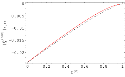
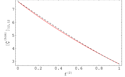
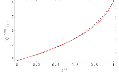
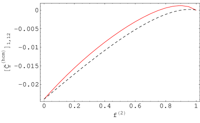
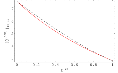
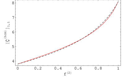
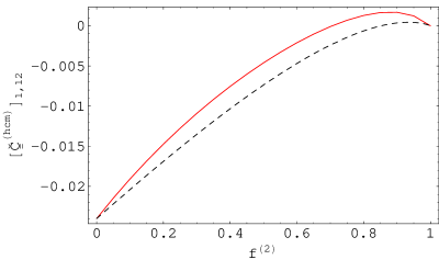
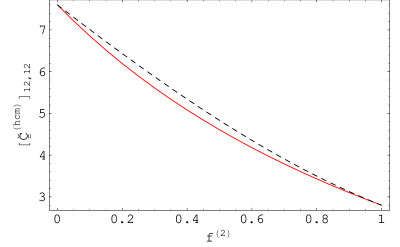
We begin by considering the lowest–order SPFT estimates of the HCM constitutive parameters. In Fig. 1, components of the HCM extended stiffness matrix 𝐂¯¯˘(hcm)superscript˘¯¯𝐂𝑐𝑚\breve{\underline{\underline{\bf C}}}^{(hcm)}, as computed using the lowest–order SPFT and the Mori–Tanaka formalism, are plotted as functions of volume fraction f(2)superscript𝑓2f^{(2)} for the case where the component particles are spherical (i.e., a=b=c𝑎𝑏𝑐a=b=c). Plots of only a representative selection of the components of 𝐂¯¯˘(hcm)superscript˘¯¯𝐂𝑐𝑚\breve{\underline{\underline{\bf C}}}^{(hcm)} are presented in Fig. 1; plots for those components which are not presented in Fig. 1 are qualitatively similar to those that are presented. Only relatively minor differences between the lowest–order SPFT estimates and the Mori–Tanaka estimates are observed, with the differences between the two being greatest for mid–range values of f(2)superscript𝑓2f^{(2)}. Plots for both the SPFT and Mori–Tanaka estimates are necessarily constrained by the limits

limf(2)0𝐂¯¯˘(hcm)=𝐂¯¯˘(1),limf(2)1𝐂¯¯˘(hcm)=𝐂¯¯˘(2).formulae-sequencesubscriptsuperscript𝑓20superscript˘¯¯𝐂𝑐𝑚superscript˘¯¯𝐂1subscriptsuperscript𝑓21superscript˘¯¯𝐂𝑐𝑚superscript˘¯¯𝐂2\lim_{f^{(2)}\to 0}\breve{\underline{\underline{\bf C}}}^{(hcm)}=\breve{\underline{\underline{\bf C}}}^{(1)},\qquad\lim_{f^{(2)}\to 1}\breve{\underline{\underline{\bf C}}}^{(hcm)}=\breve{\underline{\underline{\bf C}}}^{(2)}. (60)

The corresponding graphs for the cases where the components particles are described by the shape parameters {a/c=5,b/c=1.5}formulae-sequence𝑎𝑐5𝑏𝑐1.5\left\{a/c=5,\,b/c=1.5\right\} and {a/c=10,b/c=2}formulae-sequence𝑎𝑐10𝑏𝑐2\left\{a/c=10,\,b/c=2\right\} are provided in Figs. 2 and 3, respectively. A comparison of Figs. 13 reveals that the differences between the lowest–order SPFT and Mori–Tanaka estimates are accentuated as the component particles become more eccentric in shape, especially at mid–range values of f(2)superscript𝑓2f^{(2)} for the piezoelectric parameters and the dielectric parameters.

3.3 Second–order SPFT estimate

Now let us turn to the second–order SPFT estimates of the HCM constitutive parameters. We considered these quantities as functions of k¯L¯𝑘𝐿\bar{k}L, where k¯¯𝑘\bar{k} is an approximate upper bound on the wavenumbers supported by the HCM, as estimated by [20]

k¯=ω2(ρ¯λ¯+2μ¯+ρ¯μ¯),¯𝑘𝜔2¯𝜌¯𝜆2¯𝜇¯𝜌¯𝜇\bar{k}=\frac{\omega}{2}\left(\sqrt{\frac{\bar{\rho}}{\bar{\lambda}+2\bar{\mu}}}+\sqrt{\frac{\bar{\rho}}{\bar{\mu}}}\right), (61)

wherein

λ¯=16=12(|[𝐂¯¯()]12|+|[𝐂¯¯()]13|+|[𝐂¯¯()]23|)μ¯=16=12(|[𝐂¯¯()]44|+|[𝐂¯¯()]55|+|[𝐂¯¯()]66|)ρ¯=12=12ρ()};cases¯𝜆16subscriptsuperscript21subscriptdelimited-[]superscript¯¯𝐂12subscriptdelimited-[]superscript¯¯𝐂13subscriptdelimited-[]superscript¯¯𝐂23¯𝜇16subscriptsuperscript21subscriptdelimited-[]superscript¯¯𝐂44subscriptdelimited-[]superscript¯¯𝐂55subscriptdelimited-[]superscript¯¯𝐂66¯𝜌12subscriptsuperscript21superscript𝜌\left.\begin{array}[]{l}\bar{\lambda}=\displaystyle{\frac{1}{6}\sum^{2}_{\ell=1}\left(\,\left|\left[\,\underline{\underline{\bf C}}^{(\ell)}\,\right]_{12}\right|+\left|\left[\,\underline{\underline{\bf C}}^{(\ell)}\,\right]_{13}\right|+\left|\left[\,\underline{\underline{\bf C}}^{(\ell)}\,\right]_{23}\right|\,\right)\vspace{6pt}}\\ \bar{\mu}=\displaystyle{\frac{1}{6}\sum^{2}_{\ell=1}\left(\,\left|\left[\,\underline{\underline{\bf C}}^{(\ell)}\,\right]_{44}\right|+\left|\left[\,\underline{\underline{\bf C}}^{(\ell)}\,\right]_{55}\right|+\left|\left[\,\underline{\underline{\bf C}}^{(\ell)}\,\right]_{66}\right|\,\right)\vspace{6pt}}\\ \bar{\rho}=\displaystyle{\frac{1}{2}\,\sum^{2}_{\ell=1}\rho^{(\ell)}}\end{array}\right\}; (62)

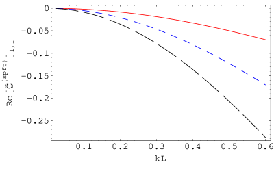
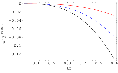
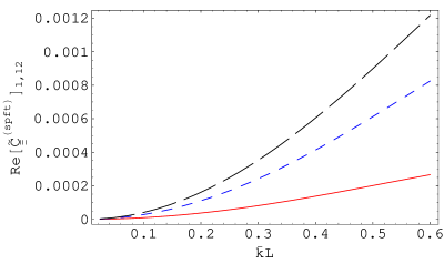
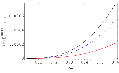
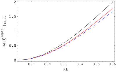
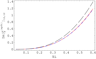
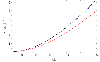
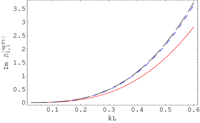
and L𝐿L is the correlation length associated with the the two–point covariance function (18). In Fig. 4, the real and imaginary parts of the components of 𝐂¯~¯(spft)=𝐂¯¯˘(spft)𝐂¯¯˘(ocm)superscript¯¯~𝐂𝑠𝑝𝑓𝑡superscript˘¯¯𝐂𝑠𝑝𝑓𝑡superscript˘¯¯𝐂𝑜𝑐𝑚\underline{\underline{\bf\tilde{C}}}^{(spft)}=\breve{\underline{\underline{\bf C}}}^{(spft)}-\breve{\underline{\underline{\bf C}}}^{(ocm)} are plotted against k¯L¯𝑘𝐿\bar{k}L for f(2)=0.5superscript𝑓20.5f^{(2)}=0.5. The values of the shape parameters {a,b,c}𝑎𝑏𝑐\left\{a,\,b,\,c\right\} correspond to those used in the calculations for Figs. 13. As in §3.2, only a representative selection of the components of 𝐂¯¯~(spft)superscript~¯¯𝐂𝑠𝑝𝑓𝑡\tilde{\underline{\underline{\bf C}}}^{(spft)} are plotted in Fig. 4; the graphs for those components that are not represented in Fig. 4 are qualitatively similar to the graphs which do appear.

The second–order corrections to the lowest–order SPFT estimates are observed in Fig. 4 to grow exponentially in magnitude as the correlation length increases from zero. Furthermore, the magnitudes of both the real and imaginary parts of 𝐂¯¯˘(spft)superscript˘¯¯𝐂𝑠𝑝𝑓𝑡\breve{\underline{\underline{\bf C}}}^{(spft)} generally grow faster with increasingly correlation length when the components particles are more eccentric in shape. At L=0𝐿0L=0, the second–order and lowest–order SPFT estimates coincide. While the second–order corrections are relatively small compared to the lowest–order SPFT estimates, a highly significant feature of the second–order corrections is that these are complex–valued with nonzero imaginary parts, even though 𝐂¯¯˘(a,b)superscript˘¯¯𝐂𝑎𝑏\breve{\underline{\underline{\bf C}}}^{(a,b)} and 𝐂¯¯˘(ocm)superscript˘¯¯𝐂𝑜𝑐𝑚\breve{\underline{\underline{\bf C}}}^{(ocm)} are purely real–valued. We note that for all computations the imaginary part of the extended compliance matrix 𝐌¯¯˘(spft)superscript˘¯¯𝐌𝑠𝑝𝑓𝑡\breve{\underline{\underline{\bf M}}}^{(spft)} was found to be positive definite, which corresponds to positive loss [31]. Thus, the emergence of nonzero imaginary parts of 𝐂¯¯˘(spft)superscript˘¯¯𝐂𝑠𝑝𝑓𝑡\breve{\underline{\underline{\bf C}}}^{(spft)} indicates that the HCM has acquired a dissipative nature, despite the component materials being nondissipative. The dissipation is attributed to scattering losses, since the second–order SPFT takes into account interactions between spatially–distinct scattering particles via the two–point covariance function (18). As the correlation length increases, the number of scattering particles that can mutually interact also increases, thereby increasing the scattering loss per unit volume.

Finally, we turn to the second–order SPFT estimate of the HCM density. The real and imaginary parts of the matrix entry [𝝆¯~¯(spft)]11subscriptdelimited-[]superscriptbold-¯bold-¯bold-~𝝆𝑠𝑝𝑓𝑡11\left[\,\mbox{\boldmath$\underline{\underline{\bf\tilde{\rho}}}$}^{(spft)}\,\right]_{11}, wherein 𝝆¯~¯(spft)=𝝆¯˘¯(spft)𝝆¯˘¯(ocm)superscriptbold-¯bold-¯bold-~𝝆𝑠𝑝𝑓𝑡superscriptbold-¯bold-¯bold-˘𝝆𝑠𝑝𝑓𝑡superscriptbold-¯bold-¯bold-˘𝝆𝑜𝑐𝑚\mbox{\boldmath$\underline{\underline{\bf\tilde{\rho}}}$}^{(spft)}=\mbox{\boldmath$\underline{\underline{\bf\breve{\rho}}}$}^{(spft)}-\mbox{\boldmath$\underline{\underline{\bf\breve{\rho}}}$}^{(ocm)}, are plotted as functions of k¯L¯𝑘𝐿\bar{k}L in Fig. 5. The corresponding graphs for [𝝆¯~¯(spft)]22subscriptdelimited-[]superscriptbold-¯bold-¯bold-~𝝆𝑠𝑝𝑓𝑡22\left[\,\mbox{\boldmath$\underline{\underline{\bf\tilde{\rho}}}$}^{(spft)}\,\right]_{22} and [𝝆¯~¯(spft)]33subscriptdelimited-[]superscriptbold-¯bold-¯bold-~𝝆𝑠𝑝𝑓𝑡33\left[\,\mbox{\boldmath$\underline{\underline{\bf\tilde{\rho}}}$}^{(spft)}\,\right]_{33} are much the same as those for [𝝆¯~¯(spft)]11subscriptdelimited-[]superscriptbold-¯bold-¯bold-~𝝆𝑠𝑝𝑓𝑡11\left[\,\mbox{\boldmath$\underline{\underline{\bf\tilde{\rho}}}$}^{(spft)}\,\right]_{11} but with minor differences in magnitudes. The second–order SPFT estimates of the HCM density exhibit characteristics similar to those of the corresponding HCM stiffness, piezoelectric and dielectric constitutive parameters. That is, limL0ρaa(spft)=ρ(ocm)subscript𝐿0subscriptsuperscript𝜌𝑠𝑝𝑓𝑡𝑎𝑎superscript𝜌𝑜𝑐𝑚\displaystyle{\lim_{L\to 0}\rho^{(spft)}_{aa}=\rho^{(ocm)}} and |ρ~aa(spft)||ρ(ocm)|much-less-thansubscriptsuperscript~𝜌𝑠𝑝𝑓𝑡𝑎𝑎superscript𝜌𝑜𝑐𝑚\Big{|}\tilde{\rho}^{(spft)}_{aa}\Big{|}\ll\Big{|}\rho^{(ocm)}\Big{|} for a=1,2𝑎12a=1,2 and 333. Also, the differences between 𝝆¯˘¯(spft)superscriptbold-¯bold-¯bold-˘𝝆𝑠𝑝𝑓𝑡\mbox{\boldmath$\underline{\underline{\bf\breve{\rho}}}$}^{(spft)} and 𝝆¯˘¯(ocm)superscriptbold-¯bold-¯bold-˘𝝆𝑜𝑐𝑚\mbox{\boldmath$\underline{\underline{\bf\breve{\rho}}}$}^{(ocm)} increase exponentially as the correlation length increases, and this effect is most accentuated when the component particles are most eccentric in shape.

We remark that a complex–valued, anisotropic density also crops up in the second–order elastodynamic SPFT for orthotropic HCMs [20], as well as in other homogenization scenarios [33, 34].

4 Closing remarks

The linear SPFT has been fully developed for the case of orthorhombic mm2𝑚𝑚2mm2 piezoelectric HCMs, based on component materials distributed as oriented ellipsoidal particles. The multifunctionality of such HCMs is central to the notion of metamaterials [5]. The second–order estimates of the HCM constitutive parameters are expressed in terms of numerically–tractable two–dimensional integrals, for a specific choice of two–point covariance function. This theoretical result further extends the application of the SPFT in the homogenization of complex composites, effectively bridging the elastodynamic SPFT for orthotropic HCMs [19, 20] and the electromagnetic SPFT for anisotropic dielectric HCMs [35, 36]. Furthermore, the path has now been cleared towards the development of the SPFT for piezoelectric/piezomagnetic HCMs [37], with bianisotropic electromagnetic properties [17]. Let us remark that the mathematical description of piezoelectric HCMs presented herein also extends to electrokinetic processes [38].

From our theoretical considerations and representative numerical studies, the following conclusions were drawn:

  • The lowest–order SPFT estimate of the stiffness, piezoelectric and dielectric properties of the HCM are qualitatively similar to those estimates provided by the Mori–Tanaka formalism.

  • Differences between the estimates of the lowest–order SPFT and the Mori–Tanaka formalism are greatest at mid–range values of the volume fraction, and accentuated when the component particles are eccentric in shape.

  • The second–order SPFT provides a correction to the lowest–order estimate of the HCM constitutive properties. The magnitude of this correction is generally larger when the component particles are more eccentric in shape, and vanishes as the correlation length tends to zero.

  • While the correction provided by the second–order SPFT is relatively small in magnitude, it is highly significant as it indicates dissipation due to scattering loss.

Appendix A

The extended symbol A˘aMPqsubscript˘𝐴𝑎𝑀𝑃𝑞\breve{A}_{aMPq} (a,q{1,2,3}𝑎𝑞123a,q\in\left\{1,2,3\right\}, M,P{1,2,3,4}𝑀𝑃1234M,P\in\left\{1,2,3,4\right\}) may be conveniently represented by the 12×12121212\times 12 matrix with entries [𝐀¯¯˘]γκsubscriptdelimited-[]˘¯¯𝐀𝛾𝜅\left[\breve{\underline{\underline{\bf A}}}\right]_{\gamma\kappa} (γ,κ[1,12]𝛾𝜅112\gamma,\kappa\in\left[1,12\right]), upon replacing the index pair aM𝑎𝑀aM with γ𝛾\gamma and the index pair Pq𝑃𝑞Pq with κ𝜅\kappa. For the most general 12×\times12 matrix encountered in this paper, which has the form

𝐀¯¯˘=(A1,1A1,2A1,300000000A1,12A2,1A2,2A2,300000000A2,12A3,1A3,2A3,300000000A3,12000A4,400A4,4000A4,1100000A5,500A5,50A5,100000000A6,600A6,6000000A4,400A4,4000A4,1100000A5,500A5,50A5,100000000A6,600A6,60000000A10,500A10,50A10,1000000A11,400A11,4000A11,110A12,1A12,2A12,300000000A12,12),˘¯¯𝐀subscript𝐴11subscript𝐴12subscript𝐴1300000000subscript𝐴112subscript𝐴21subscript𝐴22subscript𝐴2300000000subscript𝐴212subscript𝐴31subscript𝐴32subscript𝐴3300000000subscript𝐴312000subscript𝐴4400subscript𝐴44000subscript𝐴41100000subscript𝐴5500subscript𝐴550subscript𝐴5100000000subscript𝐴6600subscript𝐴66000000subscript𝐴4400subscript𝐴44000subscript𝐴41100000subscript𝐴5500subscript𝐴550subscript𝐴5100000000subscript𝐴6600subscript𝐴660000000subscript𝐴10500subscript𝐴1050subscript𝐴101000000subscript𝐴11400subscript𝐴114000subscript𝐴11110subscript𝐴121subscript𝐴122subscript𝐴12300000000subscript𝐴1212\breve{\underline{\underline{\bf A}}}=\left(\begin{array}[]{cccccccccccc}A_{1,1}&A_{1,2}&A_{1,3}&0&0&0&0&0&0&0&0&A_{1,12}\\ A_{2,1}&A_{2,2}&A_{2,3}&0&0&0&0&0&0&0&0&A_{2,12}\\ A_{3,1}&A_{3,2}&A_{3,3}&0&0&0&0&0&0&0&0&A_{3,12}\\ 0&0&0&A_{4,4}&0&0&A_{4,4}&0&0&0&A_{4,11}&0\\ 0&0&0&0&A_{5,5}&0&0&A_{5,5}&0&A_{5,10}&0&0\\ 0&0&0&0&0&A_{6,6}&0&0&A_{6,6}&0&0&0\\ 0&0&0&A_{4,4}&0&0&A_{4,4}&0&0&0&A_{4,11}&0\\ 0&0&0&0&A_{5,5}&0&0&A_{5,5}&0&A_{5,10}&0&0\\ 0&0&0&0&0&A_{6,6}&0&0&A_{6,6}&0&0&0\\ 0&0&0&0&A_{10,5}&0&0&A_{10,5}&0&A_{10,10}&0&0\\ 0&0&0&A_{11,4}&0&0&A_{11,4}&0&0&0&A_{11,11}&0\\ A_{12,1}&A_{12,2}&A_{12,3}&0&0&0&0&0&0&0&0&A_{12,12}\\ \end{array}\right), (63)

the correspondence between the extended symbol indexes and the matrix indexes is provided in Table 2. The scheme presented in Table 2 also relates the extended symbol t˘aMsubscript˘𝑡𝑎𝑀\breve{t}_{aM} to the corresponding column 12–vector entries [𝐭˘]γsubscriptdelimited-[]˘𝐭𝛾\left[\,\breve{{\bf t}}\,\right]_{\gamma}.

aM𝑎𝑀aM or Pq𝑃𝑞Pq γ𝛾\gamma or κ𝜅\kappa aM𝑎𝑀aM or Pq𝑃𝑞Pq γ𝛾\gamma or κ𝜅\kappa aM𝑎𝑀aM or Pq𝑃𝑞Pq γ𝛾\gamma or κ𝜅\kappa aM𝑎𝑀aM or Pq𝑃𝑞Pq γ𝛾\gamma or κ𝜅\kappa
111111 111 232323 or 323232 444 232323 or 323232 777 141414 or 414141 101010
222222 222 131313 or 313131 555 131313 or 313131 888 242424 or 424242 111111
333333 333 121212 or 212121 666 121212 or 212121 999 343434 or 434343 121212
Table 2: Conversion between extended symbol and matrix notation.

We introduce the matrix 𝐀¯¯˘superscript˘¯¯𝐀\breve{\underline{\underline{\bf A}}}^{\dagger} which plays a role similar to the matrix inverse insofar as

𝐀¯¯˘𝐀¯¯˘=𝐀¯¯˘𝐀¯¯˘=𝝉¯¯.superscript˘¯¯𝐀˘¯¯𝐀˘¯¯𝐀superscript˘¯¯𝐀bold-¯bold-¯𝝉\breve{\underline{\underline{\bf A}}}^{\dagger}\cdot\breve{\underline{\underline{\bf A}}}=\breve{\underline{\underline{\bf A}}}\cdot\breve{\underline{\underline{\bf A}}}^{\dagger}=\mbox{\boldmath$\underline{\underline{\bf\tau}}$}. (64)

Herein,

𝝉¯¯=(𝐈¯¯𝟎¯¯ 3×3𝟎¯¯ 3×3𝟎¯¯ 3×3𝟎¯¯ 3×312𝐈¯¯12𝐈¯¯𝟎¯¯ 3×3𝟎¯¯ 3×312𝐈¯¯12𝐈¯¯𝟎¯¯ 3×3𝟎¯¯ 3×3𝟎¯¯ 3×3𝟎¯¯ 3×3𝐈¯¯)bold-¯bold-¯𝝉¯¯𝐈subscript¯¯033subscript¯¯033subscript¯¯033subscript¯¯03312¯¯𝐈12¯¯𝐈subscript¯¯033subscript¯¯03312¯¯𝐈12¯¯𝐈subscript¯¯033subscript¯¯033subscript¯¯033subscript¯¯033¯¯𝐈\mbox{\boldmath$\underline{\underline{\bf\tau}}$}=\left(\begin{array}[]{llll}\underline{\underline{\bf I}}&\underline{\underline{\bf 0}}_{\,3\times 3}&\underline{\underline{\bf 0}}_{\,3\times 3}&\underline{\underline{\bf 0}}_{\,3\times 3}\vspace{4pt}\\ \underline{\underline{\bf 0}}_{\,3\times 3}&\frac{1}{2}\underline{\underline{\bf I}}&\frac{1}{2}\underline{\underline{\bf I}}&\underline{\underline{\bf 0}}_{\,3\times 3}\vspace{4pt}\\ \underline{\underline{\bf 0}}_{\,3\times 3}&\frac{1}{2}\underline{\underline{\bf I}}&\frac{1}{2}\underline{\underline{\bf I}}&\underline{\underline{\bf 0}}_{\,3\times 3}\vspace{4pt}\\ \underline{\underline{\bf 0}}_{\,3\times 3}&\underline{\underline{\bf 0}}_{\,3\times 3}&\underline{\underline{\bf 0}}_{\,3\times 3}&\underline{\underline{\bf I}}\end{array}\right) (65)

is the 12×\times12 matrix representation of the extended identity symbol, with 𝐈¯¯¯¯𝐈\underline{\underline{\bf I}} being the 3×\times3 identity matrix, and we have

𝐀¯¯˘𝝉¯¯=𝝉¯¯𝐀¯¯˘=𝐀¯¯˘.˘¯¯𝐀bold-¯bold-¯𝝉bold-¯bold-¯𝝉˘¯¯𝐀˘¯¯𝐀\breve{\underline{\underline{\bf A}}}\cdot\mbox{\boldmath$\underline{\underline{\bf\tau}}$}=\mbox{\boldmath$\underline{\underline{\bf\tau}}$}\cdot\breve{\underline{\underline{\bf A}}}=\breve{\underline{\underline{\bf A}}}. (66)

The matrix 𝐀¯¯˘superscript˘¯¯𝐀\breve{\underline{\underline{\bf A}}}^{\dagger} has the form

𝐀¯¯˘=(1,11,21,3000000001,122,12,22,3000000002,123,13,23,3000000003,120004,42004,420004,11000005,52005,5205,1000000006,62006,620000004,42004,420004,11000005,52005,5205,1000000006,62006,62000000010,50010,5010,100000011,40011,400011,11012,112,212,30000000012,12),superscript˘¯¯𝐀subscript11subscript12subscript1300000000subscript112subscript21subscript22subscript2300000000subscript212subscript31subscript32subscript3300000000subscript312000subscript44200subscript442000subscript41100000subscript55200subscript5520subscript5100000000subscript66200subscript662000000subscript44200subscript442000subscript41100000subscript55200subscript5520subscript5100000000subscript66200subscript6620000000subscript10500subscript1050subscript101000000subscript11400subscript114000subscript11110subscript121subscript122subscript12300000000subscript1212\breve{\underline{\underline{\bf A}}}^{\dagger}=\left(\begin{array}[]{cccccccccccc}\dagger_{1,1}&\dagger_{1,2}&\dagger_{1,3}&0&0&0&0&0&0&0&0&\dagger_{1,12}\\ \dagger_{2,1}&\dagger_{2,2}&\dagger_{2,3}&0&0&0&0&0&0&0&0&\dagger_{2,12}\\ \dagger_{3,1}&\dagger_{3,2}&\dagger_{3,3}&0&0&0&0&0&0&0&0&\dagger_{3,12}\\ 0&0&0&\frac{\dagger_{4,4}}{2}&0&0&\frac{\dagger_{4,4}}{2}&0&0&0&\dagger_{4,11}&0\\ 0&0&0&0&\frac{\dagger_{5,5}}{2}&0&0&\frac{\dagger_{5,5}}{2}&0&\dagger_{5,10}&0&0\\ 0&0&0&0&0&\frac{\dagger_{6,6}}{2}&0&0&\frac{\dagger_{6,6}}{2}&0&0&0\\ 0&0&0&\frac{\dagger_{4,4}}{2}&0&0&\frac{\dagger_{4,4}}{2}&0&0&0&\dagger_{4,11}&0\\ 0&0&0&0&\frac{\dagger_{5,5}}{2}&0&0&\frac{\dagger_{5,5}}{2}&0&\dagger_{5,10}&0&0\\ 0&0&0&0&0&\frac{\dagger_{6,6}}{2}&0&0&\frac{\dagger_{6,6}}{2}&0&0&0\\ 0&0&0&0&\dagger_{10,5}&0&0&\dagger_{10,5}&0&\dagger_{10,10}&0&0\\ 0&0&0&\dagger_{11,4}&0&0&\dagger_{11,4}&0&0&0&\dagger_{11,11}&0\\ \dagger_{12,1}&\dagger_{12,2}&\dagger_{12,3}&0&0&0&0&0&0&0&0&\dagger_{12,12}\\ \end{array}\right), (67)

with entries

1,1subscript11\displaystyle\dagger_{1,1} =\displaystyle= (A12,3A2,2A3,12+A12,2A2,3A3,12+A12,3A2,12A3,2A12,12A2,3A3,2\displaystyle(-A_{12,3}A_{2,2}A_{3,12}+A_{12,2}A_{2,3}A_{3,12}+A_{12,3}A_{2,12}A_{3,2}-A_{12,12}A_{2,3}A_{3,2}- (68)
A12,2A2,12A3,3+A12,12A2,2A3,3)/Λ,\displaystyle A_{12,2}A_{2,12}A_{3,3}+A_{12,12}A_{2,2}A_{3,3})/\Lambda,
1,2subscript12\displaystyle\dagger_{1,2} =\displaystyle= (A1,2A12,3A3,12A12,2A1,3A3,12A1,12A12,3A3,2+A12,12A1,3A3,2\displaystyle(A_{1,2}A_{12,3}A_{3,12}-A_{12,2}A_{1,3}A_{3,12}-A_{1,12}A_{12,3}A_{3,2}+A_{12,12}A_{1,3}A_{3,2}- (69)
A1,2A12,12A3,3+A1,12A12,2A3,3)/Λ,\displaystyle A_{1,2}A_{12,12}A_{3,3}+A_{1,12}A_{12,2}A_{3,3})/\Lambda,
1,3subscript13\displaystyle\dagger_{1,3} =\displaystyle= (A1,2A12,3A2,12+A12,2A1,3A2,12+A1,12A12,3A2,2A12,12A1,3A2,2+\displaystyle(-A_{1,2}A_{12,3}A_{2,12}+A_{12,2}A_{1,3}A_{2,12}+A_{1,12}A_{12,3}A_{2,2}-A_{12,12}A_{1,3}A_{2,2}+ (70)
A1,2A12,12A2,3A1,12A12,2A2,3)/Λ,\displaystyle A_{1,2}A_{12,12}A_{2,3}-A_{1,12}A_{12,2}A_{2,3})/\Lambda,
2,1subscript21\displaystyle\dagger_{2,1} =\displaystyle= (A12,3A2,12A3,1+A12,12A2,3A3,1+A12,3A2,1A3,12A12,1A2,3A3,12\displaystyle(-A_{12,3}A_{2,12}A_{3,1}+A_{12,12}A_{2,3}A_{3,1}+A_{12,3}A_{2,1}A_{3,12}-A_{12,1}A_{2,3}A_{3,12}- (71)
A12,12A2,1A3,3+A12,1A2,12A3,3)/Λ,\displaystyle A_{12,12}A_{2,1}A_{3,3}+A_{12,1}A_{2,12}A_{3,3})/\Lambda,
2,2subscript22\displaystyle\dagger_{2,2} =\displaystyle= (A1,12A12,3A3,1A12,12A1,3A3,1A1,1A12,3A3,12+A12,1A1,3A3,12\displaystyle(A_{1,12}A_{12,3}A_{3,1}-A_{12,12}A_{1,3}A_{3,1}-A_{1,1}A_{12,3}A_{3,12}+A_{12,1}A_{1,3}A_{3,12}- (72)
A1,12A12,1A3,3+A1,1A12,12A3,3)/Λ,\displaystyle A_{1,12}A_{12,1}A_{3,3}+A_{1,1}A_{12,12}A_{3,3})/\Lambda,
2,3subscript23\displaystyle\dagger_{2,3} =\displaystyle= (A1,12A12,3A2,1+A12,12A1,3A2,1+A1,1A12,3A2,12A12,1A1,3A2,12+\displaystyle(-A_{1,12}A_{12,3}A_{2,1}+A_{12,12}A_{1,3}A_{2,1}+A_{1,1}A_{12,3}A_{2,12}-A_{12,1}A_{1,3}A_{2,12}+ (73)
A1,12A12,1A2,3A1,1A12,12A2,3)/Λ,\displaystyle A_{1,12}A_{12,1}A_{2,3}-A_{1,1}A_{12,12}A_{2,3})/\Lambda,
3,1subscript31\displaystyle\dagger_{3,1} =\displaystyle= (A12,2A2,12A3,1A12,12A2,2A3,1A12,2A2,1A3,12+A12,1A2,2A3,12+\displaystyle(A_{12,2}A_{2,12}A_{3,1}-A_{12,12}A_{2,2}A_{3,1}-A_{12,2}A_{2,1}A_{3,12}+A_{12,1}A_{2,2}A_{3,12}+ (74)
A12,12A2,1A3,2A12,1A2,12A3,2)/Λ,\displaystyle A_{12,12}A_{2,1}A_{3,2}-A_{12,1}A_{2,12}A_{3,2})/\Lambda,
3,2subscript32\displaystyle\dagger_{3,2} =\displaystyle= (A1,2A12,12A3,1A1,12A12,2A3,1A1,2A12,1A3,12+A1,1A12,2A3,12+\displaystyle(A_{1,2}A_{12,12}A_{3,1}-A_{1,12}A_{12,2}A_{3,1}-A_{1,2}A_{12,1}A_{3,12}+A_{1,1}A_{12,2}A_{3,12}+ (75)
A1,12A12,1A3,2A1,1A12,12A3,2)/Λ,\displaystyle A_{1,12}A_{12,1}A_{3,2}-A_{1,1}A_{12,12}A_{3,2})/\Lambda,
3,3subscript33\displaystyle\dagger_{3,3} =\displaystyle= (A1,2A12,12A2,1+A1,12A12,2A2,1+A1,2A12,1A2,12A1,1A12,2A2,12\displaystyle(-A_{1,2}A_{12,12}A_{2,1}+A_{1,12}A_{12,2}A_{2,1}+A_{1,2}A_{12,1}A_{2,12}-A_{1,1}A_{12,2}A_{2,12}- (76)
A1,12A12,1A2,2+A1,1A12,12A2,2)/Λ,\displaystyle A_{1,12}A_{12,1}A_{2,2}+A_{1,1}A_{12,12}A_{2,2})/\Lambda,
4,4subscript44\displaystyle\dagger_{4,4} =\displaystyle= A11,112(A11,11A4,4A4,11A11,4),subscript𝐴11112subscript𝐴1111subscript𝐴44subscript𝐴411subscript𝐴114\displaystyle\frac{A_{11,11}}{2(A_{11,11}A_{4,4}-A_{4,11}A_{11,4})}, (77)
5,5subscript55\displaystyle\dagger_{5,5} =\displaystyle= A10,102(A10,10A5,5A5,10A10,5),subscript𝐴10102subscript𝐴1010subscript𝐴55subscript𝐴510subscript𝐴105\displaystyle\frac{A_{10,10}}{2(A_{10,10}A_{5,5}-A_{5,10}A_{10,5})}, (78)
6,6subscript66\displaystyle\dagger_{6,6} =\displaystyle= 12A6,6,12subscript𝐴66\displaystyle\frac{1}{2A_{6,6}}, (79)
10,10subscript1010\displaystyle\dagger_{10,10} =\displaystyle= A5,5(A10,10A5,5A10,5A5,10),subscript𝐴55subscript𝐴1010subscript𝐴55subscript𝐴105subscript𝐴510\displaystyle\frac{A_{5,5}}{(A_{10,10}A_{5,5}-A_{10,5}A_{5,10})}, (80)
11,11subscript1111\displaystyle\dagger_{11,11} =\displaystyle= A4,4(A11,11A4,4A11,4A4,11),subscript𝐴44subscript𝐴1111subscript𝐴44subscript𝐴114subscript𝐴411\displaystyle\frac{A_{4,4}}{(A_{11,11}A_{4,4}-A_{11,4}A_{4,11})}, (81)
12,12subscript1212\displaystyle\dagger_{12,12} =\displaystyle= (A1,3A2,2A3,1+A1,2A2,3A3,1+A1,3A2,1A3,2A1,1A2,3A3,2\displaystyle(-A_{1,3}A_{2,2}A_{3,1}+A_{1,2}A_{2,3}A_{3,1}+A_{1,3}A_{2,1}A_{3,2}-A_{1,1}A_{2,3}A_{3,2}- (82)
A1,2A2,1A3,3+A1,1A2,2A3,3)/Λ,\displaystyle A_{1,2}A_{2,1}A_{3,3}+A_{1,1}A_{2,2}A_{3,3})/\Lambda,
1,12subscript112\displaystyle\dagger_{1,12} =\displaystyle= (A1,3A2,2A3,12A1,2A2,3A3,12A1,3A2,12A3,2+A1,12A2,3A3,2+\displaystyle(A_{1,3}A_{2,2}A_{3,12}-A_{1,2}A_{2,3}A_{3,12}-A_{1,3}A_{2,12}A_{3,2}+A_{1,12}A_{2,3}A_{3,2}+ (83)
A1,2A2,12A3,3A1,12A2,2A3,3)/Λ,\displaystyle A_{1,2}A_{2,12}A_{3,3}-A_{1,12}A_{2,2}A_{3,3})/\Lambda,
2,12subscript212\displaystyle\dagger_{2,12} =\displaystyle= (A1,3A2,12A3,1A1,12A2,3A3,1A1,3A2,1A3,12+A1,1A2,3A3,12+\displaystyle(A_{1,3}A_{2,12}A_{3,1}-A_{1,12}A_{2,3}A_{3,1}-A_{1,3}A_{2,1}A_{3,12}+A_{1,1}A_{2,3}A_{3,12}+ (84)
A1,12A2,1A3,3A1,1A2,12A3,3)/Λ,\displaystyle A_{1,12}A_{2,1}A_{3,3}-A_{1,1}A_{2,12}A_{3,3})/\Lambda,
3,12subscript312\displaystyle\dagger_{3,12} =\displaystyle= (A1,2A2,12A3,1+A1,12A2,2A3,1+A1,2A2,1A3,12A1,1A2,2A3,12\displaystyle(-A_{1,2}A_{2,12}A_{3,1}+A_{1,12}A_{2,2}A_{3,1}+A_{1,2}A_{2,1}A_{3,12}-A_{1,1}A_{2,2}A_{3,12}- (85)
A1,12A2,1A3,2+A1,1A2,12A3,2)/Λ,\displaystyle A_{1,12}A_{2,1}A_{3,2}+A_{1,1}A_{2,12}A_{3,2})/\Lambda,
4,11subscript411\displaystyle\dagger_{4,11} =\displaystyle= A4,112(A11,4A4,11A11,11A4,4),subscript𝐴4112subscript𝐴114subscript𝐴411subscript𝐴1111subscript𝐴44\displaystyle\frac{A_{4,11}}{2(A_{11,4}A_{4,11}-A_{11,11}A_{4,4})}, (86)
5,10subscript510\displaystyle\dagger_{5,10} =\displaystyle= A5,102(A5,10A10,5A10,10A5,5),subscript𝐴5102subscript𝐴510subscript𝐴105subscript𝐴1010subscript𝐴55\displaystyle\frac{A_{5,10}}{2(A_{5,10}A_{10,5}-A_{10,10}A_{5,5})}, (87)
12,1subscript121\displaystyle\dagger_{12,1} =\displaystyle= (A12,3A2,2A3,1A12,2A2,3A3,1A12,3A2,1A3,2+A12,1A2,3A3,2+\displaystyle(A_{12,3}A_{2,2}A_{3,1}-A_{12,2}A_{2,3}A_{3,1}-A_{12,3}A_{2,1}A_{3,2}+A_{12,1}A_{2,3}A_{3,2}+ (88)
A12,2A2,1A3,3A12,1A2,2A3,3)/Λ,\displaystyle A_{12,2}A_{2,1}A_{3,3}-A_{12,1}A_{2,2}A_{3,3})/\Lambda,
12,2subscript122\displaystyle\dagger_{12,2} =\displaystyle= (A1,2A12,3A3,1+A12,2A1,3A3,1+A1,1A12,3A3,2A12,1A1,3A3,2+\displaystyle(-A_{1,2}A_{12,3}A_{3,1}+A_{12,2}A_{1,3}A_{3,1}+A_{1,1}A_{12,3}A_{3,2}-A_{12,1}A_{1,3}A_{3,2}+ (89)
A1,2A12,1A3,3A1,1A12,2A3,3)/Λ,\displaystyle A_{1,2}A_{12,1}A_{3,3}-A_{1,1}A_{12,2}A_{3,3})/\Lambda,
12,3subscript123\displaystyle\dagger_{12,3} =\displaystyle= (A1,2A12,3A2,1A12,2A1,3A2,1A1,1A12,3A2,2+A12,1A1,3A2,2\displaystyle(A_{1,2}A_{12,3}A_{2,1}-A_{12,2}A_{1,3}A_{2,1}-A_{1,1}A_{12,3}A_{2,2}+A_{12,1}A_{1,3}A_{2,2}- (90)
A1,2A12,1A2,3+A1,1A12,2A2,3)/Λ,\displaystyle A_{1,2}A_{12,1}A_{2,3}+A_{1,1}A_{12,2}A_{2,3})/\Lambda,
11,4subscript114\displaystyle\dagger_{11,4} =\displaystyle= A11,42(A11,4A4,11A11,11A4,4),subscript𝐴1142subscript𝐴114subscript𝐴411subscript𝐴1111subscript𝐴44\displaystyle\frac{A_{11,4}}{2(A_{11,4}A_{4,11}-A_{11,11}A_{4,4})}, (91)
10,5subscript105\displaystyle\dagger_{10,5} =\displaystyle= A10,52(A10,5A5,10A10,10A5,5),subscript𝐴1052subscript𝐴105subscript𝐴510subscript𝐴1010subscript𝐴55\displaystyle\frac{A_{10,5}}{2(A_{10,5}A_{5,10}-A_{10,10}A_{5,5})}, (92)

where the scalar

ΛΛ\displaystyle\Lambda =\displaystyle= A1,12A12,3A2,2A3,1A12,12A1,3A2,2A3,1A1,1A12,3A2,2A3,12+A12,1A1,3A2,2A3,12subscript𝐴112subscript𝐴123subscript𝐴22subscript𝐴31subscript𝐴1212subscript𝐴13subscript𝐴22subscript𝐴31subscript𝐴11subscript𝐴123subscript𝐴22subscript𝐴312limit-fromsubscript𝐴121subscript𝐴13subscript𝐴22subscript𝐴312\displaystyle A_{1,12}A_{12,3}A_{2,2}A_{3,1}-A_{12,12}A_{1,3}A_{2,2}A_{3,1}-A_{1,1}A_{12,3}A_{2,2}A_{3,12}+A_{12,1}A_{1,3}A_{2,2}A_{3,12}- (94)
A1,12A12,3A2,1A3,2+A12,12A1,3A2,1A3,2+A1,1A12,3A2,12A3,2A12,1A1,3A2,12A3,2+subscript𝐴112subscript𝐴123subscript𝐴21subscript𝐴32subscript𝐴1212subscript𝐴13subscript𝐴21subscript𝐴32subscript𝐴11subscript𝐴123subscript𝐴212subscript𝐴32limit-fromsubscript𝐴121subscript𝐴13subscript𝐴212subscript𝐴32\displaystyle A_{1,12}A_{12,3}A_{2,1}A_{3,2}+A_{12,12}A_{1,3}A_{2,1}A_{3,2}+A_{1,1}A_{12,3}A_{2,12}A_{3,2}-A_{12,1}A_{1,3}A_{2,12}A_{3,2}+
A1,12A12,1A2,3A3,2A1,1A12,12A2,3A3,2A1,12A12,1A2,2A3,3+A1,1A12,12A2,2A3,3+subscript𝐴112subscript𝐴121subscript𝐴23subscript𝐴32subscript𝐴11subscript𝐴1212subscript𝐴23subscript𝐴32subscript𝐴112subscript𝐴121subscript𝐴22subscript𝐴33limit-fromsubscript𝐴11subscript𝐴1212subscript𝐴22subscript𝐴33\displaystyle A_{1,12}A_{12,1}A_{2,3}A_{3,2}-A_{1,1}A_{12,12}A_{2,3}A_{3,2}-A_{1,12}A_{12,1}A_{2,2}A_{3,3}+A_{1,1}A_{12,12}A_{2,2}A_{3,3}+
A12,2(A1,3A2,12A3,1A1,12A2,3A3,1A1,3A2,1A3,12+A1,1A2,3A3,12+\displaystyle A_{12,2}(A_{1,3}A_{2,12}A_{3,1}-A_{1,12}A_{2,3}A_{3,1}-A_{1,3}A_{2,1}A_{3,12}+A_{1,1}A_{2,3}A_{3,12}+
A1,12A2,1A3,3A1,1A2,12A3,3)+A1,2(A12,3A2,12A3,1+A12,12A2,3A3,1+\displaystyle A_{1,12}A_{2,1}A_{3,3}-A_{1,1}A_{2,12}A_{3,3})+A_{1,2}(-A_{12,3}A_{2,12}A_{3,1}+A_{12,12}A_{2,3}A_{3,1}+
A12,3A2,1A3,12A12,1A2,3A3,12A12,12A2,1A3,3+A12,1A2,12A3,3).\displaystyle A_{12,3}A_{2,1}A_{3,12}-A_{12,1}A_{2,3}A_{3,12}-A_{12,12}A_{2,1}A_{3,3}+A_{12,1}A_{2,12}A_{3,3}).

Appendix B

The extended Eshelby symbol appropriate to orthorhombic mm2𝑚𝑚2mm2 piezoelectric materials, distributed as ellipsoidal particles with shape parameters {a,b,c}𝑎𝑏𝑐\left\{a,b,c\right\}, is given by [10, 32]

SMnAb(esh)={18πCsJAb(1)1+1𝑑ζ302π𝑑ω[FmJsn(ϑ¯)+FnJsm(ϑ¯)],M=m=1, 2, 314πCsJAb(1)1+1𝑑ζ302π𝑑ωF4Jsn(ϑ¯),M=4,subscriptsuperscript𝑆𝑒𝑠𝑀𝑛𝐴𝑏cases18𝜋subscriptsuperscript𝐶1𝑠𝐽𝐴𝑏superscriptsubscript11differential-dsubscript𝜁3superscriptsubscript02𝜋differential-d𝜔delimited-[]subscript𝐹𝑚𝐽𝑠𝑛¯italic-ϑsubscript𝐹𝑛𝐽𝑠𝑚¯italic-ϑmissing-subexpressionformulae-sequence𝑀𝑚123missing-subexpressionmissing-subexpressionmissing-subexpression14𝜋subscriptsuperscript𝐶1𝑠𝐽𝐴𝑏superscriptsubscript11differential-dsubscript𝜁3superscriptsubscript02𝜋differential-d𝜔subscript𝐹4𝐽𝑠𝑛¯italic-ϑmissing-subexpression𝑀4S^{(esh)}_{MnAb}=\left\{\begin{array}[]{lcr}\displaystyle{\frac{1}{8\pi}C^{(1)}_{sJAb}\int_{-1}^{+1}d\zeta_{3}\int_{0}^{2\pi}d\omega\;\left[\,F_{mJsn}(\overline{\vartheta})+F_{nJsm}(\overline{\vartheta})\,\right]},&&M=m=1,\,2,\,3\\ &\\ \displaystyle{\frac{1}{4\pi}C^{(1)}_{sJAb}\int_{-1}^{+1}d\zeta_{3}\int_{0}^{2\pi}d\omega\;\,F_{4Jsn}(\overline{\vartheta})\,},&&M=4\end{array}\right., (95)

wherein

FMJsn(ϑ¯)=ϑ¯sϑ¯nKMJ1,KJR=ϑ¯sCsJRn(1)ϑ¯nϑ¯1=ζ1a,ϑ¯2=ζ2b,ϑ¯3=ζ3cζ1=(1ζ32)1/2cos(ω),ζ2=(1ζ32)1/2sin(ω),ζ3=ζ3}.casesformulae-sequencesubscript𝐹𝑀𝐽𝑠𝑛¯italic-ϑsubscript¯italic-ϑ𝑠subscript¯italic-ϑ𝑛superscriptsubscript𝐾𝑀𝐽1subscript𝐾𝐽𝑅subscript¯italic-ϑ𝑠subscriptsuperscript𝐶1𝑠𝐽𝑅𝑛subscript¯italic-ϑ𝑛formulae-sequencesubscript¯italic-ϑ1subscript𝜁1𝑎formulae-sequencesubscript¯italic-ϑ2subscript𝜁2𝑏subscript¯italic-ϑ3subscript𝜁3𝑐formulae-sequencesubscript𝜁1superscript1superscriptsubscript𝜁3212𝜔formulae-sequencesubscript𝜁2superscript1superscriptsubscript𝜁3212𝜔subscript𝜁3subscript𝜁3\left.\begin{array}[]{l}\displaystyle{F_{MJsn}(\overline{\vartheta})=\overline{\vartheta}_{s}\overline{\vartheta}_{n}K_{MJ}^{-1},\qquad K_{JR}=\overline{\vartheta}_{s}C^{(1)}_{sJRn}\overline{\vartheta}_{n}\vspace{4pt}}\\ \displaystyle{\overline{\vartheta}_{1}=\frac{\zeta_{1}}{a},\qquad\overline{\vartheta}_{2}=\frac{\zeta_{2}}{b},\qquad\overline{\vartheta}_{3}=\frac{\zeta_{3}}{c}\vspace{4pt}}\\ \displaystyle{\zeta_{1}=(1-\zeta_{3}^{2})^{1/2}\cos(\omega),\qquad\zeta_{2}=(1-\zeta_{3}^{2})^{1/2}\sin(\omega),\qquad\zeta_{3}=\zeta_{3}}\end{array}\right\}. (96)

The integrals in eqs. (95) can be evaluated using standard numerical methods [30].

The conversion from the extended Eshelby symbol SMnAb(esh)subscriptsuperscript𝑆𝑒𝑠𝑀𝑛𝐴𝑏S^{(esh)}_{MnAb} to the extended Eshelby 12×\times12 matrix, namely 𝐒¯¯(Esh)superscript¯¯𝐒𝐸𝑠\underline{\underline{\bf S}}^{(Esh)}, follows the scheme described in Appendix A.

Acknowledgement: AJD is supported by an Engineering and Physical Sciences Research Council (UK) studentship.

References

  • [1] Ting R Y 1986 Evaluation of new piezoelectric composite materials for hydrophone applications Ferroelectrics 67 143–157
  • [2] Zhang R, Jiang B and Cao W 2001 Elastic, piezoelectric, and dielectric properties of multidomain 0.67Pb(Mg1/3Nb2/3)O30.33PbTiO30.67PbsubscriptMg13subscriptNb23subscriptO30.33subscriptPbTiO30.67\mbox{Pb}(\mbox{Mg}_{1/3}\mbox{Nb}_{2/3})\mbox{O}_{3}-0.33\mbox{PbTiO}_{3} single crystals J. Appl. Phys. 90 3471–3475
  • [3] Damjanovic D 1998 Ferroelectric, dielectric and piezoelectric properties of ferroelectric thin films and ceramics Rep. Prog. Phys. 61 1267 -1324
  • [4] Swallow L M, Luo J K, Siores E, Patel I and Dodds D 2008 A piezoelectric fibre composite based energy harvesting device for potential wearable applications Smart Mater. Struct. 17 025017
  • [5] Walser R M 2003 Metamaterials: an introduction Introduction to Complex Mediums for Optics and Electromagnetics eds W S Weiglhofer and A Lakhtakia (Bellingham, WA, USA: SPIE Press) pp295–316
  • [6] Mackay T G 2005 Linear and nonlinear homogenized composite mediums as metamaterials Electromagnetics 25 461–481
  • [7] Eshelby J D 1957 The determination of the elastic field of an ellipsoidal inclusion, and related problems Proc. R. Soc. Lond. A 241 376–396
  • [8] Giordano S and Palla P L 2008 Dielectric behavior of anisotropic inhomogeneities: interior and exterior point Eshelby tensors J. Phys. A: Math. Theor. 41 415205
  • [9] Mori T and Tanaka K 1973 Average stress in matrix and average elastic energy of materials misfitting inclusions Acta Metallurgica 21 571–574
  • [10] Dunn M L and Taya M 1993 An analysis of piezoelectric composite materials containing ellipsoidal inhomogeneities Proc. R. Soc.: Math. Phys. Sci. 443 265–287
  • [11] Huang J H and Kuo W–S 1996 The analysis of piezoelectric/piezomagnetic composite materials containing ellipsoidal inclusions J. Appl. Phys. 81 1378—1386
  • [12] Dunn M L and Taya M 1993 Micromechanics predictions of the effective electroelastic moduli of piezoelectric composites Int. J. Solids Structures 30 161–175
  • [13] Odegard G M 2004 Constitutive modeling of piezoelectric polymer composites Acta Mater. 52 5315–5330
  • [14] Ryzhov Yu A and Tamoikin V V 1970 Radiation and propagation of electromagnetic waves in randomly inhomogeneous media Radiophys. Quantum Electron. 14 228–233
  • [15] Tsang L and Kong J A 1981 Scattering of electromagnetic waves from random media with strong permittivity fluctuations Radio Sci. 16 303–320
  • [16] Michel B and Lakhtakia A 1995 Strong–property–fluctuation theory for homogenizing chiral particulate composites Phys. Rev. E 51 5701–5707
  • [17] Mackay T G, Lakhtakia A and Weiglhofer W S 2000 Strong-property-fluctuation theory for homgenization of bianisotropic composites: Formulation Phys. Rev. E 62 6052–6064 Erratum: 2001 63 049901
  • [18] Zhuck N P 1996 Strong fluctuation theory for a mean acoustic field in a random fluid medium with statistically anisotropic perturbations J. Acoust. Soc. Am. 99 46–54
  • [19] Zhuck N P and Lakhtakia A 1999 Effective constitutive properties of a disordered elastic solid medium via the strong–fluctuation approach Proc R. Soc. Lond. A 455 543–566
  • [20] Duncan A D, Mackay T G and Lakhtakia A 2008 On the homogenization of orthotropic elastic composites by the strong–property–fluctuation theory 𝗁𝗍𝗍𝗉://𝖺𝗋𝗑𝗂𝗏.𝗈𝗋𝗀/𝖺𝖻𝗌/0810.5671\mathsf{http://arxiv.org/abs/0810.5671}
  • [21] Nye J F 1985 Physical Properties of Crystals (Oxford, UK: Clarendon)
  • [22] Auld B A 1990 Acoustic Fields and Waves in Solids, 2nd edn (Malabar, FL, USA: Krieger Publishing Company)
  • [23] Mura T 1987 Micromechanics of Defects in Solids (Dordrecht, The Netherlands: Kluwer)
  • [24] Lakhtakia A 2002 Microscopic model for elastostatic and elastodynamic excitation of chiral sculptured thin films J. Compos. Mater. 36 1277–1298
  • [25] Mackay T G, Lakhtakia A and Weiglhofer W S 2001 Homogenisation of similarly oriented, metallic, ellipsoidal inclusions using the bilocally approximated strong–property–fluctuation theory Opt. Commun. 107 89–95
  • [26] Tsang L, Kong J A and Newton R W 1982 Application of strong fluctuation random medium theory to scattering of electromagnetic waves from a half–space of dielectric mixture IEEE Trans. Antennas Propagat. 30 292–302
  • [27] Ma H and Wang B 2005 The scattering of electrostatic waves by an ellipsoidal inclusion in piezoelectric medium Int. J. Solids Structures 42 4541–4554
  • [28] Bagnara R 1995 A unified proof for the convergence of Jacobi and Gauss–Seidel methods SIAM Review 37 93–97
  • [29] Kwok Y K 2002 Applied Complex Variables for Scientists and Engineers (Cambridge, UK: Cambridge University Press)
  • [30] Press W H, Flannery B P, Teukolsky S A and Vetterling W T 1992 Numerical Recipes in Fortran, 2nd edn (Cambridge, UK: Cambridge University Press)
  • [31] Holland R 1967 Representation of dielectric, elastic, and piezoelectric losses by complex coefficients IEEE Trans. Son. Ultrason. 14 18–20
  • [32] Gavazzi A C and Lagoudas D C 1990 On the numerical evaluation of Eshelby’s tensor and its application to elastoplastic fibrous composites Comp. Mech. 7 13–19
  • [33] Willis J R 1985 The nonlocal influence of density variations in a composite Int. J. Solids Structures 21 805–817
  • [34] Milton G W 2007 New metamaterials with macroscopic behavior outside that of continuum elastodynamics New J. Physics 9 359
  • [35] Genchev Z D 1992 Anisotropic and gyrotropic version of Polder and van Santen’s mixing formula Waves Random Media 2 99–110
  • [36] Zhuck N P 1994 Strong–fluctuation theory for a mean electromagnetic field in a statistically homogeneous random medium with arbitrary anisotropy of electrical and statistical properties Phys. Rev. B 50 15636–15645
  • [37] Nan C–W 1994 Magnetoelectric effect in composites of piezoelectric and piezomagnetic phases Phys. Rev. B 50 6082–6088
  • [38] Adler P M and Mityushev V 2003 Effective medium approximation and exact formulae for electrokinetic phenomena in porous media J. Phys. A: Math. Gen. 36 391–404
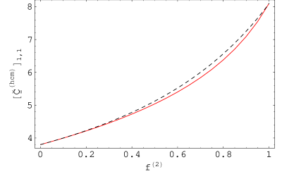
Refer to caption
Refer to caption
Refer to caption
Figure 1: Plots of [𝐂¯¯˘(hcm)]1,1subscriptdelimited-[]superscript˘¯¯𝐂𝑐𝑚11\left[\,\breve{\underline{\underline{\bf C}}}^{(hcm)}\,\right]_{1,1} (in GPa), [𝐂¯¯˘(hcm)]1,12subscriptdelimited-[]superscript˘¯¯𝐂𝑐𝑚112\left[\,\breve{\underline{\underline{\bf C}}}^{(hcm)}\,\right]_{1,12} (in C m-2) and (1/ϵ0)[𝐂¯¯˘(hcm)]12,121subscriptitalic-ϵ0subscriptdelimited-[]superscript˘¯¯𝐂𝑐𝑚1212(1/\epsilon_{\scriptscriptstyle 0})\left[\,\breve{\underline{\underline{\bf C}}}^{(hcm)}\,\right]_{12,12} as estimated using the lowest–order SPFT (i.e., hcm=ocm𝑐𝑚𝑜𝑐𝑚hcm=ocm) (black, dashed curves) and the Mori–Tanaka formalism (i.e., hcm=MT𝑐𝑚𝑀𝑇hcm=MT) (red, solid curves), versus the volume fraction of component material ‘2’. Component material ‘1’ is PVDF and component material ‘2’ is LaRC-SI, as described in §3.1. The component materials are distributed as spheres (i.e., a=b=c𝑎𝑏𝑐a=b=c).
Refer to caption
Refer to caption
Refer to caption
Figure 2: As Fig. 1 but with the component materials distributed as ellipsoids with (a/c=5𝑎𝑐5a/c=5 and b/c=1.5𝑏𝑐1.5b/c=1.5).
Refer to caption
Refer to caption
Refer to caption
Figure 3: As Fig. 1 but with the component materials distributed as ellipsoids with (a/c=10𝑎𝑐10a/c=10 and b/c=2𝑏𝑐2b/c=2).
Refer to caption
Refer to caption
Refer to caption
Refer to caption
Refer to caption
Refer to caption
Figure 4: Plots of the real and imaginary parts of the second–order SPFT estimates [𝐂¯¯~(spft)]1,1subscriptdelimited-[]superscript~¯¯𝐂𝑠𝑝𝑓𝑡11\left[\,\tilde{\underline{\underline{\bf C}}}^{(spft)}\,\right]_{1,1} (in GPa), [𝐂¯¯~(spft)]1,12subscriptdelimited-[]superscript~¯¯𝐂𝑠𝑝𝑓𝑡112\left[\,\tilde{\underline{\underline{\bf C}}}^{(spft)}\,\right]_{1,12} (in C m-2) and (103/ϵ0)[𝐂¯¯~(spft)]12,12superscript103subscriptitalic-ϵ0subscriptdelimited-[]superscript~¯¯𝐂𝑠𝑝𝑓𝑡1212(10^{3}/\epsilon_{\scriptscriptstyle 0})\left[\,\tilde{\underline{\underline{\bf C}}}^{(spft)}\,\right]_{12,12}, where 𝐂¯¯~(spft)=𝐂¯¯˘(spft)𝐂¯¯˘(ocm)superscript~¯¯𝐂𝑠𝑝𝑓𝑡superscript˘¯¯𝐂𝑠𝑝𝑓𝑡superscript˘¯¯𝐂𝑜𝑐𝑚\tilde{\underline{\underline{\bf C}}}^{(spft)}=\breve{\underline{\underline{\bf C}}}^{(spft)}-\breve{\underline{\underline{\bf C}}}^{(ocm)}, versus k¯L¯𝑘𝐿\bar{k}L, with f(2)=0.5superscript𝑓20.5f^{(2)}=0.5. The results from the spherical particle (i.e., a=b=c=1𝑎𝑏𝑐1a=b=c=1) case (red, solid line) are plotted alongside the cases with elliptical particles with a=5𝑎5a=5, b=1.5𝑏1.5b=1.5, c=1𝑐1c=1 (blue, short-dashed line) and a=10𝑎10a=10, b=2𝑏2b=2, c=1𝑐1c=1 (black, long-dashed line). Component material ‘1’ is PVDF and component material ‘2’ is LaRC-SI, as described in §3.1.
Refer to caption
Refer to caption
Figure 5: As Fig. 4 but with the real and imaginary parts of [𝝆¯~¯(spft)]11subscriptdelimited-[]superscriptbold-¯bold-¯bold-~𝝆𝑠𝑝𝑓𝑡11\left[\,\mbox{\boldmath$\underline{\underline{\bf\tilde{\rho}}}$}^{(spft)}\,\right]_{11} (in kg m-3), where 𝝆¯~¯(spft)=𝝆¯˘¯(spft)𝝆¯˘¯(ocm)superscriptbold-¯bold-¯bold-~𝝆𝑠𝑝𝑓𝑡superscriptbold-¯bold-¯bold-˘𝝆𝑠𝑝𝑓𝑡superscriptbold-¯bold-¯bold-˘𝝆𝑜𝑐𝑚\mbox{\boldmath$\underline{\underline{\bf\tilde{\rho}}}$}^{(spft)}=\mbox{\boldmath$\underline{\underline{\bf\breve{\rho}}}$}^{(spft)}-\mbox{\boldmath$\underline{\underline{\bf\breve{\rho}}}$}^{(ocm)}, plotted as functions of k¯L¯𝑘𝐿\bar{k}L, with f(2)=0.5superscript𝑓20.5f^{(2)}=0.5.