Alignment between galaxies and large-scale structure

Abstract

Based on the Sloan Digital Sky Survey DR6 (SDSS) and Millennium Simulation (MS) we investigate the alignment between galaxies and large-scale structure. For this purpose we develop two new statistical tools, namely the alignment correlation function and the $\cos(2\theta)$-statistic. The former is a two-dimensional extension of the traditional two-point correlation function and the latter is related to the ellipticity correlation function used for cosmic shear measurements. Both are based on the cross correlation between a sample of galaxies with orientations and a reference sample which represents the large-scale structure. We apply the new statistics to the SDSS galaxy catalog. The alignment correlation function reveals an overabundance of reference galaxies along the major axes of red, luminous ($L\gtrsim L_{\ast}$) galaxies out to projected separations of $60{\>h^{-1}\rm Mpc}$. The signal increases with central galaxy luminosity. No alignment signal is detected for blue galaxies. The $\cos(2\theta)$-statistic yields very similar results. Starting from a MS semi-analytic galaxy catalog we assign an orientation to each red, luminous and central galaxy, based on that of the central region of the host halo (with size similar to that of the stellar galaxy). As an alternative we use the orientation of the host halo itself. We find a mean projected misalignment between a halo and its central region of $\sim 25^{\circ}$. The misalignment decreases slightly with increasing luminosity of the central galaxy. Using the orientations and luminosities of the semi-analytic galaxies we repeat our alignment analysis on mock surveys of the MS. Agreement with the SDSS results is good if the central orientations are used. Predictions using the halo orientations as proxies for central galaxy orientations overestimate the observed alignment by more than a factor of 2. Finally, the large volume of the MS allows us to generate a two-dimensional map of the alignment correlation function which shows the reference galaxy distribution to be flattened parallel to the orientations of red luminous galaxies with axis ratios of $\sim 0.5$ and $\sim 0.75$ for halo and central orientations, respectively. These ratios are almost independent of scale out to $60{\>h^{-1}\rm Mpc}$.

1 Introduction

Recent large redshift surveys, like the 2dF Galaxy Redshift Survey (2dFGRS, Colless et al. 2001) and the Sloan Digital Sky Survey (SDSS, York et al. 2000), allow the cosmic large-scale density field to be traced with unprecedented accuracy. Different structures can reliably be classified as groups, filaments, walls and voids and match well with the patterns seen in N-body simulations. These structures induce large-scale tidal fields which in turn cause large-scale correlations in the orientations of massive dark matter halos (cf. Bond et al. 1996; Colberg et al. 1999; Altay et al. 2006) . However, the orientations of dark matter halos are difficult to observe. One needs either X-ray observations for a sufficient number of groups and clusters of galaxies or reliable galaxy-group catalogs derived from the redshift surveys. The former are expensive and the latter are prone to a number of systematic errors. Despite these difficulties both approaches have been pursued. In most cases alignment signals out to, at least, $20{\>h^{-1}\rm Mpc}$ have been found (Binggeli 1982; Ulmer et al. 1989; West 1989b; Plionis 1994; Chambers et al. 2000; Hashimoto et al. 2007). Instead of measuring the large-scale alignment based on groups and clusters of galaxies we suggest here to use directly the orientations of luminous galaxies and we quantify their alignment relative to large-scale structure.

Galaxies are not oriented at random. Rather, they have been found to show various forms of spatial alignment: between neighboring clusters of galaxies Binggeli (1982); West (1989a); Plionis (1994), between brightest cluster galaxies (BCGs) and their parent clusters Carter & Metcalfe (1980); Binggeli (1982); Struble (1990); Hashimoto et al. (2008), between the orientation of satellite galaxies and the orientation of the cluster Dekel (1985); Plionis et al. (2003), and between the orientation of satellite galaxies and the orientation of the BCG Struble (1990).

Observationally, these alignments are quantified either by the differential, $P(\theta)$, or cumulative, $P(\theta\leq\theta_{\rm max})$, probability distribution of the alignment angle $\theta$ which is the angle between the major axis of a galaxy and the line connecting it to a neighboring galaxy. Also the mean values of those distributions, $\langle\theta\rangle(r_{p})$, have been studied as a function of projected separation $r_{p}$. With recent large redshift surveys, in particular the SDSS, it has become possible to determine the alignment using large and homogeneous samples. Studies based on these surveys have focused mainly on the alignment of galaxies in groups. They revealed that satellite galaxies are preferentially distributed along the major axis of the central galaxies Brainerd (2005); Yang et al. (2006); Azzaro et al. (2007); Faltenbacher et al. (2007), and satellite galaxies tend to be preferentially oriented toward the central galaxy Pereira & Kuhn (2005); Agustsson & Brainerd (2006); Faltenbacher et al. (2007). Donoso et al. (2006) analyzed a high-redshift sample ($0.4<z<0.5$) of luminous red galaxies (LRGs) extracted from the SDSS, and found a clear signal of alignment between LRG major axes and the distribution of galaxies within $1.5h^{-1}$Mpc, indicating that the alignment effects observed in the local Universe were already present at $z\sim 0.5$.

In this paper we propose two new statistics to quantify the alignment between galaxies and the large-scale structure. The first one we call the alignment two-point correlation function which is an extension of the traditional two-point correlation function. Basically, the correlation is measured as a function of pair separation and alignment angle. The second measure we call $cos(2\theta)$-statistic and involves determining the mean cosine of twice the alignment angle for correlated pairs of given projected separation. We measure these statistics for SDSS galaxies as well as for semi-analytic galaxies within the Millennium simulation (MS) (Springel et al. 2005; De Lucia & Blaizot 2007), where the orientations of the semi-analytic galaxies are inferred from the orientation of their parent dark matter halos. The application of the new statistics reveals an alignment between red galaxies and large-scale structure out to $60{\>h^{-1}\rm Mpc}$.

The paper is organized as follows. In § 2 we introduce the two statistics used here to quantify the alignment between galaxies and large-scale structure. The statistics are applied to the SDSS galaxy catalog in § 3 and compared to the results derived from the semi-analytic galaxy catalog of the MS in § 4. Finally, § 5 gives a short summary.

2 Methodology

For the subsequent analysis we introduce two new statistical measures to quantify the correlations between galaxy orientations and the cosmic density field. The first quantity we call the alignment (two-point) correlation function, $w_{p}(\theta_{p},r_{p})$, where $\theta_{p}$ is the angle between the major axis of a galaxy and the connecting line to another one and $r_{p}$ is the projected separation between the two galaxies. This quantity is a two-dimensional extension of the traditional two-point projected correlation function. Paz et al. (2008) have used a related technique to analyze large-scale angular momentum alignments. The second quantity we refer to as the $cos(2\theta)$-statistic. This statistic is closely related to similar quantities used in the context of cosmic shear surveys. We compute both statistics only in projected space, i.e. orientations and pair separations are two-dimensional vectors. We keep this restriction also in the second part of this analysis where we compare observational and numerical results.

2.1 Alignment correlation function

The two-point correlation function (2PCF) has long served as the primary way of quantifying the clustering properties of galaxies in redshift surveys (e.g. Peebles 1980). It is defined as a function of pair separation by

$$dP_{12}=\bar{n}^{2}[1+\xi({\mathbf{r}})]dV_{1}dV_{2},$$ (1)

where $\xi({\mathbf{r}})$ is the 2PCF, $\bar{n}$ the mean number density of galaxies, and $dV_{1}$ and $dV_{2}$ are two infinitesimal volume elements centered at ${\mathbf{x}}_{1}$ and ${\mathbf{x}}_{2}$ with separation ${\mathbf{r}}={\mathbf{x}}_{2}-{\mathbf{x}}_{1}$. To be consistent with homogeneity and isotropy $\xi$ has been written as a function of the separation alone, that is, $\xi(r)$. If $\xi(r)\neq 0$, then galaxies are said to be clustered. As the fundamental second-order statistic of the density field, $\xi$ is simple to compute and provides a full statistical description for a Gaussian random field Bardeen et al. (1986). It can also be easily compared with the predictions of theoretical models (e.g. Aarseth et al. 1979; Davis et al. 1985). The amplitude of the correlation function on scales larger than a few Mpc provides a direct measure of the mass of the dark matter halos that host the galaxies through the halo mass-bias relation (e.g. Mo & White 1996; Jing et al. 1998).

In galaxy redshift surveys, the 2PCF is measured in redshift space and expressed either as a function of redshift-space separation $s$, giving rise to a 2PCF of $\xi(s)$, or as functions of separations perpendicular ($r_{p}$) and parallel ($\pi$) to the line of sight, giving rise to $\xi(r_{p},\pi)$ with $s^{2}=\pi^{2}+r_{p}^{2}$. In many cases, the projected 2PCF, $w_{p}(r_{p})$, is the more useful quantity, as it does not suffer from redshift-space distortions, and is thus directly related to the real-space correlation function $\xi(r)$. One can distinguish between two kinds of two-point correlation functions: two-point auto-correlation functions for which both members of a pair come from the same sample, and two-point cross-correlation functions (2PCCFs) for which the two members of a pair are from two different samples. In this paper we focus on the latter. In addition our analysis will be pursued in projected space, i.e. we focus on the projected 2PCCF $w_{p}(r_{p})$ where $r_{p}$ denotes the projected separation of a galaxy pair.

Given a sample of galaxies in question (Sample $Q$), a sample of reference galaxies (Sample $R$), and a random sample (Sample $\mathcal{R}$) that has the same selection function (i.e. distribution of redshifts and positions on the sky) as the reference sample, $\xi(r_{p},\pi)$ between $Q$ and $R$ can be estimated by

$$\xi(r_{p},\pi)=\frac{N_{\mathcal{R}}}{N_{R}}\frac{QR(r_{p},\pi)}{Q\mathcal{R}(r_{p},\pi)}-1,$$ (2)

where $N_{R}$ and $N_{\mathcal{R}}$ are the number of galaxies contained in the reference and random samples, with $N_{\mathcal{R}}/N_{R}=10$ throughout this paper. $QR(r_{p},\pi)$ and $Q\mathcal{R}(r_{p},\pi)$ are the counts of cross pairs between the indicated samples for a given separation perpendicular, $r_{p}$, and parallel, $\pi$, to the line-of-sight. With the measurement of $\xi(r_{p},\pi)$ in hand one can then estimate the projected cross-correlation function $w_{p}(r_{p})$ by integrating $\xi(r_{p},\pi)$ along the $\pi$ direction:

$$w_{p}(r_{p})=\int_{-\pi_{\rm max}}^{+\pi_{\rm max}}\xi(r_{p},\pi)d\pi=\sum_{i}\xi(r_{p},\pi_{i})\Delta\pi_{i},$$ (3)

where $\pi_{\rm max}$ has to be sufficiently large to minimize the probability of erroneously excluding correlated pairs with line-of-sight separations larger than $\pi_{\rm max}$.

Now we extend the definition of the 2PCCFs, so that they will be able to quantify the spatial alignment of galaxies. For each pair of galaxies with one member from Sample $Q$ (the main galaxy) and the other from Sample $R$ (the reference galaxy), we consider $\theta_{p}$, the angle between the major axis of the main galaxy and the line connecting the two galaxies projected onto the sky. We include this angle as a second property of the pair, in addition to the pair separation. In this case, the correlation function is not only a function of the projected separations, but also of $\theta_{p}$. The estimator of Eq. (4) is easily modified to account for the dependence on $\theta_{p}$:

$$\xi(\theta_{p},r_{p},\pi)=\frac{N_{\mathcal{R}}}{N_{R}}\frac{QR(\theta_{p},r_{p},\pi)}{Q\mathcal{R}(\theta_{p},r_{p},\pi)}-1,$$ (4)

$QR(\theta_{p},r_{p},\pi)$ and $Q\mathcal{R}(\theta_{p},r_{p},\pi)$ are the counts of cross pairs between the indicated samples for given $\theta_{p}$, $r_{p}$ and $\pi$. The projected correlation function is found by integration along the line-of-sight.

$$w_{p}(\theta_{p},r_{p})=\int_{-\pi_{\rm max}}^{+\pi_{\rm max}}\xi(\theta_{p},r_{p},\pi)d\pi=\sum_{i}\xi(\theta_{p},r_{p},\pi_{i})\Delta\pi_{i}$$ (5)

The traditional correlation function is just the average of the new correlation function over the full range of $\theta_{p}$ values. Taking symmetries into account the value of the angle ranges from zero (along the major axis of the main galaxy) to 90 degrees (perpendicular to the major axis). Thus, higher amplitudes of the new correlation functions at small values of $\theta_{p}$ indicate that the reference galaxies are more likely to be aligned along the major axis of the main galaxies. In contrast, higher amplitudes at larger angles indicate that the reference galaxies are more likely to be located along the minor axis of the main galaxies. This new statistic can be used for quantifying the alignment of galaxies and we refer to it as the alignment correlation function.

On small scales ($\la$ Mpc), this statistic can be used to confirm the alignment between central and satellite galaxies in groups and clusters, if Sample $Q$ consists purely of central galaxies (cf. Carter & Metcalfe 1980; Binggeli 1982; Struble 1990). More interestingly, the new statistic allows us to extend the alignment study to very large scales without worrying about selection effects, which are taken into account by comparison with the random sample ($\mathcal{R}$). On large scales, this statistic can be used to quantify the alignment of the main galaxies (which may or may not be central galaxies) with respect to the large-scale structure of the Universe as probed by the large-scale distribution of the reference galaxies.

As the final remark of this section we would like to mention that one can easily derive equivalent expressions for the alignment auto-correlation function – additionally it is straightforward to extend the formalism to three dimensional problems.

2.2 The $\cos(2\theta)$-statistic

The $\cos(2\theta)$-statistic gives the average of $\cos(2\theta_{p})$ for all correlated pairs at a given projected separation. It will be referred as ${\langle\cos(2\theta_{p})_{cor}\rangle}(r_{p})$ where the index $cor$ emphasizes that the average is based on correlated pairs only. Again, $\theta_{p}$ indicates the angle between the major axis of a main galaxy and the line connecting it with a reference galaxy. More precisely, using the alignment correlation function, $w_{p}(\theta_{p},r_{p})$, we define

$${\langle\cos(2\theta_{p})_{cor}\rangle}(r_{p})={\int_{0}^{\pi/2}\cos(2\theta_{p})w_{p}(\theta_{p},r_{p})d\theta_{p}\over\int_{0}^{\pi/2}w_{p}(\theta_{p},r_{p})d\theta_{p}}\ .$$ (6)

This statistic is constrained to values between $-1$ and $1$. Values above and below 0 indicate a preference for small ($<45^{\circ}$) and large ($>45^{\circ}$) angles, respectively. Values close to 0 are expected for isotropy. An estimator for Eq. 6 is given by

$${\langle\cos(2\theta_{p})_{cor}\rangle}(r_{p})={\sum_{i}\left({QR_{\theta}(r_{p},\pi_{i})\over Q\mathcal{R}(r_{p},\pi_{i})}\right)\Delta\pi_{i}\over\sum_{i}\left({QR(r_{p},\pi_{i})\over Q\mathcal{R}(r_{p},\pi_{i})}-1\right)\Delta\pi_{i}}\ ,$$ (7)

where $QR_{\theta}(r_{p},\pi_{i})$ symbolizes the sum of $\cos(2\theta_{p})$ for all cross pairs between main and reference samples ($Q$ and $R$) within the given separation bins, $r_{p}$ and $\pi_{i}$. As before, $QR(r_{p},\pi_{i})$ and $Q\mathcal{R}(r_{p},\pi_{i})$ denote the number of cross pairs between the indicated samples for $r_{p}$ and $\pi_{i}$.

Related statistics are used in weak lensing studies where they are referred to as ellipticity correlations (e.g. Miralda-Escude 1991; Croft & Metzler 2000; Heavens et al. 2000). In particular we want to point out the similarity to the the intrinsic shear-density correlation function $w_{g+}(r_{p})$ (Mandelbaum et al. 2006; Hirata et al. 2007) which measures the correlation between galaxy orientations and the large-scale density distribution. Leaving the ellipticity weighting and ‘responsivity’ correction aside (cf. Eqs. 8 and 9 in  Hirata et al. 2007) the following relation holds.

$$\tilde{w}_{g+}=w_{p}(r_{p}){\langle\cos(2\theta_{p})\rangle}_{cor}(r_{p})$$ (8)

where $\tilde{w}_{g+}$ indicates the unweighted version of $w_{g+}$. We do not weight by ellipticity since we here are solely interested in the spatial alignment between galaxies and the large-scale structure.

3 Alignment of SDSS galaxies

In this section we apply the two new statistics to the publicly available data from the Sloan Digital Sky Survey DR6. Before doing that we describe some details of the survey and the galaxy sample construction. Also the determination of the galaxy orientations is reviewed.

3.1 Galaxy sample construction

The observational data used in this paper are taken from the SDSS which has been designed to obtain photometry of a quarter of the sky and spectra of nearly one million objects. Imaging is obtained in the u, g, r, i, z bands Fukugita et al. (1996); Smith et al. (2002); Ivezić et al. (2004). The details of the survey strategy can be found in York et al. (2000) and an overview of the data pipelines and products is provided in the Early Data Release paper Stoughton et al. (2002). The SDSS has had seven additional major data releases Abazajian et al. (2003, 2004, 2005); Adelman-McCarthy et al. (2006, 2007, 2008).

The galaxy samples for this work are constructed from Sample dr6 of the New York University Value Added Galaxy Catalogue (NYU-VAGC), which is based on the SDSS DR6, publicly available at http://sdss.physics.nyu.edu/vagc/. A detailed description thereof can be found in Blanton et al. (2005). Our sample consists of 430164 galaxies that are identified as galaxies from the Main sample (note that $r$-band magnitude has been corrected for foreground extinction), and are in the ranges of $0.01<z<0.4$, $-23<M_{{}^{0.1}r}<-17$ and $14.5<r<17.6$. Here $M_{{}^{0.1}r}$ is the $r$-band absolute magnitude corrected to its $z=0.1$ value using the $K-$correction code of Blanton et al. (2003b) and the luminosity evolution model of Blanton et al. (2003a). We do not consider galaxies fainter than $M_{{}^{0.1}r}=-17$, because the volume covered by such faint samples is very small and the results are subject to large errors as a result of cosmic variance (see for example Fig. 6 of Li et al. 2006). The faint apparent magnitude limit of 17.6 is chosen to yield an uniform galaxy sample that is complete over the entire area of the survey. This sample will serve as the reference sample (Sample $R$) for computing cross-correlation functions, as well as the parent sample for selecting different subsamples ($Q$).

The large amount of data allows us to split the parent sample into various subsamples. Thus, we split all the galaxies into 4 subsamples according to their $r$-band absolute magnitudes, ranging from $M_{{}^{0.1}r}=-23$ to $M_{{}^{0.1}r}=-17$ with an interval of 1 magnitude. Further, we classify each galaxy with $M_{{}^{0.1}r}>-22$ as either “red” or “blue” according to its $g-r$ color. To this end, we follow Li et al. (2006) to fit the $g-r$ distribution at fixed luminosity with a bi-Gaussian profile and use the mean of the two Gaussian centers as the color cut. In the highest luminosity bin, $-23<M_{{}^{0.1}r}<-22$, this color separation scheme is problematic, basically because the blue population is extremely sparse, thus we assign all galaxies within this magnitude bin to the red population (cf. Li et al. 2006, Fig. 9). These subsamples will be cross-correlated with the full parent sample, i.e. the reference sample.

To compute the cross-correlation function between the main and reference samples, $Q$ and $R$, one also needs to construct a random sample, $\cal R$, where galaxies with random coordinates are subject to the same selection effects as the reference sample. Since the reference sample is used as a tracer of the large-scale structure only the galaxy positions instead of their orientations are of interest. Accordingly, orientations are not considered when constructing the random sample. A detailed account of the selection effects accompanies the NYU-VAGC release Blanton et al. (2005) which is the base for the construction of the random sample used here (cf. Li et al. 2006).

3.2 Determination of galaxy orientations

The orientation of galaxies is quantified by the position angle (PA) of the major axis of their $r$-band images, which is determined by the SDSS photometric pipeline called Photo Lupton et al. (2001). Photo provides three quantities for the PA of each galaxy: PA_deV, PA_exp, and PA_iso. The first two come from fitting two models to the two-dimensional image of the galaxy in each band: a pure de Vaucouleurs profile and a pure exponential profile, while the last one is given by measuring the shape parameters (centroid, major and minor axes, PA, and average radius) of the 25 mag arcsec^-2 isophote. Details on the photometric pipeline can be found in Lupton et al. (2001) and Stoughton et al. (2002). In this paper we use the isophotal PA, PA_iso. However, we found no significant variation in the alignment signals when adopting the alternative definitions for the PAs.

To quantify the intrinsic scatter of the alignment signal we randomly shuffle the PAs among the galaxies in the main sample and redo the alignment analysis. Since the shuffled orientations are not correlated with the large-scale structure one expects no systematic alignment signal. The $1\sigma$ variance of 10 randomly shuffled samples can then be used to infer the intrinsic scatter.

3.3 Alignment correlation function

Figure 1: Upper panels in each set: Solid lines display the projected SDSS alignment correlation function, $w_{p}(\theta_{p},r_{p})$, between our reference sample and red (upper set) and blue (lower set) main galaxies in different intervals of $r$-band absolute magnitude. The colors correspond to three ranges in $\theta_{p}$ as indicated. The dashed black line shows the conditional correlation function averaged over angle. Lower panels in each set: Ratio between the angle dependent correlation functions and their mean. The color code is the same as used in the upper panels. The shaded regions plotted in red, green and blue colors indicate the $1-\sigma$ variance based on 10 samples in which the position angles are shuffled at random among the galaxies. By definition (§ 3.1) there are no blue galaxies in the brightest luminosity bin so these panels are kept void.

We now compute the alignment correlation function, $w_{p}(\theta_{p},r_{p})$, based on Eq. 5 with $\pi_{\rm max}=40{\>h^{-1}\rm Mpc}$. We probe projected separations up to $60{\>h^{-1}\rm Mpc}$ within three angular bins. A less coarse angular binning is prohibited by Poisson noise at large separations.

3.3.1 Alignment for red galaxies

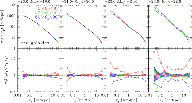
The first row of the upper panel of Fig. 1 shows the alignment correlation function for red galaxies in various magnitude bins. The red, green and blue solid lines display the results for the different angular bins, $0^{\circ}-30^{\circ}$, $30^{\circ}-60^{\circ}$ and $60^{\circ}-90^{\circ}$, respectively. The low angle bin, $0^{\circ}-30^{\circ}$, quantifies the correlation function along the orientation of the main galaxies. The $60^{\circ}-90^{\circ}$ bin contains information about the reference galaxy abundance perpendicular to the orientation of the main galaxies. The long dashed black line represents the traditional correlation function and is a weighted average of the three bins.

The second row of the upper panel of Fig. 1 shows the ratio of the alignment correlation function to the traditional one. The color code is the same as used in the row above. The shaded regions indicate the $1\sigma$ variance between 10 random samples in which the orientations are shuffled at random among the galaxies. A signal well outside the shaded region is a significant detection of alignment or anti-alignment depending on whether the signal lies above or below one.

The alignment correlation functions (colored lines) for red galaxies in the lowest luminosity bin ($-20<M_{{}^{0.1}r}<-19$) can hardly be distinguished from the traditional correlation function (dashed black line). However, the corresponding ratio, $w_{p}(\theta_{p},r_{p})/w_{p}(r_{p})$, shows a weak but systematic trend to anisotropy at scales larger than $\sim 10{\>h^{-1}\rm Mpc}$. At these separations the reference galaxies are preferentially located along the major axes of the main galaxies. Along the minor axes the reference galaxies are correspondingly under-abundant. This feature becomes more pronounced in higher luminosity bins. For galaxies brighter than $M_{{}^{0.1}r}=-20$ a significant overabundance of reference galaxies is visible along the major axis. The signal reaches from $10{\>h^{-1}\rm kpc}$ out to $60{\>h^{-1}\rm Mpc}$ which corresponds the entire range probed here.

These plots indicate that the orientations of red galaxies are connected to the large-scale structure in which they are embedded. Any realistic galaxy formation model should be able to reproduce this interlacing between dimensions spanning $\sim 3$ orders of magnitude.

3.3.2 Alignment for blue galaxies

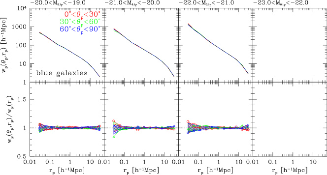
The lower panels of Fig. 1 display the corresponding results for blue galaxies. Otherwise the analysis is carried out in exactly the same manner as for the red galaxies. The panel for the highest magnitude bin, $-23<M_{{}^{0.1}r}<-22$, is left void because by definition there are no blue galaxies with these luminosities (see § 3.1). In the lower three magnitude bins we do not find any indication for alignment between the galaxies and the reference galaxy distribution. The differences seen between red and blue galaxies suggest that the orientations of red and blue galaxies are determined by distinct physical processes.

3.4 $\cos(2\theta)$-statistic

In this section we compute the $\cos(2\theta)$ statistic based on the same subdivision of the parent SDSS sample by color and $r$-band absolute magnitude as used above for the alignment correlation function. In a second step we focus on the alignment signal for group central galaxies. This is to facilitate a comparison with simulation results discussed in the second part of this paper.

3.4.1 Color and luminosity dependence

Figure 2: $\cos(2\theta_{p})$ statistic for SDSS data. The results for red and blue main galaxies are displayed by red and blue lines. The galaxies are subdivided into four $r$-band absolute magnitude bins as indicated. The shaded regions in red and blue show the $1\sigma$ variance between 10 random samples in which the position angles are shuffled at random among the main galaxies. The reference sample is the same for all these measurements and comprises all galaxies with $r$-band absolute magnitudes in $-23<M_{{}^{0.1}r}<-17$. No results are shown for blue galaxies in the highest luminosity since, by definition, they are red galaxies.

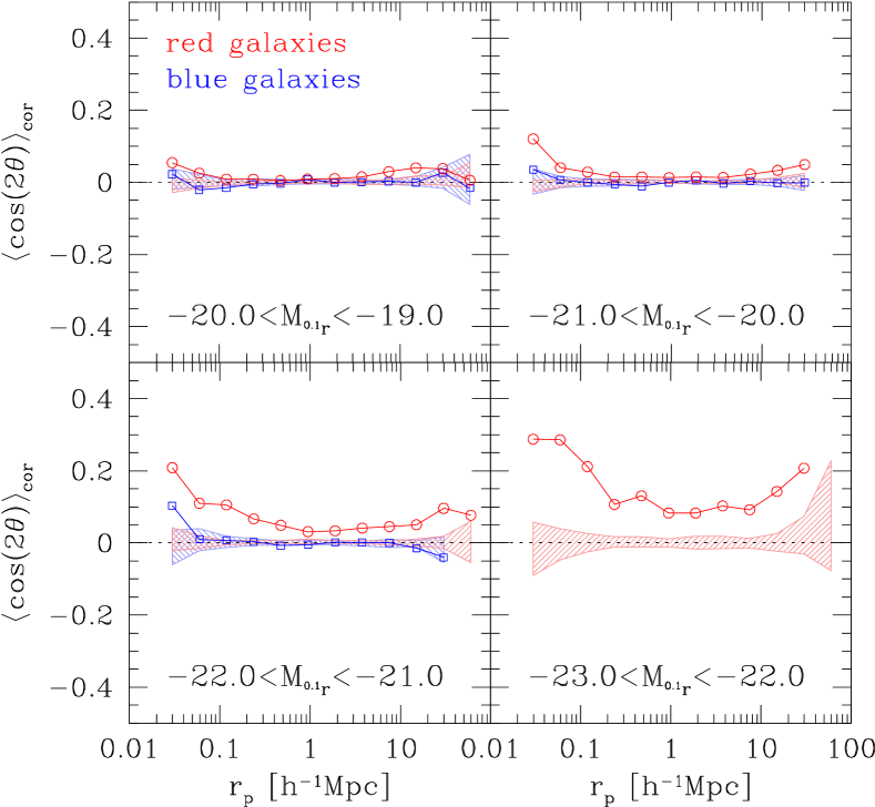
Fig. 2 displays the $\cos(2\theta_{p})$-statistic as discussed in § 2.2. The results for red and blue galaxies are displayed by red and blue lines. The shaded regions show the $1\sigma$ variance between the 10 random samples. The signal for the red galaxies shows a strong dependence on luminosity. There is basically no signal for red galaxies in the lowest luminosity bin. For $r$-band absolute magnitudes, ranging from $M_{{}^{0.1}r}=-20$ to $M_{{}^{0.1}r}=-23$ the signal systematically lies above the shaded region, indicating that it can not be explained by the intrinsic scatter inherent to the data. The signal is significant on all scales probed ($\leq 60{\>h^{-1}\rm Mpc}$) and becomes more pronounced with increasing luminosity. Blue galaxies do not show any indication for alignment with the reference galaxy distribution. Fig. 2 suggests that red galaxies with $L\gtrsim L_{\ast}$ tend to be aligned with large-scale structure out to at least $60{\>h^{-1}\rm Mpc}$. This result is very similar to that from the alignment correlation function discussed in § 3.3. It supports the picture of a physically distinct origin for the orientations of red and blue galaxies.

3.4.2 Alignment of group central galaxies

Figure 3: $\cos(2\theta_{p})$ statistic for SDSS central galaxies. See the text for our definition of ‘central’. Results for red and blue galaxies are displayed by red and blue lines. All symbols are the same as used in Fig. 2.

Alignment between clusters of galaxies has been detected out to large scales $\sim 100{\>h^{-1}\rm Mpc}$) (e.g., Binggeli 1982; Plionis 1994; Hashimoto et al. 2007). In addition there exists strong evidence that the orientations of central galaxies are aligned with the orientations of their parent groups or clusters. Now the question arises whether an exclusion of non-central galaxies may enhance the alignment signal measured before. To this end we redo the above analysis excluding non-central galaxies. This approach also facilitates a subsequent comparison with N-body results, since there only the orientations of central galaxies are available (see § 4.4).

Central galaxies are found in the following way. For each main galaxy, we use its $r$-band absolute magnitude to calculate a halo mass, according to the relation between central galaxy luminosity and halo mass as given by Yang et al. (2005a). We then estimate a ‘virial’ radius using the model of Eke et al. (2001). We find all the companions around the galaxy within this radius and a line of sight velocity separation of $\pm 3000\>{\rm km}\,{\rm s}^{-1}$ and compare the luminosity of the galaxy to that of the companions. If the galaxy is brighter than any of its companions and it is not inside the virial radius of a farther, brighter galaxy it is classified as a ‘central’ galaxy. Otherwise, it is a ‘non-central’ galaxy. This method will inevitably mis-judge a certain fraction of galaxies to be non-central due to the appearance of more luminous interlopers (cf. Yang et al. 2005b). However, it should be sufficient to estimate the signal for central galaxies. This can then be compared to the signal for the complete sample as well as to simulations.

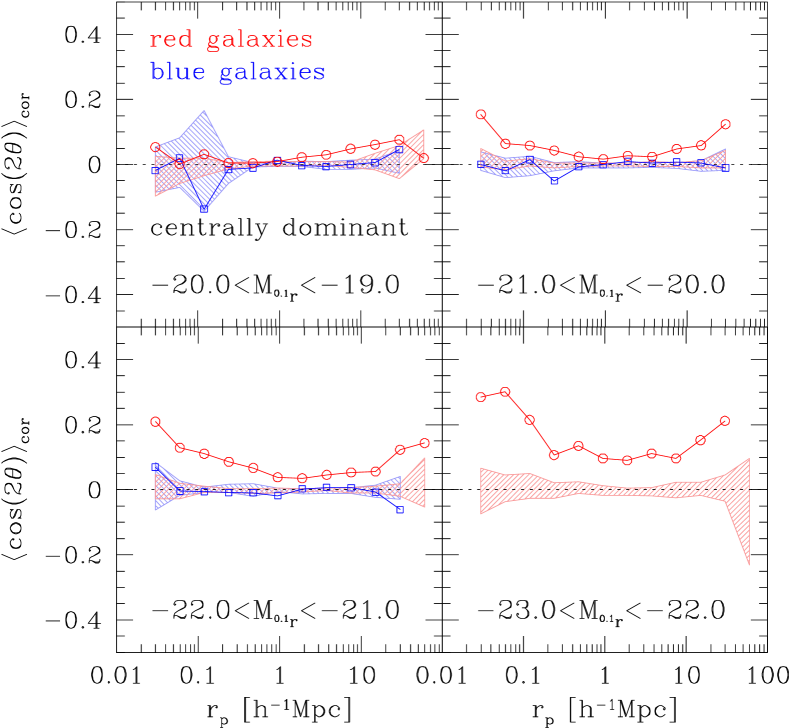
Fig. 3 displays the alignment signals based on central galaxies only. As before we do not find any alignment signal for blue galaxies. The upper two luminosity bins show only marginal differences when compared to the complete sample. This can be explained by the fact that most bright galaxies are central. For the lower two luminosity bins the alignment signal increases by a few per cent which indicates a certain reduction of the alignment signal for the complete sample which includes non-central galaxies (Fig. 2). We come to the conclusion that the alignment signal is not strongly enhanced by the exclusion of non-central galaxies which is due in part to the fact that luminous galaxies usually are central.

4 Comparison to the alignment of MS galaxies

In the second part of this study we apply our new analysis tools (alignment correlation function and $\cos(2\theta$)-statistic) to semi-analytic galaxies in the MS. Orientations have to be assigned to the model galaxies and we investigate different approaches, comparing the resulting alignment signals with the observed ones. Since we did not detect any alignment signal for blue galaxies we restrict our orientation assignment to red model galaxies. This restriction may also be justified by a slightly different kind of reasoning. Namely, red luminous galaxies are predominantly elliptical galaxies. Those are thought to form via merging of proto-galaxies which is basically a collisionless process. Thus N-body simulations may be able to recover some characteristic features of red galaxies, in particular their orientation. Blue galaxies, on the other side, are mainly spiral galaxies with their properties heavily dependent on baryonic, i.e. collisional, physics. Thus their properties may be only poorly recovered by N-body simulations. This picture may change at high redshifts. At that time, also the orientation of many blue galaxies could be a product of gas-rich mergers.

In the following two paragraphs we list some details of the MS and describe how we estimate orientations for the model galaxies. Subsequently we redo the analysis already carried out on SDSS galaxy samples and we compare the results.

4.1 The simulation and the galaxy sample

The Millennium Simulation (Springel 2005) adopted concordance values for the parameters of a flat $\Lambda$ cold dark matter ($\Lambda$CDM) cosmological model, $\Omega_{\rm dm}=0.205$ and $\Omega_{\rm b}=0.045$ for the current densities in CDM and baryons, $h=0.73$ for the present dimensionless value of the Hubble constant, $\sigma_{8}=0.9$ for the rms linear mass fluctuation in a sphere of radius $8{\>h^{-1}\rm Mpc}$ Mpc extrapolated to $z=0$, and $n=1$ for the slope of the primordial fluctuation spectrum. The simulation followed $2160^{3}$ dark matter particles from z= 127 to the present day within a cubic region $500{\>h^{-1}\rm Mpc}$ on a side resulting in individual particle masses of $8.6\times 10^{8}{\>h^{-1}\rm M}_{\odot}$. The gravitational force had a Plummer-equivalent comoving softening of $5{\>h^{-1}\rm kpc}$. The Tree-PM $N$-body code GADGET2 (Springel et al. 2005) was used to carry out the simulation and the full data were stored 64 times spaced approximately equally in the logarithm of the expansion factor. This information makes it possible to construct trees that store detailed assembly histories for each dark matter halo present at z= 0.

The halos are found by a two-step procedure. In the first step all collapsed halos with at least 20 particles are identified using a friends-of-friends (FoF) group-finder with linking parameter b = 0.2. These objects will be referred to as FoF-halos. Then post-processing with the substructure algorithm SUBFIND (Springel et al. 2001) subdivides each FoF-halo into a set of self-bound sub-halos. Here we only consider the main sub-halo which is the sub-halo with the most massive progenitor among all sub-halos belonging to the same FoF-halo. We refer to this sub-halo as the parent sub-halo associated with the central galaxy.

Based on the assembly histories individual halos are populated with semi-analytic galaxies for which many ‘observable’ quantities are generated. For a detailed description of the construction of the semi-analytic galaxy catalog we refer the reader to Croton et al. (2006) and De Lucia & Blaizot (2007). Here we use the DeLucia2006a_SDSS2MASS catalog (http://www.g-vo.org/MyMillennium2/) which provides synthetic magnitudes through SDSS filters, alternatively to classify the model galaxies as well as to tag their parent sub-halos. The use of semi-analytic galaxies facilitates comparison to the observations and is also an elegant way to characterize the assembly history of the host halo by a few numbers.

$M_{r}$	$[-20,-19]$	$[-21,-20]$	$[-22,-21]$	$[-23,-22]$
$N_{\rm halo}$	16027	98618	167513	53065
${\langle N_{\rm sub}\rangle}$	489	1672	4707	18662
${\langle N_{\rm cen}\rangle}$	31	83	164	278

Table 1: Particle number statistics for host halos

Our standard reference sample comprises a random subset (1103640 galaxies) of all semi-analytic galaxies with $r$-band absolute magnitudes of $-23\leq M_{r}\leq-17$ (in total 11027979 galaxies) at $z=0$. This standard reference sample is used for all the subsequent analysis based on MS galaxies. The parent galaxy sample comprises all red, central galaxies within the same magnitude range as the reference galaxies ( $-23\leq M_{r}\leq-17$). A galaxy is red if $g-r\geq 0.7$, where $g$ and $r$ are synthetic magnitudes in the corresponding SDSS bands. A galaxy is central if it is the dominant galaxy in a given FoF-halo. Expressed in the MS terminology it is the (only) type 0 galaxy within this FoF-halo. This definition comes close to the selection we have employed to identify central galaxies in the observational analysis above. In analogy to the SDSS sample the MS galaxies are split into four $r$-band magnitude bins with equal intervals of one magnitude. Each model galaxy is associated with a dark matter halo which will be used to determine the orientation of the galaxy. For the four magnitude bins Table 1 lists: the number of halos ($N_{\rm halo}$); the average number of particles belonging to these halos, ${\langle N_{\rm sub}\rangle}$; and the average number of particles belonging to the central part of the halos, ${\langle N_{\rm cen}\rangle}$. The determination of the number of central particles is related to the computation of the central orientations and will be discussed below. We conclude this paragraph by emphasizing that orientations are only determined for red, central galaxies, because only for those galaxies do we expect a tight correlation between the orientations of galaxy and halo.

4.2 The orientations of semi-analytic galaxies

As a proxy for the major axis of the central galaxy we adopt the major axis of the projected moment of inertia tensor of the parent sub-halo (cf. Agustsson & Brainerd 2006; Kang et al. 2007; Faltenbacher et al. 2008; Knebe et al. 2008; Okumura et al. 2008). Since real galaxies are seen in projection, we project the dark matter distribution before diagonalizing the moment of inertia tensor. We determine the orientations of each central galaxy in two alternative ways. We use the dark matter distribution of the parent sub-halo, (i.e. the main sub-halo of the FoF-halo) or we only use its central part to approximate the orientation of the central galaxy. The former is done to compare the results to earlier work while the latter better mimics the true physical circumstance (cf. Faltenbacher et al. 2008; Knebe et al. 2008). We will refer to the former as halo orientation and the latter as central or galaxy orientation. The central orientation is determined in an iterative way. We begin by computing a number of central particles $N_{cen}$ using the following formula

$$N_{cen}=\begin{cases}37\ &\times\ N_{sub}^{0.2}\ \text{ for }N_{sub}\geq 4900\\ 0.225&\times\ N_{sub}^{0.8}\ \text{ for }N_{sub}<4900\end{cases}$$ (9)

where $N_{sub}$ is the number of particles within the parent sub-halo. This formula is a two-power-law approximation to the observed relation between the luminosity of a central galaxy and its parent halo mass (e.g. Cooray & Milosavljević 2005). It reflects the assumption that the distribution of a galaxy’s stellar component can be represented by the central matter distribution of its simulated dark matter halo. The mass representing the galaxy then has to follow the observed scaling laws. Now, let $r_{init}$ be the radius which encloses the $N_{cen}$. In a first iteration step the moment of inertia is computed within the $r_{init}$. The resulting axis ratios are used to cut out a central ellipsoidal where the length of the intermediate axis is fixed to $r_{init}$. Based on this new subset of particles the moment of inertia is computed anew. The iteration is continued until the central orientation converges. Fixing the intermediate axis results in approximately unchanging particle numbers within consecutive ellipsoids. Up to this point the computations were done in three dimensions. In a last step all particles within the final ellipsoid are projected onto the plane of the sky. The inertia tensor of this 2-D distribution determines the central orientation.

Figure 4: Probability distribution of the misalignment angle between halo and central (galaxy) orientations for a series of magnitude bins as indicated. Errors represent Poisson uncertainties. The small vertical lines on the bottom axis denote the mean values of the distributions. The dashed line display the result of Okumura et al. (2008) and its mean we show as black dashed mark on the bottom axis.

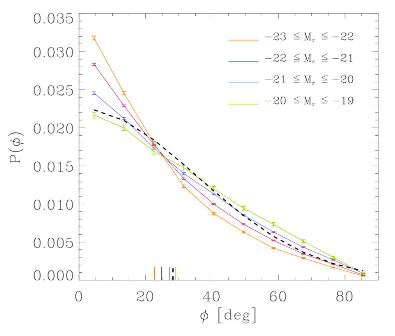
In Fig. 4 the difference between halo and central (galaxy) orientations are illustrated by the probability distribution function (PDF) of the misalignment angle between them. The mean values of the misalignment for each magnitude bin are indicated by the little vertical marks on the bottom axis. As indicated in Table 1, on average there are only 31 particles used to determine the central orientations within the lowest luminosity bin. Thus, Poisson noise adds an additional misalignment component which contributes to the flattening of the PDF at small angles. In fact calculating the misalignment using central volumes twice as large as given by Eq. 9 substantially reduces the flattening in the lowest luminosity bin. However, since we aim to probe the volume actually occupied by the stellar component of the galaxies we adhere to Eq. 9 keeping in mind that the central orientations for the low luminosity galaxies are poorly resolved. Such effects are less important for the higher luminosity bins. The two highest luminosity bins use 160 and 270 particles on average which should result in a robust determination of the orientations (cf. Jing 2002). For comparison we also display the Gaussian PDF suggested by Okumura et al. (2008), who found a mean misalignment angle of $\sim 25^{\circ}$ between the halo and the galaxy orientation. Comparing the orientations of central galaxies and their host halos a similar misalignment has been found by Agustsson & Brainerd (2006) and Kang et al. (2007). Somewhat lower values are quoted in Wang et al. (2008). The misalignment weakens slightly with increasing luminosity of the central galaxy, though this may be due to the resolution effects discussed above.

4.3 Alignment correlation function

With these orientations and the model magnitudes the alignment, correlation function can be computed for the galaxies in the MS. We will adopt the same luminosity bins used for our analysis of the SDSS data, simplifying the comparison between observations and simulations. For the computation of the alignment angle we apply the distant observer approximation. To that end the z-direction in the simulation is chosen to be parallel to the line of sight. To mimic the observational approach the maximum projected separation of pairs along the line of sight is $\pi_{\rm max}=40{\>h^{-1}\rm Mpc}$.

Figure 5: Upper panels: Projected MS alignment correlation function, $w_{p}(\theta_{p},r_{p})$, for red central galaxies in different intervals of $r$-band absolute magnitude using the standard reference sample. The colors correspond to the sectors as indicated. The solid and dashed lines are based on central and halo orientations. The dotted line represents the traditional projected two-point cross-correlation function, $w_{p}(r_{p})$. Lower panels: Ratio between the alignment and traditional correlation functions. The color code is the same as used above. Red and blue shaded regions indicate the $1-\sigma$ variance based on 10 samples in which the central orientations are shuffled at random among the galaxies.

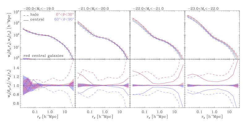
Fig. 5 shows the alignment correlation function for four luminosity bins which can be compared to the upper panel in Fig. 1. Also the luminosity range of the reference sample is chosen to be the same as in our observational analysis. At this point we would like to emphasize that the MS main sample only includes central galaxies. This causes the pronounced bend at a few hundred ${\>h^{-1}\rm kpc}$ corresponding roughly to virial radii of the host halos. The general behavior, however, is very similar to that seen in Fig. 1. The correlation function is enhanced along the major axes of the red galaxies ($0^{\circ}<\theta_{p}<30^{\circ}$) and reduced perpendicular to them. For galaxies brighter than $M_{r}\leq-20$ a systematic alignment/anti-alignment signal is seen over the entire separation range probed (out to $60{\>h^{-1}\rm Mpc}$). And the strength of the alignment effect increases with the luminosity of the galaxies.

In addition we find that, except for small (intra-halo) scales, the alignment signal based on the halo orientations is more pronounced than that based on the central (galaxy) orientations. This can be explained by the misalignment between halo and central orientations discussed in § 4.2. A comparison with the upper panel of Fig. 1 reveals that the alignment based on halo orientations overestimates the observational signal whereas that based on the central orientations reproduces the amplitudes obtained for SDSS galaxies quite well.

Figure 6: 2D alignment correlation function based on the DeLucia2006a_SDSS2MASS semi-analytic galaxy catalog for the MS. The main sample consists of red, central galaxies with absolute $r$-band magnitudes between $-21$ and $-22$. The orientations of the galaxies are aligned with the x-axis. Left and right panels display results based on halo and central orientations. Panels from top to bottom show the same distribution for different scales. The color code indicates the correlation amplitude, its range changes from top to bottom. Pixels with values below and above the indicated range are displayed black and yellow, respectively. The ratios of minor to major axes at $\log w_{p}(x,y)=1.5$, $1$ and $0.5$ are 0.57, 0.61 and 0.42 for the halo and 0.75, 0.80, 0.75 for the central orientations.

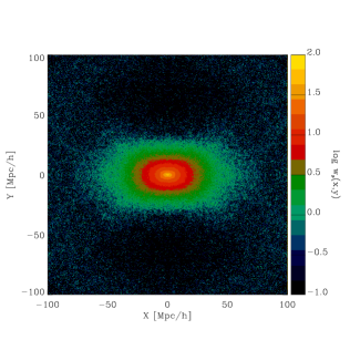
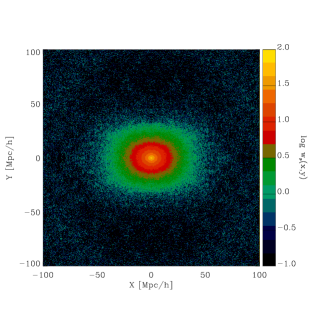
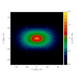
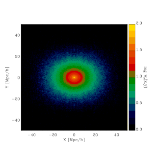
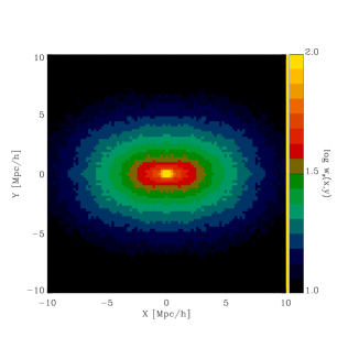
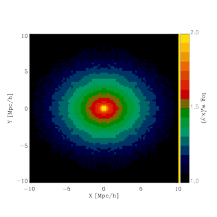
So far we have restricted the computation of the alignment correlation to 3 angular bins, a relatively coarse segmentation. This facilitates the direct comparison with the SDSS results, derived above, where a less coarse binning would result in excessive Poisson noise. However the MS provides much better statistics, making possible the computation of a 2D alignment correlation map as displayed in Fig. 6. This shows the alignment cross-correlation between a sample consisting of red ($g-r\geq 0.7$), central galaxies with $r$-band luminosities between -21 and -22 and our standard reference sample. The left and right panels are based on halo and central orientations, respectively. The panels in a column display consecutive blowups of the same map. The correlation amplitude can be read off using the adjacent color bars. Note, the range changes from top to bottom. The ratios of minor to major axes for $\log w_{p}(x,y)=1.5$, $1$ and $0.5$ are 0.57, 0.61 and 0.42 for the halo orientations and 0.75, 0.80, 0.75 for the central orientations. In agreement with the results above, the alignment correlation based on halo orientations is more anisotropic. It is striking that the flattening of the counts is almost constant over the range of scales we can measure.

The main conclusion to be drawn from Figs. 5 and 6 is that the halos of red luminous galaxies are aligned with the surrounding galaxy distribution out to at least $60{\>h^{-1}\rm Mpc}$. If the orientations of the galaxies are approximated by the orientation of the halos as a whole, the alignment signal is strong. The misalignment between the halo and central region, as discussed in § 4.2, causes a weakening of the correlation. The detection of the alignment between red galaxies and the large-scale structure provides a tool to test predictions for the alignment of galaxies with their halos.

4.4 $\cos(2\theta)$-statistic

Figure 7: Comparison of the $\cos(2\theta)$ signal for red SDSS galaxies and semi-analytic galaxies. The red lines and symbols are copied from Fig. 3. The black lines display the corresponding results derived from semi-analytic galaxy catalogs. Thin lines are based on the halo-orientations and thick lines represent results based model central-orientations.

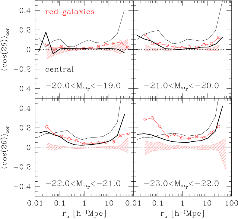
To facilitate the comparison of observed and modeled $\cos(2\theta)$-statistics we follow the observational approach discussed in § 3.3, i.e we use the equivalent luminosity and color cuts. Again the analysis is carried out in projected space where the z-axis is chosen to lie parallel to the line-of-sight and the distant observer approximation is applied. The maximum line-of-sight separation between correlated pairs is restricted to $40{\>h^{-1}\rm Mpc}$. Only the signal based on red ($g-r\geq 0.7$), central galaxies is compared to the corresponding SDSS results. The standard MS reference sample is used.

In Fig. 7 the results for central, red SDSS galaxies are copied from Fig. 3, including the shaded region reflecting the intrinsic scatter in the observational data. The black lines display the corresponding signals derived from the MS. Thick lines represent the results based on central orientations, whereas thin lines are based on halo orientations. In the lowest luminosity bin the halo orientations result in a substantial alignment signal whereas the signal based on the central orientations and the SDSS data are in agreement with no detected alignment signal. For the next two luminosity bins the signal based on central orientations agrees well with the SDSS data. The mismatch for the largest separation bin may be associated with zero-crossing of the correlation function, because the response of the $\cos(2\theta)$-statistic is very sensitive near this point. In the highest luminosity bin there appears a disagreement between the MS signal based on central orientations for separations $\leq 5{\>h^{-1}\rm Mpc}$ and the SDSS measurements. The agreement is better with the MS results based on the halo as a whole. On larger scales $5{\>h^{-1}\rm Mpc}\lesssim r_{p}\lesssim 60{\>h^{-1}\rm Mpc}$ again there is good agreement with the signal based on central orientations whereas that based on overall halo orientations is an overestimate by 50-100 per cent.

We are led to the following conclusions: 1) the alignment signal depends on the magnitude of the central galaxy and/or the mass of the host halo. 2) The alignment signal based on the orientation of the halo exceeds the observed signal, in most cases, whereas the central orientations generally result in good agreement between observations and simulations. 3) The alignment for red central galaxies with $M_{{}^{0.1}r}<-20$ persists to the largest scales probed ($\sim 60{\>h^{-1}\rm Mpc}$).

5 Summary

In the first part of this study we use the SDSS DR6 galaxy catalog to quantify the alignment between galaxies and the large-scale structure. We develop two new statistics, namely the alignment correlation function and the $\cos(2\theta)$-statistic. The former is a two-dimensional extension of the traditional two-point correlation function taking into account the orientations of the main galaxies. The latter is related to the ellipticity correlation function used to analyze cosmic shear observations. In both cases we represent the large-scale structure by a reference galaxy sample with absolute $r$-band magnitudes between $-17$ and $-23$.

The alignment correlation function is defined on the 2D plane of the sky. In our SDSS analysis we use a polar coordinate system and probe the correlation function along the galaxy major axes focusing on the $0^{\circ}<\theta_{p}<30^{\circ}$ sector, where $\theta_{p}$ is the angle between the major axis and the connecting line to a reference galaxy. The abundance of reference galaxies perpendicular to the major axes is represented by the counts within the $60^{\circ}<\theta_{p}<90^{\circ}$ sector. The main results revealed by the alignment correlation function are: 1) The major axes of red galaxies with $M_{{}^{0.1}r}<-20$ are significantly aligned with large-scale structure; 2) The signal is visible out to $60{\>h^{-1}\rm Mpc}$ (the range probed here); 3) Independent of luminosity blue galaxies are not aligned with large-scale structure.

The $\cos(2\theta)$-statistic also probes the anisotropy of the reference galaxies around main galaxies and is related to the galaxy — intrinsic shear correlation function as discussed in Mandelbaum et al. (2006) and Hirata et al. (2007). In contrast to the alignment correlation function it does not require angular binning. It also reveals significant alignment between red luminous galaxies and large-scale structure out to $60{\>h^{-1}\rm Mpc}$ but no alignment is detected for blue galaxies. The restriction to central galaxies results in a slight enhancement of the alignment signal for red galaxies, in particular, at lower luminosities and at large separations. However, the differences are small, indicating little reduction of the signal by satellite galaxies which may have orientations altered by the local tidal field (cf. Pereira & Kuhn 2005).

The second part of this study is based on a Millennium Simulation semi-analytic galaxy catalog where we have assigned an orientation to each red, luminous and central galaxy based on the orientation of the mass distribution of the inner halo. As an alternative identification of the orientation of the central galaxy we also used the orientation of the host halo itself.

The mean projected misalignment angle between a halo as a whole and its central (galaxy) region is $\sim 25^{\circ}$. This misalignment decreases slightly with increasing luminosity of the central galaxy and/or its host halo mass. This behavior is particularly notable, since the relative size of the central region (used to determine the central orientation) decreases with halo mass (cf., Eq. 9).

Based on the orientations and the luminosities of the semi-analytic red galaxies we compute the alignment correlation function in the same manner as for the SDSS galaxy catalog. We find that the alignment signal based on the halo orientations overestimates that found for SDSS. With the central orientation, however, quite good agreement between the modeled galaxy sample and the observations has been achieved. In other words, a misalignment between halo and central orientations is crucial to matching the observed amplitude of the alignment signal. Our approach to compute the major axis of the central elliptical galaxy based on the central dark matter distribution is physically motivated and results in the right amount of misalignment. However, any other process which leads to equal misalignment will be in agreement with our measurements as well.

The large data volume of the MS allows us to generate a two-dimensional map of the alignment correlation function $w_{p}(x,y)$, i.e. we can adopt a very fine two dimensional binning and still get a reasonable number of pair-counts for each bin. The maps based on halo orientation show a substantially flattened galaxy distribution around red main galaxies out to at least $60{\>h^{-1}\rm Mpc}$. Using central orientations the flattening is reduced. In particular we have shown a map based on red main galaxies with $r$-band magnitudes between $-22$ and $-21$ using the standard reference sample. There the ratios of the minor to major axes at $\log w_{p}(x,y)=1.5$, $1$ and $0.5$ are 0.57, 0.61 and 0.42 for halo orientations and 0.75, 0.80, 0.75 for central orientations. It is interesting that the flattening is almost independent of scale all the way from $1{\>h^{-1}\rm Mpc}$ to $60{\>h^{-1}\rm Mpc}$.