Superstatistical generalisations of Wishart-Laguerre ensembles of random matrices

Abstract

Using Beck and Cohen’s superstatistics, we introduce in a systematic way a family of generalised Wishart-Laguerre ensembles of random matrices with Dyson index $\beta$ = 1,2, and 4. The entries of the data matrix are Gaussian random variables whose variances $\eta$ fluctuate from one sample to another according to a certain probability density $f(\eta)$ and a single deformation parameter $\gamma$. Three superstatistical classes for $f(\eta)$ are usually considered: $\chi^{2}$-, inverse $\chi^{2}$- and log-normal-distributions. While the first class, already considered by two of the authors, leads to a power-law decay of the spectral density, we here introduce and solve exactly a superposition of Wishart-Laguerre ensembles with inverse $\chi^{2}$-distribution. The corresponding macroscopic spectral density is given by a $\gamma$-deformation of the semi-circle and Marčenko-Pastur laws, on a non-compact support with exponential tails. After discussing in detail the validity of Wigner’s surmise in the Wishart-Laguerre class, we introduce a generalised $\gamma$-dependent surmise with stretched-exponential tails, which well approximates the individual level spacing distribution in the bulk. The analytical results are in excellent agreement with numerical simulations. To illustrate our findings we compare the $\chi^{2}$- and inverse $\chi^{2}$-class to empirical data from financial covariance matrices.

1 Introduction

Random matrix theory (RMT) is known to find applications in many physical systems [1, 2]. Its central assumption is that the Hamiltonian of the system under consideration can be replaced by an ensemble of random matrices that are consistent with its global symmetries. The matrix elements of such a random Hamiltonian are typically independent Gaussian variables with mean zero and variance one in the real, complex or quaternion domain. These are respectively labelled by the Dyson index $\beta$ = 1, 2 and 4, which in turn corresponds to the invariance group of the ensemble (orthogonal, unitary or symplectic). Another set of ensembles of random matrices, which is well studied in RMT is known as Wishart-Laguerre or chiral ensemble and will be denoted by WL in the following. The WL ensemble contains random matrices of the form [3] $\mathbf{W=X^{\dagger}X}$, where $\mathbf{X}$ is a rectangular matrix of size $M\times N~{}$($M>N$), whose entries are independent Gaussian variables in the simplest case, and $\mathbf{X^{\dagger}}$ is the Hermitian conjugate of $\mathbf{X}$. As such, the WL ensemble contains (positive definite) covariance matrices $\mathbf{W}$ of maximally random data sets. They have since appeared in many different contexts ranging from mathematical statistics, statistical physics and quantitative finance to gauge theories, quantum gravity and telecommunications [4].

The Gaussian distribution of matrix elements above can be obtained by maximising the Boltzmann-Gibbs-Shannon entropy subject to the constraint of normalisation and of fixed expectation value of Tr$\left(\mathbf{X}^{\dagger}\mathbf{X}\right)$ [5]. This observation has been taken by several authors [6] as a starting point for generalising the classical Wigner-Dyson (WD) ensembles, by maximising Tsallis’ non-extensive entropy subject to the same constraints. The resulting distributions of matrix elements are no longer Gaussian but rather follow a power law (for a different generating mechanism of such ensembles see [7]). Recently, a similar generalisation of the WL ensembles has been worked out [8], following earlier studies [9] on the covariance matrices of financial data.

In this context, it is known [10] that the spectral density of covariance matrices built from empirical data may deviate significantly from their purely random (WL) counterpart: in order to obtain a better agreement, it is necessary to introduce correlations among the matrix elements of $\mathbf{X}$, typically allowing the variance of each entry to fluctuate. In [10] this is done using a multivariate Student distribution, where the random entries of $\mathbf{X}$ are written as a product of two variables with a Gaussian and inverse $\chi^{2}$-distribution respectively. Generically, this approach spoils the complete solvability of the model and prevents from going beyond the average spectral density [10]. In order to study other correlations, it is therefore of great interest to introduce generalisations of WL where the independence of $\mathbf{X}$-entries is dropped, but the exact solvability is retained. One of the first examples of such models was provided in [8], where a good fit to the power-law decay of financial covariance spectra was obtained.

It is desirable to place the model [8] within a more general framework, as was done previously for the WD class [11, 12]. The key observation is to resort to the ideas of superstatistics (or statistics of a statistics) proposed by Beck and Cohen [13]. Outside RMT, this formalism has been elaborated and applied successfully to a wide variety of physical problems, e.g., in [14]. In thermostatics, superstatistics arises as a weighted average of ordinary Boltzmann statistics due to fluctuations of one or more intensive parameters (e.g. the inverse temperature). Typically, the distribution of the superstatistical parameter falls into three ’universality’ classes: $\chi^{2}$-, inverse $\chi^{2}$- and log-normal distributions (see section 2.1 for a more detailed discussion). Superstatistical RMT [11] analogously assumes that the Hamiltonian of the system is locally described by a standard WD ensemble with a given variance, and when averaging over the whole system the variance is integrated over with a specific distribution. Consequently, superstatistical RMT is a superposition or integral transform of the usual Gaussian RMTs.

The same concept of integral transforms of standard RMT has also appeared in other contexts, e.g. the fixed or restricted trace ensembles [15], also called norm-dependent ensembles. Very general results can be deduced for them, without specifying the distribution [12, 16]. However, no systematic applications of superstatistics and integral transforms to the WL class are known so far. It is the purpose of this paper to fill this gap.

We are going to introduce first a family of generalised WL ensemble depending on a single real parameter $\gamma$, where the prescriptions of superstatistics are incorporated in a systematic way, and then solve exactly a representative example where the entries of $\mathbf{X}$ are Gaussian random variables whose variances fluctuate from sample-to-sample according to an inverse $\chi^{2}$-distribution. Given the appearance of such a distribution in modelling the volatility of financial markets [10], it is sensible to compute the tail of the spectral density in our model and compare it to the findings in [10] and [8]. However, because of WL ensembles being tailored to times series of data, we expect applications beyond financial covariance matrices as applied here.

Despite the complicated correlations among the entries, and thanks to the integral transform mapping we can go to an eigenvalue basis and write the joint probability density function (jpdf) of eigenvalues as an integral over the corresponding WL one, a feature that was already exploited in [8] for the $\chi^{2}$-distribution. Being able to perform all integrals analytically, we have full control over exchanging the large $N$-limit with our deformation parameter $\gamma$. In the limit $\gamma\to\infty$, our generalised ensembles are designed to recover the standard WL, and this fact will constitute an important consistency check in the following. A third class of models can be obtained by folding with the log-normal distribution, but we will not deal with this case here, lacking a full analytic solution.

It is worth mentioning that the applicability of this formalism is not limited to the above three universality classes. In particular, it would be very interesting to investigate whether the choice of the best superstatistical distribution could be inferred from the data set, instead of being somehow ’postulated’ a priori. This would be reminiscent of the Bayesian approach to superstatistics [17], this time in the more complicated RMT setting.

In the next section 2, we briefly review the prescriptions of superstatistical RMT, together with the three universality classes in subsection 2.1. Then we give a step-by-step derivation of our superstatistical WL ensemble in subsection 2.2. In section 3 we define the spectral properties to be computed in our model and discuss their universality. We then investigate the large matrix size limit of the spectral density in section 4, where we distinguish between square and rectangular matrices of size $N=cM$ in the two subsections. In section 5 we first present a detailed discussion on the applicability of the standard Wigner’s surmise for the level spacing in the WL class, and then we derive a new, generalised $\gamma$-dependent surmise which is appropriate to describe with excellent approximation the individual level spacing in the bulk of our superstatistical model. Numerical checks on the analytical results are provided throughout the text and the algorithm used is described in A. In section 6 we compare two superstatistical distributions to empirical data from financial covariance matrices, before offering concluding remarks in section 7.

2 Superstatistical Wishart-Laguerre ensembles

The probability density of the data-matrix entries in WL ensembles is given by

$$P_{{W\!L}}\left(\eta;\mathbf{X}\right)=\frac{1}{Z_{W\!L}(\eta)}\exp\left[-\eta\beta\Tr(\mathbf{X}^{\dagger}\mathbf{X})\right],$$ (1)

where $\eta$ is proportional to the inverse variance of matrix elements.

The normalisation is given by the partition function

$$Z_{W\!L}(\eta)=\int d\mathbf{X}\exp\left[-\eta\Tr(\mathbf{X}^{\dagger}\mathbf{X})\right]=\frac{1}{\beta NM}\left(\frac{\pi}{\eta\beta}\right)^{\beta MN//2}\ .$$ (2)

As mentioned above, X is a matrix of size $M\times N~{}$ with real, complex or quaternion real elements for the values $\beta$ = 1, 2 or 4, respectively. We parametrise $N=cM$ for later convenience, where $c\leq 1$ distinguishes two different large-$N$ limits. The integration measure $d\mathbf{X}$ is defined by integrating over all independent matrix elements of X with a flat measure. The statistical information about the positive definite eigenvalues of the Wishart matrix $\mathbf{W=X^{\dagger}X}$, or equivalently the singular values of the matrix $\mathbf{X}$ can be obtained integrating out all the undesired variables from the distribution of the matrix elements, using its orthogonal, unitary or symplectic invariance for $\beta=1,2$ and 4 respectively.

We now define a superstatistical family of WL ensembles. The key ingredients are the following:

1. A real deformation parameter $\gamma>0$, which roughly quantifies how far the new model lies from the traditional, unperturbed WL ensemble. In the limit $\gamma\to\infty$, we expect to recover WL exactly.

2. A normalised probability density $f(\eta)$, such that

   $$1=\int_{0}^{\infty}d\eta\,{f}(\eta)\ .$$ (3)

   It is understood that $f(\eta)$ depends on $\gamma$ as well, but we will not show this dependence explicit in order to keep the notation light.

The probability distribution of matrix elements for the generalised model is then obtained as follows:

$$P(\mathbf{X})=\int_{0}^{\infty}d\eta\ f(\eta)P_{W\!L}\left(\ell(\gamma)\eta;\mathbf{X}\right)=\Big{\langle}P_{W\!L}\left(\ell(\gamma)\eta;\mathbf{X}\right)\Big{\rangle}_{f}.$$ (4)

where $\langle\cdot\rangle_{f}$ means average over the distribution $f(\eta)$ and $\ell(\gamma)$ is a simple function of the deformation parameter (see subsection 2.2 below for details). The choice of distribution $f(\eta)$ is determined by the system under consideration. In the absence of fluctuations of the variance, $f(\eta)=\delta(\eta-\eta_{0})$ and we reobtain the standard WL ensemble. Typically, the distribution $f(\eta)$ depends explicitly on the parameter $\gamma$, in such a way that for $\gamma\to\infty$ a delta-function limit is obtained and thus the WL results (before or after taking $N$ large) are duly recovered.

While the distribution defined in eq. (4) is formally normalised, when exchanging the integration $\int d\mathbf{X}$ with $\int d\eta$, the prescription given so far is not complete. The choice of a distribution $f(\eta)$, and in particular of the $N$-dependence of its parameter(s) has to be such that a) the integral over $P(\mathbf{X})$ is convergent, and that b) an $N$ independent limit for the spectral density can be found after a proper rescaling of variables. We will come back to this issue below.

2.1 The three superstatistical classes

Beck et al. [18] have argued that experimental data can be described by one of three superstatistical universal classes, namely the $\chi^{2}$-, inverse $\chi^{2}$-, or log-normal-distribution. Below we briefly discuss each class and the properties of its corresponding distribution, before turning to the detailed solution for the inverse $\chi^{2}$-class in the next sections.

• $\chi^{2}$-distribution:

  The $\chi^{2}$-distribution with degree $\nu$ and average $\eta_{0}$ is given by

  $$f_{1}(\eta)=\frac{1}{\Gamma\left(\frac{\nu}{2}\right)}\left(\frac{\nu}{2\eta_{0}}\right)^{\frac{1}{2}\nu}\eta^{\frac{1}{2}\nu-1}\exp\Big{[}-\nu\eta\frac{1}{2\eta_{0}}\Big{]},$$ (5)

  where we define $\eta_{0}=\int_{0}^{\infty}\eta f(\eta)d\eta\equiv\langle\eta\rangle$. This distribution is appropriate if the variable $\eta$ can be represented as a sum of squares of $\nu$ Gaussian random variables.

  The superstatistical distribution arising from (5) is Tsallis’ statistics with power law tails [19] and is believed to be relevant e.g. for cosmic ray statistics [20].

• inverse $\chi^{2}$-distribution:

  This distribution is found if $\eta^{-1},$ rather than $\eta,$ is the sum of several squared Gaussian random variables. Its distribution $f_{2}(\eta)$ is given by

  $$f_{2}(\eta)=\frac{\eta_{0}}{\Gamma\left(\frac{\nu}{2}\right)}\left(\frac{\nu\eta_{0}}{2}\right)^{\frac{1}{2}\nu}\frac{1}{\eta^{\frac{1}{2}\nu+2}}\exp\Big{[}-\nu\eta_{0}\frac{1}{2\eta}\Big{]},$$ (6)

  with degree $\nu$ and average $\eta_{0}$.

  This class is appropriate for systems exhibiting velocity distribution with exponential tails [21] and was shown to describe the spectral fluctuations of billiards with mixed regular-chaotic dynamics better than the other two distributions [22].

• $\log-$normal distribution:

  In the third class, instead of being the sum of contributions, the random variable $\eta$ may be generated by a multiplicative random processes. Then its logarithm $\log(\eta)=\sum_{i=1}^{\nu}\log(x_{i})$ is a sum of $\nu$ Gaussian random variables $x_{i}$. Thus it is log-normally distributed:

  $$f_{3}(\eta)=\frac{1}{\sqrt{2\pi}\ v\eta}\exp\left[-\left[\log(\eta/\mu)\right]^{2}\frac{1}{2v^{2}}\right].$$ (7)

  It has an average $\langle\eta\rangle=\mu\sqrt{w}$ and variance $\mu^{2}w(w-1)$, where $w=\exp(v^{2})$.

  This class has been found relevant for Lagrangian and Eulerian turbulence [14, 23].

  Because apparently this class does not lead to closed analytical results for the distribution of matrix elements $P_{3}(\mathbf{X})$ or its correlation functions we do not use it as an example in this paper.

2.2 Building the superstatistical ensembles

Since the prescription (4) is not completely straightforward, we provide here a step-by-step construction of the superstatistical probability density $P\left(\mathbf{X}\right)$. We focus here on the inverse $\chi^{2}$-distribution (6) as a new example.

1. We start with the usual WL probability density for the entries, eq. (1):

   $$P\left(\mathbf{X}\right)\rightsquigarrow\exp\left[-\eta\beta\Tr(\mathbf{X}^{\dagger}\mathbf{X})\right]\ .$$ (8)

   Henceforth we omit the normalisation constants.

2. Next, we convolve the WL weight with the inverse $\chi^{2}$-distribution (6):

   $$P\left(\mathbf{X}\right)\rightsquigarrow\frac{1}{\eta^{\frac{1}{2}\nu+2}}\exp\Big{[}-\nu\eta_{0}\frac{1}{2\eta}\Big{]}\exp\left[-\eta\beta\Tr(\mathbf{X}^{\dagger}\mathbf{X})\right]\ .$$ (9)

3. The $\nu$ parameter becomes the deformation parameter of the model as $\gamma=\nu/2$. For a clearer notation, we now make the further replacement $\eta=\nu\eta_{0}\xi/2$ and eventually integrate over the possible values for $\xi$:

   $$P\left(\mathbf{X}\right)\rightsquigarrow\int_{0}^{\infty}d\xi\frac{1}{\xi^{\gamma+2}}\exp\left(-\frac{1}{\xi}\right)\exp\left[-\xi\gamma\beta\Tr(\mathbf{X}^{\dagger}\mathbf{X})\right]\ .$$ (10)

   Note that the average $\eta_{0}$ is no longer needed explicitly and has been absorbed in the other parameters. In (10), the deformation parameter $\gamma$ appears in both the superstatistical weight function and inside the WL Gaussian weight (here $\ell(\gamma)=\gamma$, while in the [8] model $\ell(\gamma)=1/\gamma$).

4. Although formally exact, eq. (10) does not lead to a $N$-independent spectral density, as can be quickly realized with a modest amount of foresight (see (21) and (22)). The last step is thus to amend slightly (10), including a suitable extra factor for normalisation $\xi^{-(\beta/2)NM}$:

   $$P_{2}\left(\mathbf{X}\right)\equiv\int_{0}^{\infty}d\xi\frac{1}{\xi^{\gamma+2-(\beta/2)MN}}\exp\left(-\frac{1}{\xi}\right)\exp\left[-\xi\gamma\beta\Tr(\mathbf{X}^{\dagger}\mathbf{X})\right]\ .$$ (11)

5. Eventually, the integral in (11) can be evaluated, and gives the probability density for the entries of our superstatistical WL model as:

   $$P_{2}\left(\mathbf{X}\right)\propto\Big{(}\Tr(\mathbf{X}^{\dagger}\mathbf{X})\Big{)}^{\frac{1}{2}(\gamma+1-\beta NM/2)}K_{\gamma+1-\beta NM/2}\left(2\sqrt{\beta\gamma\Tr(\mathbf{X}^{\dagger}\mathbf{X})}\right).$$ (12)

   Here $K_{\gamma}(z)$ is the modified $K$-Bessel function of second kind.

This distribution is the main subject of this paper. It is convergent for all values of $\gamma>0$, and we will show later that our choice of the normalisation $\xi^{-(\beta/2)NM}$ effectively leads to an $N$-independent limit for the average spectral density at fixed and finite $\gamma$.

We can analytically recover the standard WL ensemble for $\gamma\to\infty$ (at fixed and finite $N,M$) using the following non-standard asymptotic of the Bessel-$K$ function:

$$z^{\frac{\gamma}{2}}K_{\gamma}(2\sqrt{\gamma z})\sim\sqrt{\frac{\pi}{2}}\gamma^{\frac{1}{2}(\gamma-1)}\rme^{-\gamma}\exp[-z]\ .$$ (13)

While we did not find eq. (13) in tables, it follows easily form the following integral representation 8.432.6 [24], after using a saddle point approximation

$$K_{\gamma}(x)\ =\ \frac{x^{\gamma}}{2^{\gamma+1}}\int_{0}^{\infty}dt\ t^{-\gamma-1}\exp\left[-t-\frac{x^{2}}{4t}\right]\ ,\ \ x^{2}>0\ .$$ (14)

To derive eq. (13) we have included the fluctuations around the saddle point and used the standard notation $f\sim g$ to mean that $f/g\to 1$. The $\gamma$-dependent prefactor can be cancelled by a proper normalisation.

It is important to stress that the choice of the normalisation $\xi^{-(\beta/2)MN}$ does not affect the correct $\gamma\to\infty$ asymptotics in any way, while being the only sensible prescription when taking the large $N,M$ limit at fixed $\gamma$ for the average spectral density (see section 4).

It is also worth mentioning that, following the same steps as above, one can incorporate the other two superstatistical distributions. For example, for the $\chi^{2}$-distribution, one is naturally led to:

$$P_{1}(\mathbf{X}) \propto \int_{0}^{\infty}d\xi\ \xi^{\gamma-1+\frac{1}{2}\beta NM}\rme^{-\xi}\exp\Big{[}-\frac{\xi\beta}{\gamma}\Tr(\mathbf{X}^{\dagger}\mathbf{X})\Big{]}$$ (15)

$$\propto \left(1+\frac{\beta}{\gamma}\Tr(\mathbf{X}^{\dagger}\mathbf{X})\right)^{-\gamma+\frac{1}{2}\beta NM}.$$

The power-law decay of the matrix elements translates into all correlation functions [8], depending on a single rescaled parameter, $\alpha=\gamma-\frac{\beta}{2}NM-1>0$, which is kept fixed in the large-$N$ limit. The reduction back to standard WL can be made both before (and after) the large-$N$ limit using

$$\lim_{\gamma\to\infty}(1+\gamma^{-1}z)^{-\gamma}\ =\ \rme^{-z}\ .$$ (16)

For a more detailed discussion we refer to [8].

3 Generalisation of WL with exponential tails

After introducing the probability distribution of matrix elements in our generalised inverse $\chi^{2}$-WL eq. (11) we go to an eigenvalue basis in this section and define all correlation functions.

The corresponding joint probability distributions function (jpdf) of positive definite eigenvalues $\lambda_{1},...,\lambda_{N}$ of the matrix $\mathbf{W}=\mathbf{X}^{\dagger}\mathbf{X}$ reads

$${\cal P}_{\gamma}(\lambda_{1},...,\lambda_{N})\propto\int_{0}^{\infty}d\xi\,\frac{1}{\xi^{\gamma+2-\frac{\beta}{2}NM}}\exp\Big{[}-\frac{1}{\xi}\Big{]}{\cal P}_{W\!L}(\lambda_{1},...,\lambda_{N};\xi)$$ (17)

$$\propto\prod_{i<j}^{N}|\lambda_{j}-\lambda_{i}|^{\beta}\prod_{k=1}^{N}\lambda_{k}^{\frac{\beta}{2}(M-N+1)-1}\left(\sum_{i=1}^{N}\lambda_{i}\right)^{\frac{1}{2}(\gamma+1-\beta NM/2)}K_{\gamma+1-\beta NM/2}\left(2\sqrt{\beta\gamma\sum_{j=1}^{N}\lambda_{j}}\right).$$

Here we have used the jpdf ${\cal P}_{W\!L}$ of the standard WL ensemble, which is given by

$${\cal P}_{W\!L}(\lambda_{1},...,\lambda_{N};\xi)\propto{\displaystyle\prod\limits_{i<j}^{N}}\left|\lambda_{j}-\lambda_{i}\right|^{\beta}{\displaystyle\prod\limits_{k=1}^{N}}\lambda_{k}^{\frac{\beta}{2}(M-N+1)-1}\rme^{-\xi\gamma\beta\sum_{l=1}^{N}\lambda_{l}}.$$ (18)

For convergence $\gamma$ has to be positive. Both jpdf’s still have to be normalised by the respective partition function $Z_{\gamma}$ and $Z_{W\!L}(\xi)$, obtained by integrating over all eigenvalues.

The $k$-point density correlation functions defined by integrating out $N-k$ arguments of the jpdf are given as:

$$R_{\gamma,\,k}(\lambda_{1},...,\lambda_{k})\equiv\frac{N!}{\left(N-k\right)!}\frac{1}{Z_{\gamma}}\int_{0}^{\infty}d\lambda_{k+1}\cdots\int_{0}^{\infty}d\lambda_{N}{\cal P}_{\gamma}(\lambda_{1},...,\lambda_{N}).$$ (19)

Because of the linear relationship between the jpdf of our ensemble and WL, eq. (17), we can express the $k$-point functions of the former through the latter:

$$R_{\gamma,k}(\lambda_{1},...,\lambda_{k})=\int_{0}^{\infty}d\xi\,\frac{1}{\xi^{\gamma+2-\frac{\beta}{2}NM}}\ \rme^{-\frac{1}{\xi}}\ \frac{Z_{W\!L}(\xi)}{Z_{\gamma}}R_{W\!L,\,k}(\lambda_{1},...,\lambda_{k};\xi),$$ (20)

where $R_{W\!L,\,k}(\lambda_{1},...,\lambda_{k};\xi)$ is the corresponding $k$-point function for the WL ensemble defined in the same fashion. The $\xi$-dependent ratio of the two partition functions which are also linearly related through

$$Z_{\gamma}\ =\ \int_{0}^{\infty}d\xi\,\frac{1}{\xi^{\gamma+2-\frac{\beta}{2}NM}}\ \rme^{-\frac{1}{\xi}}\ Z_{W\!L}(\xi)\ ,$$ (21)

easily follows from eq. (2):

$$\frac{Z_{W\!L}(\xi)}{Z_{\gamma}}\ =\ \frac{\xi^{-\frac{\beta}{2}NM}}{\Gamma(\gamma+1)}\ .$$ (22)

Comparing eq. (22) and (20), it is already apparent that the choice of the normalisation in eq. (10) was in fact necessary to neutralise exactly the $N$- and $M$-dependence coming from the partition functions. In all our formulas, the limit $\gamma\to\infty$ at finite $N$ and $M$ leads back to WL, using eq. (13).

3.1 Universality

We close this section by discussing the universality of generalisations of WL. Following from a variational, generalised entropy principle we should expect a certain robustness of our results, which is indeed the case.

First, all $k$-point correlation functions of the WL ensembles are explicitly known for finite and infinite-$N$, in terms of Laguerre polynomials and their asymptotics. Thanks to the integral mapping eq. (20), the superstatistical models are exactly solvable as well (see e.g. [12, 8]). Also because of this, we could allow for a more general WL ensemble with a polynomial potential $V$ instead of the Gaussian, $\Tr(\mathbf{X}^{\dagger}\mathbf{X})\to\Tr V(\mathbf{X}^{\dagger}\mathbf{X})$, in order to probe the universality of our results under deformations. These non-Gaussian ensembles can again be solved using the technique of (skew-) orthogonal polynomials for any finite $N$ and $M$, and again the complete solvability of the superstatistical generalisation is guaranteed by the very same integral relation eq. (20).

It is known that in the microscopic large-$N$ limit the asymptotic of the orthogonal polynomials for these non-Gaussian models is universal [25, 26] (for rigorous mathematical proofs see [27] and references therein). This implies that the microscopic correlations in our model remain unchanged after the integral transform. As an example for such a microscopic quantity we deal with the level spacing distribution in section 5. For a detailed discussion of the universal microscopic spectral correlations with a $\chi^{2}$-distribution we refer to [8], including references.

About the macroscopic large-$N$ limit, the (generalised) semi-circle and Marčenko-Pastur densities are known to be less robust. They are altered by deformations via a polynomial potential $V$ but still remain computable, see e.g. the discussion in [15] and references therein. However, a different kind of deformation is known that leaves the semi-circle or Marčenko-Pastur density unchanged: the so-called Wigner ensembles (see [28] for a review). The Gaussian random variables of the WL ensemble are replaced by independent random variables with zero mean and fixed second moment. While this generalisation destroys both the invariance as well as the integrability of higher correlation functions, its large-$N$ macroscopic density is the same as in WL, and thus also our integral transform of WL, after taking the large-$N$ limit.

4 The macroscopic spectral density

In this section we focus on the simplest observable, the spectral density $R_{\gamma,k=1}(\lambda)$ obtained by integrating out all eigenvalues but one.

When taking the large-$N,M$ limit, we keep the combination $c=N/M\leq 1$ fixed. This leads to two different behaviours for the WL spectral density: the semi-circle (in squared variables) for $c=1$ and the Marčenko-Pastur (MP) density for $c<1$, see eqs. (24), (4.2) below. Therefore we expect two different limits for our generalised ensembles as well, and the generalisations of these two well-known WL results will be dealt with in two separate subsections below.

Although the average spectral density for WL (and hence for our model as well through eq. (20)) is known explicitly for any finite-$N,M$ in terms of Laguerre polynomials (see e.g. [2, 8]), the generalised spectral density for large $N$ can be obtained following a much simpler route: we replace the finite-$N$ WL quantity under the integral by its large-$N$ result. The correctness of this approach has already been shown in [8]. As a further check, we can eventually take $\gamma\to\infty$ to recover the semi-circle or MP density.

4.1 Generalised semi-circle for law $c$ = 1

In the case $c=1$, the large-$N$ asymptotic expression for the density of eigenvalues of a WL ensembles with distribution $\exp[-\eta\beta\Tr\mathbf{X}^{\dagger}\mathbf{X}]$ eq. (1) is given by

$$\lim_{N\gg 1}R_{W\!L,\,1}(\lambda)=\frac{\eta}{\pi}\sqrt{\frac{2N}{\eta\lambda}-1}\ \ \mbox{with}\ \ \lambda\in(0,2N/\eta]\ ,$$ (23)

and 0 otherwise. An $N$-independent macroscopic density with average one is obtained by rescaling $\lambda\to x\ \langle\lambda\rangle_{W\!L}$ with its mean $\langle\lambda\rangle_{W\!L}=\langle\frac{1}{N}\Tr\mathbf{X}^{\dagger}\mathbf{X}\rangle_{W\!L}=\frac{M}{2\eta}$, calculated with respect to the above distribution. We obtain

$$\rho_{W\!L}(x)\ \equiv\ \lim_{N\to\infty}\frac{1}{N}\langle\lambda\rangle R_{W\!L,\,1}(x\langle\lambda\rangle)\ =\ \frac{1}{2\pi}\sqrt{\frac{4}{x}-1}\ ,\ \ \mbox{with}\ \ x\in(0,4]\ .$$ (24)

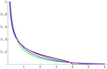
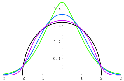
It diverges as $1/\sqrt{x}$ at the origin and vanishes as a square root at the upper edge of support. Eq. (24) corresponds to a semi-circle after mapping eigenvalues from $\mathbb{R}_{+}$ to $\mathbb{R}$, and we will comment more on that below (see Fig. 1).

Following the same procedure as above for the inverse $\chi^{2}$ ensemble, we first need to determine the average eigenvalue in our ensemble (see e.g. [8] appendix A):

$$\langle\lambda\rangle_{\gamma}\ \equiv\ \frac{1}{Z_{\gamma}}\int_{0}^{\infty}d\xi\,\frac{1}{\xi^{\gamma+2-\frac{\beta}{2}NM}}\ \rme^{-\frac{1}{\xi}}\ Z_{W\!L}(\xi)\langle\lambda(\xi)\rangle\ =\ \frac{M(\gamma+1)}{2\gamma}\ ,$$ (25)

using eq. (22) and the mean in WL above.

Next we define the generalised macroscopic $N$-independent density as

$$\rho_{\gamma}(x) \equiv \lim_{N\to\infty}\frac{1}{N}\langle\lambda\rangle_{\gamma}R_{\gamma}(x\langle\lambda\rangle_{\gamma})$$ (26)

$$= \lim_{N\to\infty}\frac{1}{N}\langle\lambda\rangle_{\gamma}\int_{\mathcal{I}}d\xi\ \frac{1}{\xi^{\gamma+2-\frac{\beta}{2}NM}}\ \rme^{-\frac{1}{\xi}}\frac{Z(\xi)}{Z_{\gamma}}\frac{\xi\gamma}{\pi}\ \sqrt{\frac{2N}{\xi\gamma x\langle\lambda\rangle_{\gamma}}-1}\ .$$

Here we have simply inserted the large-$N$ WL density eq. (23) with the parameter $\eta=\xi\gamma$ into the integrand eq. (20). Consequently the interval of integration is truncated and given by $\mathcal{I}=(0,\frac{4}{x(\gamma+1)}]$. Thanks to the correct choice of normalisation in eq. (11), the $N$-dependence completely drops out and for any fixed $\gamma>0$ the new spectral density admits the following integral representation, after changing variables $t=\frac{4}{\xi x(\gamma+1)}-1$:

$$\rho_{\gamma}(x)=\frac{(\gamma+1)^{\gamma+1}}{2\pi\Gamma(\gamma+1)}\ \left(\frac{x}{4}\right)^{\gamma}\int_{0}^{\infty}dt\ \exp\left[-\frac{(\gamma+1)}{4}\,x(t+1)\right]\,(t+1)^{\gamma-1}\ \sqrt{t}\ .$$ (27)

This is our first main result of this section. This density as well as its first moment are correctly normalised to $1$:

$$\int_{0}^{\infty}\rho_{\gamma}(x)dx=1=\int_{0}^{\infty}x\rho_{\gamma}(x)dx\ .$$ (28)

As a consistency check, we can now take the limit $\gamma\to\infty$. The integral becomes amenable to a saddle point approximation, and taking into account the fluctuations around the saddle point we reproduce exactly eq. (24) as we should. Eq. (27) is plotted in Fig. 1 (left) for various values of $\gamma$. Our generalised density has support on the full $\mathbb{R}_{+}$, in contrast with the compact support of the WL semi-circle.

In order to analytically derive the asymptotic behaviour of our generalised semi-circle eq. (27) at the origin $x\to 0$ and at infinity $x\to\infty$ it is more convenient to express the integral through special functions. Using eq. 3.383.5 [24] we can express the density eq. (27) as

$$\rho_{\gamma}(x)=\frac{(\gamma+1)^{\gamma+1}}{4\sqrt{\pi}\Gamma(\gamma+1)}\ \exp\left[-(\gamma+1)\frac{x}{4}\right]\left(\frac{x}{4}\right)^{\gamma}\Psi\left(\frac{3}{2},\gamma+\frac{3}{2};(\gamma+1)\frac{x}{4}\right)\ .$$ (29)

where $\Psi(a,b;z)$ is the Tricomi confluent hypergeometric function (sometimes denoted $U(a,b;z)$). The asymptotics for $x\to 0$ is easy to obtain as:

$$\rho_{\gamma}(x)\sim\frac{(\gamma+1)^{1/2}\Gamma(\gamma+1/2)}{\pi\Gamma(\gamma+1)}\frac{1}{\sqrt{x}}\ .$$ (30)

A few comments are in order. First, the $\gamma$-dependent prefactor in (30) reproduces the correct WL asymptotic behaviour from (24) $\rho_{WL}(x)\sim\frac{1}{\pi\sqrt{x}}$ for $x\to 0$ when $\gamma\to\infty$. Secondly, the WL inverse square root divergence at the origin is not modified in the superstatistical generalisations, a feature that is shared by the $\chi^{2}$-deformed WL [8].

Figure 1: The generalised semi-circle eq. (29) before (left) and after (right) the mapping eq. (33) to $\mathbb{R}$ for different values of $\gamma=0.5,2,10$ (green, blue, violet respectively). For comparison, the standard WL semicircle is plotted as well (black).

Next we turn to the large-$x$ asymptotics. Using only the leading order term [30]

$$\Psi(a,b;z)\ \sim\ z^{-a}\ \ \mbox{for }|z|\to\infty\ ,$$ (31)

we obtain immediately the following result from eq. (29)

$$\rho_{\gamma}(x)\sim\frac{(\gamma+1)^{\gamma-1/2}}{4\sqrt{\pi}\Gamma(\gamma+1)}\exp\left[-(\gamma+1)\frac{x}{4}\right]\left(\frac{x}{4}\right)^{\gamma-\frac{3}{2}}\ .$$ (32)

We illustrate the behaviour of the generalised semi-circle density eq. (29) in Fig. 1. In order to better resolve the behaviour at the origin, we map our spectral density from the positive real axis to the full real axis by defining

$$\vartheta_{\gamma}(y)\ \equiv\ |y|\ \rho_{\gamma}(y^{2})\ ,$$ (33)

that is to a normalised density on $\mathbb{R}$, $\int_{-\infty}^{\infty}dy\vartheta_{\gamma}(y)=1$. Furthermore, this map leads the second moment to be normalised $\int_{-\infty}^{\infty}dyy^{2}\vartheta_{\gamma}(y)=1$. In particular we obtain for WL a semi-circle from eq. (24),

$$\vartheta_{W\!L}(y)=\frac{1}{2\pi}\,\sqrt{4-y^{2}}\ \ \mbox{on}\ [-2,2]\ .$$ (34)

In this squared-variables picture, a further, interesting feature of the generalised spectral density eq. (27) appears when considering the opposing limit $\gamma\to 0$. There, the spectral density admits the following simplified form:

$$\vartheta_{\gamma\to 0}(x)=|x|\frac{\Gamma\left(-\frac{1}{2},\frac{x^{2}}{4}\right)}{4\sqrt{\pi}}$$ (35)

(where $\Gamma(x,y)$ is an incomplete Gamma function), which displays a cusp at $x=0$. This feature often appears in spectral densities of complex networks [31].

As a final remark in the standard WL (or WD) class the density also has an exponential tail at finite-$N$, $\exp[-Nx^{2}]$. However, in the macroscopic large-$N$ limit it disappears while in our deformed model such a tail persists.

4.2 Generalised Marčenko-Pastur law for $c<1$

In this subsection we deal with the limit in which the matrix X remains rectangular, that is both $M$ and $N$ become large with $N/M=c<1$ fixed. We follow the same steps as in the previous subsection, first recalling the results for WL that need to be incorporated into our model. It is known that in the standard WL ensemble eq. (1), the average density of eigenvalues is given for large-$N$ as follows:

$$\lim_{N\gg 1}R_{W\!L,1}(\lambda)\ =\ \frac{\eta}{\pi\lambda}\sqrt{\left(\lambda-\frac{N}{2\eta}X_{-}\right)\left(\frac{N}{2\eta}X_{+}-\lambda\right)}\ ,\ \ \mbox{with}\ \ \lambda\in\left[\frac{N}{2n}X_{-},\frac{N}{2n}X_{+}\right]\ .$$ (36)

Here we have defined the following bounds for later use

$$X_{\pm}\ \equiv\ (c^{-\frac{1}{2}}\pm 1)^{2}\ ,\ \ \mbox{with}\ \ 0<c<1\ .$$ (37)

In the limit $c\to 1$ we recover from eq. (36) the semi-circle eq. (23) from the last section. An $N$-independent density with mean one is again obtained by rescaling with the mean eigenvalue position $\langle\lambda\rangle_{W\!L}=\frac{M}{2\eta}$, and normalising

$$\rho_{MP}(x) \equiv \lim_{N\to\infty}\frac{1}{N}\langle\lambda\rangle_{W\!L}R_{W\!L,1}(x\langle\lambda\rangle_{W\!L})\ =\ \frac{1}{2\pi cx}\sqrt{(x-cX_{-})(cX_{+}-x)}\ ,$$

$$\ \ \mbox{with}\ \ x\in[cX_{-},cX_{+}]\ .$$

This is called Marčenko-Pastur (MP) law [29]. Taking $c\to 1$ we again recover the $N$-independent semicircle eq. (24).

Turning to our generalised model we now insert the large-$N$ result eq. (36) into eq. (20) and rescale with the mean eq. (25)

$$\rho_{\gamma}(x) \equiv \lim_{N,M\to\infty}\frac{1}{N}\langle\lambda\rangle_{\gamma}R_{\gamma}(x\langle\lambda\rangle_{\gamma})$$

$$= \lim_{N,M\to\infty}\frac{\langle\lambda\rangle_{\gamma}}{N}\int_{\mathcal{I}}d\xi\frac{\rme^{-\frac{1}{\xi}}{Z}(\xi)\xi\gamma}{\xi^{\gamma+2-\frac{\beta}{2}NM}{Z}_{\gamma}\pi x\langle\lambda\rangle_{\gamma}}\sqrt{\left(x\langle\lambda\rangle_{\gamma}-\frac{N}{2\xi\gamma}X_{-}\right)\!\!\left(\frac{N}{2\xi\gamma}X_{+}-x\langle\lambda\rangle_{\gamma}\right)}$$

where $\mathcal{I}\equiv\left[\frac{c}{x(\gamma+1)}X_{-},\frac{c}{x(\gamma+1)}X_{+}\right]$ is the truncated integration range. Inserting the ratio eq. (22) and substituting $\xi\to t=\xi x(\gamma+1)/c$ we arrive at the following

$$\rho_{\gamma}(x)=\frac{x^{\gamma}}{2\pi\Gamma(\gamma+1)}\left(\frac{\gamma+1}{c}\right)^{\gamma+1}\int_{X_{-}}^{X_{+}}\frac{dt}{t^{\gamma+2}}\ \exp\left[-\frac{x(\gamma+1)}{tc}\right]\sqrt{(t-X_{-})(X_{+}-t)}\ ,$$ (40)

the second main result of this section. It is valid for any fixed $\gamma>0$ with $0<c<1$. As a check we can take the limit $\gamma\to\infty$, and a saddle point evaluation including the fluctuations around the point $t_{0}=\frac{x}{c}$ leads back to the MP density eq. (4.2).

Next we turn to the asymptotic analysis for $x\to 0$ and $x\to\infty$. For small values of $x$ we simply obtain

$$\rho_{\gamma}(x)\sim D_{\gamma}x^{\gamma}$$ (41)

where the constant $D_{\gamma}$ easily follows from eq. (40). For $x\to\infty$, we obtain:

$$\rho_{\gamma}(x)\sim\frac{\sqrt{X_{+}-X_{-}}}{4\sqrt{\pi}\Gamma(\gamma+1)(X_{+})^{\gamma-1}}\left(\frac{\gamma+1}{c}\right)^{\gamma-1/2}x^{\gamma-3/2}\rm{e}^{-\frac{(\gamma+1)}{cX_{+}}x}\ .$$ (42)

As a check, we can recover the correct asymptotical behaviour (32) when $c\to 1$ (in this case $X_{-}\to 0$ and $X_{+}\to 4$). Note that the decay for large arguments is the same as for the generalised semi-circle eq. (32), in terms of variables $x/(cX_{+})$. An example for eq. (40) is shown in Fig. 2. Such exponentially decaying correlations occur in exponentially growing complex networks, apart from more frequent power law decays [31].

Figure 2: The generalised MP density eq. (40) for $c=0.4$ and different values of $\gamma=0.5,2,10$ (green, blue, violet respectively). For comparison, the standard MP distribution eq. (4.2) is plotted as well (black).

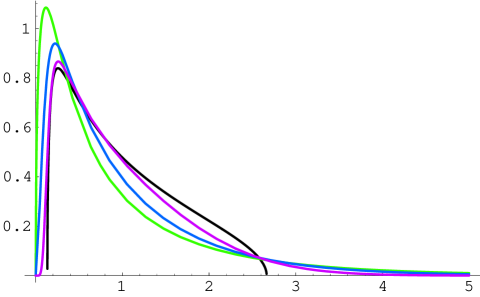
In addition to our analytical checks comparing to WL and $c=1$ we have also performed numerical simulations, generating matrices in our generalised class with the algorithm given in A. In Fig. 3 we compare the numerical results for the spectral density at finite $N,M$ with the theoretical prediction (valid at infinite $N$) eq. (40). We find an excellent agreement already for moderate $N$ and $M$ ($N=10$, $M=40$).

Figure 3: Numerical check for $\beta=1$: Histogram of eigenvalues for $N=10$, $M=40$ and $\gamma=1,10$ (blue and magenta, respectively), together with the theoretical result eq. (40) for $N=\infty$ (black and red solid lines). The average is obtained over $R=50000$ samples.

5 Level Spacing from a Wigner Surmise

The exact computation of the level spacing distribution for finite matrix size $N$ (and in the microscopic large-$N$ limit in the bulk) is mathematically quite nontrivial, even in the simplest case of the WD ensembles, see e.g. [2].

Therefore long ago Wigner came up with the idea to compute the exact spacing distribution in the WD class for the simple $2\times 2$ case, obtaining

$$\mathrm{P}_{W\!D}^{(\beta)}(s)=a_{\beta}s^{\beta}\exp[-b_{\beta}s^{2}]\ .$$ (43)

The $\beta$-dependent constants $a_{\beta},b_{\beta}$ easily follow by fixing the norm and first moment to unity (see e.g. in [1]). Below we will mostly need $\beta=1$ with $a_{1}=\pi/2$, and $b_{1}=\pi/4$. The result eq. (43) turns out to be an excellent approximation of the true result for moderately large $N$, see e.g. Fig. 1.5 in [2], and we aim at a similar approximate representation for the spacing distributions in superstatistical ensembles.

However, before undertaking this more complicated task, we ask the simpler question: does a Wigner surmise using $N=2$ work well in the unperturbed WL ensemble? We have not seen this issue discussed in depth in the literature (see however [32] section V and references therein) and we feel it is appropriate to spend a few words on it in the next section.

5.1 A Wigner surmise in WL?

Starting from eq. (18) for $N=2$ with weight $\exp[-n\beta\lambda]$ ($n=1/2$ for standard normal entries), we can compute the exact spacing distribution ${\cal P}_{\bar{\nu}}(s)$ in WL by integrating over both eigenvalues with the constraint $\delta(\lambda_{2}-\lambda_{1}-s)$. Since this was already done in [8] we can just quote the result:

$${\cal P}^{(\beta)}_{\bar{\nu}}(s)=Cs^{\beta+\bar{\nu}+1/2}K_{1/2+\bar{\nu}}(n\beta s)\ ,$$ (44)

where $K_{\mu}(x)$ is a modified Bessel function, $\bar{\nu}\equiv\frac{\beta}{2}(M-N+1)-1=\frac{\beta}{2}(M-1)-1$, and the constant $C$ is given by:

$$C=\left(2^{-1/2+\beta+\bar{\nu}}(n\beta)^{-3/2-\beta-\bar{\nu}}\Gamma\left(\frac{1+\beta}{2}\right)\Gamma\left(1+\bar{\nu}+\frac{\beta}{2}\right)\right)^{-1}$$ (45)

to ensure a normalisation to unity. The first moment can be normalised by computing

$$d\equiv\int_{0}^{\infty}ds\,s{\cal P}^{(\beta)}_{\bar{\nu}}(s)\ ,$$ (46)

and then defining

$$\hat{{\cal P}}^{(\beta)}_{\bar{\nu}}(s)\equiv d\ {\cal P}^{(\beta)}_{\bar{\nu}}(sd)\ .$$ (47)

The result eq. (47) is obviously different from eq. (43), even for $M=N=2$. Can eq. (47) be a better approximation than eq. (43) for the true WL spacing at $N$ finite but large?

In order to compare, let us pick $N=M$ and $\beta=1$ or $2$ implying $\bar{\nu}=-\frac{1}{2}$ or 0 respectively. The resulting Bessel-$K$ function simplifies only for half-integer index, $K_{1/2}(x)=\sqrt{\pi/2x}\,e^{-x}$, and we obtain

$${\cal P}^{(\beta=1)}_{\bar{\nu}=-\frac{1}{2}}(s) \sim sK_{0}(s)\ ,$$ (48)

$${\cal P}^{(\beta=2)}_{\bar{\nu}=0}(s) \sim s^{2}\exp[-2s]\ .$$ (49)

After normalising the first moment, neither case matches with eq. (43) and for $N\neq M$ (or $\beta=4$) the difference is even more pronounced.

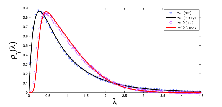
In order to check which spacing distribution is a better approximation for larger $N$ instances, we performed numerical simulations using the Dumitriu-Edelman tridiagonal algorithm [33] for the case $\beta=1$ and $N=M$, with the result shown in Fig. 4. Before commenting on this we mention in passing our procedure. Usually, the numerical quantity to be compared to the surmise is the so-called nearest-neighbour spacing distribution, i.e. the normalized histogram of all the spacings among consecutive eigenvalues in the bulk after unfolding. This procedure is often time-consuming and special care is needed to avoid spurious effects in the analysis (see [32, 34] and references therein for a detailed discussion on unfolding procedures).

We can thus resort to the following, equivalent method to extract the individual spacing at a given location $k$ in the spectrum (see [35]) as:

$$s_{k}\equiv\frac{\lambda_{k}-\lambda_{k-1}}{\langle\lambda_{k}-\lambda_{k-1}\rangle}\ .$$ (50)

The average $\langle\cdot\rangle$ is taken over many samples and obviously $\langle s_{k}\rangle=1$. For a given $N$ we have picked different values of $k$ to check that our results do not depend on the position in the bulk.

Figure 4: Numerical check of the WL and WD surmise for $\beta=1$ and $N=M$: $N=2$ vs. $N=10$ $(13)$, for various locations in the bulk: $k=5,7,8$.

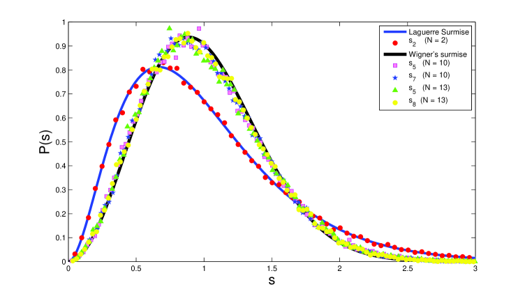
While the numerical histogram for $N=2$ follows the exact result for the spacing from eqs. (48), for increasing $N$ it quickly converges towards the WD surmise eq. (43). We have checked that this holds when choosing $N\neq M$ as well.

What is the explanation? The reason lies in the well known fact that in the bulk both in the WD and WL classes the correlations are governed by the Sine kernel (for a rigorous proof, see [27]). The exact spacing distribution can then be expressed in terms of Fredholm eigenvalues of this kernel, see. e.g. [2], which happens to be well approximated by the WD surmise. This is why the WD surmise applies to both ensembles. In contrast the $N=2$ WL surmise is not a good approximation, and so the surmise does not work here at all. In the next subsection, we seek for a generalised Wigner’s surmise holding in the bulk of our superstatistical model.

5.2 Level spacing for our generalised model

How should an approximate spacing distribution for the generalised WL model with an inverse $\chi^{2}$-distribution be constructed? Because of the failure of an $N=2$ surmise in WL (as we just explained), we should not expect that inserting it into our integral transform will work in the superstatistical case. Instead, we will follow a more heuristic approach confirmed by various numerical checks.

Rather that following the procedure described in subsect. 3.1 we directly start from an integral transform of eq. (43) but with a $\xi$-dependent variance

$$\mathrm{P}_{W\!D}^{(\beta)}(s;\xi)=2\xi^{\beta+1}{\Big{(}\frac{\beta}{2}\Big{)}^{\frac{\beta+1}{2}}}{\Gamma\Big{(}\frac{\beta+1}{2}\Big{)}^{-1}}s^{\beta}\exp[-\beta\,\xi^{2}s^{2}/2]\ .$$ (51)

Eq. (51) is normalised to one (the first moment will be normalised below). Because of $\int d\xi f(\xi)=1$ the following folded surmise for our generalised WL is also normalised:

$$P_{\gamma}^{(\beta)}(s)\equiv\int_{0}^{\infty}d\xi\xi^{-\gamma-2}e^{-\frac{1}{\xi}}\mathrm{P}_{W\!D}^{(\beta)}(s;\xi)=C_{\gamma}s^{\beta}\int_{0}^{\infty}d\xi\xi^{-\gamma-1+\beta}\exp\Big{[}-\frac{1}{\xi}-\frac{1}{2}\beta\,\xi^{2}s^{2}\Big{]}\ ,$$ (52)

with

$$C_{\gamma}=2{\Big{(}\frac{\beta}{2}\Big{)}^{\frac{\beta+1}{2}}}{\Gamma\Big{(}\gamma+1\Big{)}^{-1}\Gamma\Big{(}\frac{\beta+1}{2}\Big{)}^{-1}}.$$ (53)

Figure 5: Level spacing distribution eq. (55) at $\beta=1,2,4$ (from left to right) and different values of $\gamma=1,10,50$ (red, blue, violet respectively). We have also included the WD surmise eq. (43) in green for comparison.

To normalise the first moment we compute

$$d_{\gamma}\equiv\int_{0}^{\infty}ds\,sP_{\gamma}^{(\beta)}(s)=\frac{(\gamma+1)\Gamma\Big{(}\frac{\beta}{2}+1\Big{)}}{\Big{(}\frac{\beta}{2}\Big{)}^{\frac{1}{2}}\Gamma\Big{(}\frac{\beta+1}{2}\Big{)}}$$ (54)

and obtain the approximate spacing distribution in our generalised WL with an inverse $\chi^{2}$-distribution:

$$\hat{P}_{\gamma}^{(\beta)}(s)\equiv d_{\gamma}P_{\gamma}^{(\beta)}(sd_{\gamma})\ .$$ (55)

Eq. (55) is the main result of this subsection. Given the known universality of the (approximate) eq. (43), our new spacing distribution will also be universal under a large class of deformations as discussed in subsection 3.1. The integral can be evaluated in terms of hypergeometric functions, but we prefer to keep the integral form for simplicity. We have checked explicitly that in the limit $\gamma\to\infty$ we correctly reproduce eq. (43) valid for WL $(N\gg 2)$.

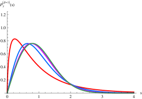
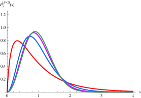
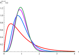
Eq. (55) is plotted for all three values of $\beta=1,2,4$ and various $\gamma$ in Fig. 5, including the limiting WD distribution eq. (43).

Our new surmise eq. (55) has the following asymptotic behaviour. The level repulsion at short distances ${s\to 0}$ is given by

$$\hat{P}_{\gamma}^{(\beta)}(s)\ \sim\ \kappa_{1}s^{\min(\beta,\gamma)}\ ,$$ (56)

At large distances ${s\to\infty}$ however we get a new behaviour in terms of a stretched exponential

$$\hat{P}_{\gamma}^{(\beta)}(s)\ \sim\ \kappa_{2}s^{\frac{1}{3}(\beta+2\gamma-1)}\exp[-\alpha_{\gamma}s^{\frac{2}{3}}]\ ,$$ (57)

which can be obtained after changing variables and making a saddle point approximation ($\alpha_{\gamma}=\frac{3}{2}(\beta d_{\gamma}^{2})^{1/3}$). In both formulae, we have omitted the exact form of the $\gamma$-dependent prefactors $\kappa_{1,2}$.

Figure 6: Comparison to numerical simulations; top: for fixed $\gamma=7$ a comparison between eq. (55) and numerically generated spacings for various combinations of $N,M$ and locations $k$ within the bulk; bottom: for fixed $N=10,\ M=15$ eqs. (55), (43) and numerically generated spacings for various values of $\gamma$ and locations $k$.

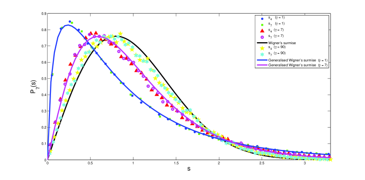
To test our new surmise, we have performed numerical simulations of the individual spacing distribution in the bulk for the most relevant case $\beta=1$ and various values of $\gamma,N$, $M$ and $k$ (the location within the spectrum). Our findings are summarised in Fig. 6, displaying an excellent agreement between the numerical histogram and our surmise.

In Fig. 6 (top), we keep $\gamma$ fixed to the value $\gamma=7$ and vary $N,M$ and the location $k$ within the spectrum. The histogram of the individual $k$th spacing reveals the independence of the spacing on the location $k$ and on $N$ or $M$ (sufficiently greater than $2$). In Fig. 6 (bottom), we keep $N,M$ fixed to the values $(10,15)$ respectively. Increasing $\gamma$ ($\gamma=1,7,90$) we can nicely see the convergence of both the numerical histogram and theoretical curves towards the WD surmise eq. (43).

6 Applications and Discussion

Before comparing to actual data, let us put our results into the context of other models and highlight their features.

From a RMT point of view, the first classification issue is whether or not the considered ensemble is invariant. Preserving invariance leads to a complete solvability for all spectral correlators in our approach as well as in [8]. On the other hand, non-invariant models as in [9, 10, 36] permit generically to compute only the macroscopic density, either implicitly or explicitly. A second issue is that of RMT universality classes, and we argued in section 3.1 that our macroscopic density is universal in a weak sense under (non-invariant) deformations using independent random variables.

A third and important issue is to classify how the spectral density decays for large arguments, even though this may be difficult to appreciate from a small set of data. We have exemplified spectral densities with a power law and exponential decay using a $\chi^{2}$- and inverse $\chi^{2}$-distribution respectively.

About the first issue above, we mention that the non-invariant ensemble [10] using a multivariate student distribution - a product of Gaussian and inverse $\chi^{2}$-distributed random variables - leads to a density with power law decay. Another example is the deformed Gaussian Orthogonal Ensemble (GOE) [36] having an exponential tail as in our more general eq. (32), for the special case of $\gamma=2$ (and $c=1$). This model is non-invariant as well and can be derived from another entropy maximisation procedure [37].

Figure 7: A comparison to 2 sets of spectral densities from financial covariance matrices: top S&P500 price fluctuations of $N=406$ assets of $M=1309$ days between 1991-1996 [40] (see also [38] Fig 1.), and bottom daily price exchanges of the Johannesburg Stock Exchange from Jan 1993-Dec 2002 [39]. In both cases a few higher eigenvalues are omitted. The smooth curves are the spectral densities for the given $c<1$ from a $\chi^{2}$-distribution (green) [8], inverse $\chi^{2}$-distribution (red) eq. (40) and for comparison, the standard MP distribution eq. (4.2) (black).

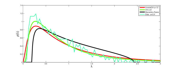
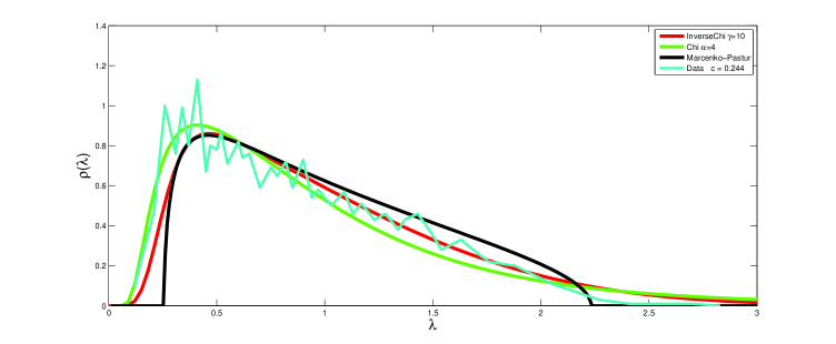
The most natural setting to apply WL or its generalisations is in time series analysis. In Fig. 7 we compare to eigenvalues from financial covariance matrices for 2 different sets of data [38, 39], exploiting superstatistical models with $\chi^{2}$- and inverse $\chi^{2}$-distribution (displaying power law and exponential decay respectively). While in the top plot the former gives a better fit, in the lower plot our new eq. (40) for the inverse $\chi^{2}$-distribution gives at least a comparable if not better fit to the data. We also compare to the standard MP distribution eq. (4.2), which appears to give clearly a less good fit. Because in financial data there is no easy underlying physical principle for identifying extensive variables and thus the distribution class to be applied, our comparison must be heuristic, deciding case by case which distribution gives the best fit.

A similar approach has been taken in a comparison with partly chaotic billiards [22]. Here the microscopic spacing distribution from various generalised WD classes is compared to the data, and the inverse $\chi^{2}$-distribution gives the best fit. Other examples where the inverse $\chi^{2}$-distribution has been recently identified is in turbulent flows [41], although not in a RMT setting.

A very recent example of an application of a superstatistical RMT to complex networks was given in [37]. Here the deformed GOE model [36] within the class of exponentially decaying densities is compared to local statistics of the adjacency matrix. Due to its non-invariance the microscopic RMT predictions there are obtained from simulations. It would be very interesting to calculate these correlation functions analytically in the framework of our model with a more general exponential decay, but this is going beyond the scope of this article.

7 Conclusions

Using the recently proposed methods of superstatistics, we provided a systematic framework for generalising the Wishart-Laguerre ensembles of random covariance matrices, retaining the exact solvability of the original model. This is achieved by allowing the ensemble parameter - the inverse variance of the data matrix elements - to fluctuate from one sample to another according to a certain distribution $f$, and then averaging over $f$. We have given a new compact expression for the distribution of matrix elements in the particular case where the ensemble parameter has an inverse $\chi^{2}$-distribution. This distribution has appeared in the literature when modelling the volatility of financial markets and thus it is of interest for the analysis of large arrays of data. Averaging over this distribution, we are able to express the spectral statistics of the generalised WL ensembles as an integral over the corresponding statistics for the standard WL ensemble. This is the key ingredient to solve the model exactly, for finite-$N$ as well as in both the macroscopic and microscopic limits. In our model we have full control over the interplay between the deformation parameter $\gamma$, the matrix size $N$ and their respective asymptotic limits.

We have computed exactly several spectral quantities, first deriving a generalised semi-circle and generalised Marčenko-Pastur density in the macroscopic large-$N$ limit for square and rectangular data matrices respectively: in both cases, we obtain an exponential tail. Secondly, after discussing in detail the level spacing distribution in WL ensembles and the applicability of the standard Wigner’s surmise, we determined the microscopic level spacing distribution for all three $\beta$ using a new, $\gamma$-dependent surmise, which exhibits a good agreement with numerical simulations.

Our findings are illustrated via an application to financial covariance matrices where we make a comparison between fits resulting from a $\chi^{2}$- and an inverse $\chi^{2}$-distribution. It would be very interesting to find further applications, in particular to time series of other kinds of data.

Acknowledgements: This work started while one of us (A.Y.A-M) was in a short visit to Brunel University. The hospitality of the members of Department of Mathematical Sciences is acknowledged. A.P. Masucci is thanked for providing a reference. Financial support by EPSRC grant EP/D031613/1, European Network ENRAGE MRTN-CT-2004-005616 (G.A.), and European Union Marie Curie Programme NET-ACE (P.V.) is gratefully acknowledged. We are very grateful to R. Kühn for discussions and kindly sharing his data.

Appendix A Numerical Simulations

Since it is not quite trivial to generate matrices with a non-standard Gaussian distribution we briefly describe the algorithm in detail. We focused on matrices with real elements ($\beta=1$) as an example, being the most relevant case for applications.

The algorithm used is the following:

1. Draw a random variable $\xi$ from the inverse-$\chi^{2}$ distribution

   $f(\xi)=\xi^{-\gamma-2}e^{-1/\xi}/\Gamma(\gamma+1)$;

2. Generate a random $M\times N$ matrix $\mathbf{X}$ whose entries are normal variables with vanishing mean, and variance $\sigma^{2}=1/(2\gamma\xi)$;

3. Generate the covariance matrix $\mathbf{\tilde{W}}=\mathbf{X}^{T}\mathbf{X}$;

4. Diagonalise $\mathbf{\tilde{W}}$, obtaining its $N$ positive eigenvalues $\{\mu_{1}^{(\ell)},\ldots,\mu_{N}^{(\ell)}\}$ ($\ell$ stands for the $\ell$th sample);

5. Store:

   - in the matrix row $\mathcal{V}_{\ell,j}$ the rescaled eigenvalues $\{\lambda_{j}^{(\ell)}\}$ ($j=1,\ldots,N$) (where $\lambda_{j}^{(\ell)}=N\mu_{j}^{(\ell)}/\sum_{k=1}^{N}\mu_{k}^{(\ell)}$)

   - in the matrix row $\tilde{\mathcal{S}}_{\ell,j}$ the bare spacings $\tilde{s}_{j}^{(\ell)}=\mu_{j}^{(\ell)}-\mu_{j-1}^{(\ell)}$ ($j=2,\ldots,N$);

6. Iterate the procedure $R$ times, so that $\ell=1,\ldots,R$;

7. Plot i) a normalised histogram of all the entries $\mathcal{V}_{\ell,j}$ (average spectral density) and ii) given a certain $k$ between $2$ and $N$, a normalised histogram of all the entries of $\tilde{\mathcal{S}}$ in column $k$, normalised by the mean $(1/R)\sum_{r=1}^{R}\tilde{\mathcal{S}}_{r,k}$ (individual spacing distribution at location $k$).

The plots of the normalised histograms are then compared with the theoretical results for finite or infinite $N$ respectively (see Figs. 3,4 and 6).

References

- [1] T. Guhr, A. Müller-Groeling, and H. A. Weidenmüller, Phys. Rep. 299, 189 (1998).
- [2] M.L. Mehta, Random Matrices, 3rd ed. (Academic Press, New York, 2004).
- [3] J. Wishart, Biometrika 20, 32 (1928).
- [4] I.M. Johnstone, Ann. Stat. 29, 295 (2001); E. Telatar, Eur. Trans. Telecomm. 10, 585 (1999); E.V. Shuryak and J.J.M. Verbaarschot, Nucl. Phys. A 560, 306 (1993); J.J.M. Verbaarschot, Phys. Rev. Lett. 72, 2531 (1994); J. Ambjørn, C.F. Kristjansen, and Yu. Makeenko, Mod. Phys. Lett. A 7, 3187 (1992); G. Akemann, Nucl. Phys. B 507, 475 (1997); J. Ambjørn, Yu. Makeenko, and C.F. Kristjansen, Phys. Rev. D 50, 5193 (1994); K. Johansson, Comm. Math. Phys. 209, 437 (2000); P. Vivo, S.N. Majumdar, and O. Bohigas, J. Phys. A: Math. Theor. 40, 4317 (2007); S.N. Majumdar, O. Bohigas, and A. Lakshminarayan, J. Stat. Phys. 131, 33 (2008).
- [5] R. Balian, Nuovo Cim. 57, 183 (1958).
- [6] F. Toscano, R.O. Vallejos, and C. Tsallis, Phys. Rev. E 69, 066131 (2004); F.D. Nobre and A.M. C. Souza, Physica A 339, 354 (2004); A.Y. Abul-Magd, Phys. Lett. A 333, 16 (2004); A.C. Bertuola, O. Bohigas, and M.P. Pato, Phys. Rev. E 70, 065102(R) (2004); A.Y. Abul-Magd, Phys. Rev. E 71, 066207 (2005).
- [7] O. Bohigas, J.X. de Carvalho, and M.P. Pato, Phys. Rev. E 77, 011122 (2008).
- [8] G. Akemann and P. Vivo, J. Stat. Mech. P09002 (2008).
- [9] Z. Burda, A.T. Görlich, and B. Wacław, Phys. Rev. E 74, 041129 (2006).
- [10] G. Biroli, J.-P. Bouchaud, and M. Potters, Acta Phys. Pol. B 38, 4009 (2007).
- [11] A.Y. Abul-Magd, Physica A 361, 41 (2006); Phys. Rev. E 72, 066114 (2005).
- [12] K.A. Muttalib and J.R. Klauder, Phys. Rev. E 71, 055101(R) (2005).
- [13] C. Beck and E.G.D. Cohen, Physica A 322, 267 (2003).
- [14] E.G.D. Cohen, Physica D 193, 35 (2004); C. Beck, Physica D 193, 195 (2004); C. Beck, Europhys. Lett. 64, 151 (2003); F. Sattin and L. Salasnich, Phys. Rev. E 65, 035106(R) (2003); F. Sattin, Phys. Rev. E 68, 032102 (2003); A.M. Reynolds, Phys. Rev. Lett. 91, 084503 (2003); M. Ausloos and K. Ivanova, Phys. Rev. E 68, 046122 (2003).
- [15] G. Akemann, G.M. Cicuta, L. Molinari, and G. Vernizzi, Phys. Rev. E 59, 1489 (1999); Phys. Rev. E 60, 5287 (1999).
- [16] T. Guhr, J. Phys. A 39, 12327 (2006).
- [17] F. Sattin, Eur. Phys. J. B 49, 219 (2006).
- [18] C. Beck, E.G.D. Cohen, and H.L. Swinney, Phys. Rev. E 72, 056133 (2005).
- [19] C. Tsallis, J. Stat. Phys. 52, 479 (1988).
- [20] C. Beck, Physica A 331, 173 (2004).
- [21] H. Touchette and C. Beck, Phys. Rev. E 71, 016131 (2005).
- [22] A.Y. Abul-Magd, B. Dietz, T. Friedrich, and A. Richter, Phys. Rev. E 77, 046202 (2008).
- [23] N. Mordant, A.M. Crawford, and E. Bodenschatz, Physica D 193, 245 (2004); S. Jung and H.L. Swinney, Phys. Rev. E 72, 026304 (2005).
- [24] I.S. Gradshteyn and I.M. Ryzhik, Table of Integrals, Series and Products, 6th Edition (Academic Press, London, 2000).
- [25] G. Akemann, P.H. Damgaard, U. Magnea, and S. Nishigaki, Nucl. Phys. B 487, 721 (1997).
- [26] M.K. Sener and J.J.M. Verbaarschot, Phys. Rev. Lett. 81, 248 (1998); B. Klein and J.J.M. Verbaarschot, Nucl. Phys. B 588, 483 (2000).
- [27] A.B.J. Kuijlaars and M. Vanlessen, Commun. Math. Phys. 243, 163 (2003); P. Deift, D. Gioev, T. Kriecherbauer, and M. Vanlessen, J. Stat. Phys. 129, 949 (2007); M. Vanlessen, Constr. Approx. 25, 125 (2007).
- [28] Z.D. Bai, Stat. Sin. 9, 611 (1999).
- [29] V.A. Marčenko and L.A. Pastur, Math. USSR-Sb 1, 457 (1967).
- [30] http://functions.wolfram.com/HypergeometricFunctions/HypergeometricU/06/02/ (2008).
- [31] S.N. Dorogovtsev and J.F.F. Mendes, Evolution of Networks: From Biological Nets to the Internet and WWW (Oxford University Press, Oxford, 2003).
- [32] V. Plerou et al., Phys. Rev. E 65, 066126 (2002).
- [33] I. Dumitriu and A. Edelman, J. Math. Phys. 43, 5830 (2002).
- [34] H. Bruus and J.-C. Anglés d’Auriac, Phys. Rev. B 55, 9142 (1997).
- [35] M. Müller et al., Phys. Rev. E 74, 041119 (2006).
- [36] A.C. Bertuola et al., Phys. Rev. E 71, 036117 (2005).
- [37] J.X. de Carvalho, S. Jalan, and M.S. Hussein, arXiv:0812.5052v1 [cond-mat.dis-nn] (2008).
- [38] Z. Burda and J. Jurkiewicz, Physica A 344, 67 (2004).
- [39] D. Wilcox and T. Gebbie, Int. J. Theor. Appl. Fin. 11, 739 (2008).
- [40] L. Laloux, P. Cizeau, J.-P. Bouchaud, and M. Potters, Phys. Rev. Lett. 83, 1467 (1999).
- [41] E. Van der Straeten and C. Beck, arXiv:0901.2271v1 [physics.data-an] (2009).