,
Power Spectra in a Zero-Range Process on a Ring: Total Occupation Number in a Segment
Abstract
We study the dynamics of density fluctuations in the steady state of a non-equilibrium system, the Zero-Range Process on a ring lattice. Measuring the time series of the total number of particles in a segment of the lattice, we find remarkable structures in the associated power spectra, namely, two distinct components of damped-oscillations. The essential origin of both components is shown in a simple pedagogical model. Using a more sophisticated theory, with an effective drift-diffusion equation governing the stochastic evolution of the local particle density, we provide reasonably good fits to the simulation results. The effects of altering various parameters are explored in detail. Avenues for improving this theory and deeper understanding of the role of particle interactions are indicated.
Keywords: Non-equilibrium processes, Zero-range processes, Driven diffusive systems (Theory)
1 Introduction
For systems in thermal equilibrium, Boltzmann and Gibbs provided a sound framework which forms part of text-book material nowadays. Specifically, the probability distribution (for finding the system in any configuration) is given simply by the Boltzmann factor. In contrast, little is known in general about systems driven into non-equilibrium steady states, specified via, say, a set of transition rates that violate detailed balance. To explore this vast unknown, it is natural to focus on simple solvable models, with the hope of gaining insight for formulating a general framework for non-equilibrium statistical mechanics. One paradigmatic model is the Zero-Range Process (ZRP) [1, 2], in which particles hop from one site to the next on a one-dimensional periodic lattice (i.e., a ring of sites), with a rate that depends solely on , the number of particles in the originating site.
The ZRP distinguishes itself in at least two ways. Its steady-state probability distribution not only takes a factorised form, which can be expressed succinctly in terms of the hopping rate (often easing the computation of various averages). It also exhibits condensation transitions, even in low dimensions which would not be expected in an equilibrium system without long-range interactions. In addition to its utility in the fundamental study of non-equilibrium processes, where it has been employed to develop a general criterion for phase separation in one-dimensional driven systems [3] among other things, the ZRP has also found success as a minimal model for various real systems including vehicular traffic [4], compartmentalised granular gases [5] and gel electrophoresis [6].
Though much is known about the ZRP, there is a simple and natural, but so far unknown, question we may ask. While the total number of particles on the (finite, periodic) lattice is fixed as the system evolves, the number in a subsection of, say, sites – denoted by here – is a quantity that fluctuates in time . In the steady state, its time average is of course a constant. Nevertheless, its average power spectrum, , is non-trivial and provides information on the autocorrelation . A recent study [7] reported the presence of interesting oscillations in the power spectra for another simple paradigmatic non-equilibrium model, the open Totally Asymmetric Simple Exclusion Process (TASEP) [1, 8, 9]. In this work, we carry out an extensive investigation of the ZRP, with a variety of rates and a range of ring and subsection sizes ( and ). In addition to the oscillations discovered in TASEP on an open lattice [7], we found two, “complementary” sets of oscillations, one controlled by and the other, by . If we keep the subsection length fixed and let the ring size go to infinity, we would have the equivalent of an open lattice (with appropriate input and outflux rates to ensure a finite and non-vanishing ). In this sense, our considerations for a closed, periodic lattice can be regarded as inclusive of open lattices as well.
The dynamics of density fluctuations in the ZRP has been investigated recently by Gupta, et. al. [10], who focused on the variance of the integrated current through a single site as a function of time. This quantity also displays damped oscillations, but in the time domain. The period is proportional to , with being the velocity associated with a fluctuation. Being in the frequency domain, our study complements the earlier work. One of the components of our oscillates with period , and undoubtedly can be traced to the same origin. However, in [10], the damping of the oscillations is not the main focus and so, diffusive/dispersive properties in the system were not considered. By contrast, we will analyse such behaviour and find that they pose the most challenge for theoretical understanding. Further, by considering a quantity associated with multiple sites (), we hope to extract more information about the dynamics of fluctuations.
The presence of may lead some to dismiss these phenomena as “nothing but finite size effects.” However, to understand these effects is very important, since many such models of non-equilibrium transport are believed to applicable to physical systems of relatively small s. Thus, in the examples given above, for vehicular traffic and gel electrophoresis. The other popular model of non-equilibrium transport, TASEP, was first introduced as a possible model for protein synthesis [11], where rarely exceeds . By contrast, in traditional macroscopic systems (e.g., in solid state physics), we generally have in mind . Consequently, the phenomena discussed here are not merely of theoretical interest, but should be physically observable.
The paper is organised as follows. Details of the model and its dynamics will be the focus of the next section. Results of simulations, theoretical analysis and comparisons are the themes of the following three sections. We end with a summary and outlook for future research.
2 Model specification and simulation details
The ZRP studied here comprises a one-dimensional lattice of sites with periodic boundary conditions. A total number of particles is placed on the lattice, with no restrictions on the occupation of each site, so that a configuration of the system is completely specified by the set , i.e., particles being on site (with ). This system evolves through particles hopping from site to site. Particles hop to the rightmost adjacent site with a rate that depends only on : . That this hopping rate is independent of the occupation in any other site in the system gives rise to the ZR part of ZRP. A basic diagram of the system is shown in Figure 1.
Ours is perhaps the simplest ZRP, with the particle landing only in the nearest neighbouring site. Many more complex cases exist, e.g., having more than one particle move, landing them in various sites, and inhomogeneous hopping rates: . For a recent review see [2].
Obviously, is a constant in time. The most naive expectation of our simple ZRP is that, after the system settled into a (non-equilibrium) stationary state, the average occupation is homogeneous: . Part of the general interest in the ZRP arises in the existence of a phase transition, when exceeds a critical value , from such a homogeneous state to an inhomogeneous “condensed” state. In the latter, all but one site is occupied by an average of particles, with the excess () in just a single site. Reminiscent of Bose-Einstein condensation, this macroscopic fraction is referred to as the condensate. Unlike the Bose-Einstein case, translational invariance is spontaneously broken and the condensate can reside in any site. Indeed, in a finite system, it does disappear from one site and reappear in another on some interesting time scale [12].
Of the infinitely many functions we can choose for , it is the asymptotic properties that control the existence of a transition. A typical rate is , which allows a condensation transition provided [13]. In this paper, we consider several rate functions, including this one, a constant hop rate, and (which corresponds to having noninteracting particles in the lattice). Despite the interest in condensation and phase transitions, here we will focus on the homogeneous phase of the system, in which many remarkable features already appear. In future studies, we plan to further investigate the power spectra of systems with a condensate, as well as lattices with more interesting topologies [14].
The system is studied using a simple Monte Carlo algorithm. In each Monte-Carlo Step (MCS), we make attempts to move a particle. In an attempt, a site is selected at random. Provided it contains () particles, one is moved to the rightmost adjacent site with probability , where is a normalisation factor, . Of course, a particle leaving site is moved to site . Simulations were typically run for MCS.
Starting from random initial conditions, we discard the first MCS for the system to come to the steady state. Subsequently, we focus on a fixed segment of length sites and record its total occupation,
| (1) |
every MCS. Thus, each of our time series consists of data points, which we regard as samples of points, i.e., with . We choose a power of 2 so that fast Fourier transform routines can be exploited to compute
| (2) |
Finally, we average over the 53 samples to arrive at the power spectrum:
| (3) |
A typical system size of sites was used with varying segment sizes, but most frequently . Mostly, we use the Mersenne Twister [15] random number generator. To rule out systematic errors from these sources, we have also used other generators (e.g., drand48, ran2, /dev/urandom), as well as various data segment sizings and output intervals.
3 Simulation results
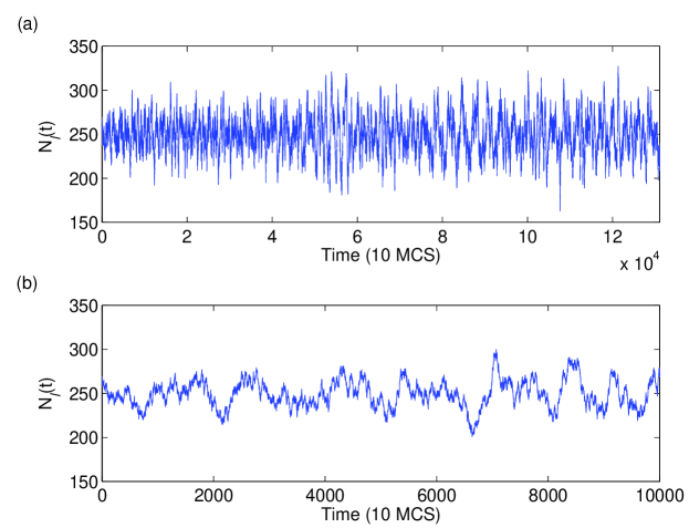
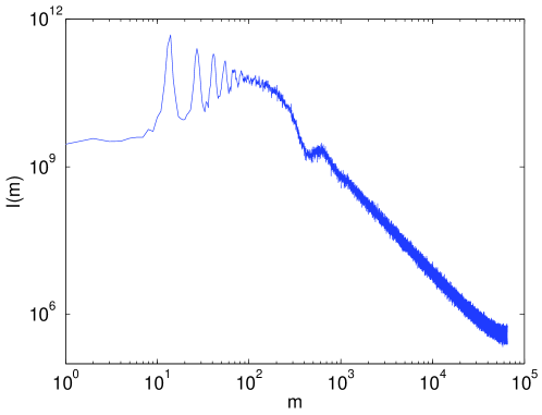
A typical trace of is presented in Figure 2, showing both an entire sample and a magnified view of a section of this sample. It appears that there is some oscillatory behaviour, but it is difficult to distinguish from random fluctuations; taking averaged power-spectra measurements reveals much more in terms of structure. A typical power-spectra measurement is shown in Figure 3 for a system with , and hop rate . It is a log-log plot and the power-spectrum is plotted against the index, , which is related to the frequency, , through the relation . The averaged spectrum displays several prominent features. Two distinct damped-oscillation components can clearly be seen: one at low and the other at higher . The former consists of a series of sharp peaks, with the first peak at . Note the positive curvature at low , a feature notably absent from previously observed power spectra in open systems [7]. The higher- oscillations are more subtle, being obscured partly by the other component. Their character is different, resembling those observed in [7], i.e., “dips” over a smooth background. The first “dip” can be seen at , where the low- oscillations are effectively damped out. For large the spectrum tends to , characteristic of white noise that might be expected for frequencies associated with a microscopic time-scale.
The effects of various parameter variations on the structure shown in the power spectra were studied numerically. These results are discussed in some detail below.
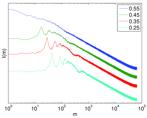
Density — Examining the changes elicited in the power spectrum when varying the density in the system it becomes clear that increasing the overall density lessens and eventually the low- damped oscillating component, Figure 4. However, the same effect is not conclusively observed for the higher- damped oscillations. In fact, simulations at higher values of indicate that this structure remains well into the condensed region, but at high enough density the oscillations will no longer be apparent. It is also notable that the removal of the low- oscillations coincides with the onset of condensation in the system. For the finite systems studied here condensation does not occur with a sharp transition at the theoretical critical density (in this case ) but rather a region of unstable wandering condensates which become more and more stable as the density is increased. In the data shown in Figure 4 there is a moderately-stable wandering condensate for the overall density .
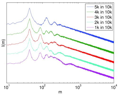
Segment Size — In Figure 5, results are shown for variation in the size of the segment () in the system, keeping the total number of sites () and particles () fixed. Here it can be seen that increasing the size of the segment causes the higher- oscillation component to move to lower and lower where its interference with the other component is increasingly apparent. Thus, it is clear that the structure of the spectrum at high is due to the size of the segment. Note that for a segment of sites in the ring of , the higher- component interferes constructively and destructively with alternating peaks of the low- component.
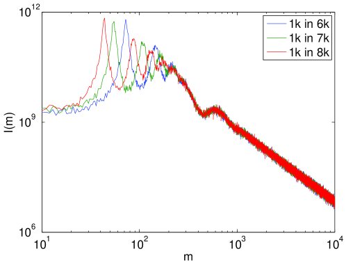
Lattice Size — The effect of changing , the lattice size, was also investigated and results are shown in Figure 6. It is clear that at fixed segment size and particle density, increasing the lattice size changes the low- damped oscillating component but has little effect on the higher- component. In conjunction with the results for segment size, this leads to the conclusion that the higher- component is controlled by the segment size and that the low- component is controlled by the size of the lattice.
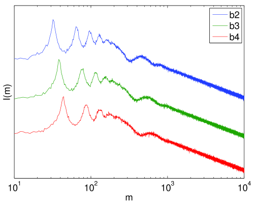
Parameter b — Remaining with the standard hop rate, the effect of varying the parameter (which can be thought of as controlling the strength of the interaction) was investigated. Results for this are shown in Figure 7. It is clear that changing this has an effect on the location of the peaks in both the low- and higher- components. Also, although not immediately apparent from the data presented, it has an effect on the height of the peaks and the number of clearly resolved peaks.
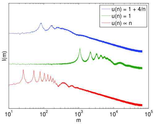
Hop Rate Form — Moving on from the standard hop rate, a comparison of this with constant and non-interacting hop rates is shown in Figure 8. From these results it appears that the two damped oscillation components are most clearly seen in the case of the non-interacting hop rate and least clearly seen in the standard hop rate.
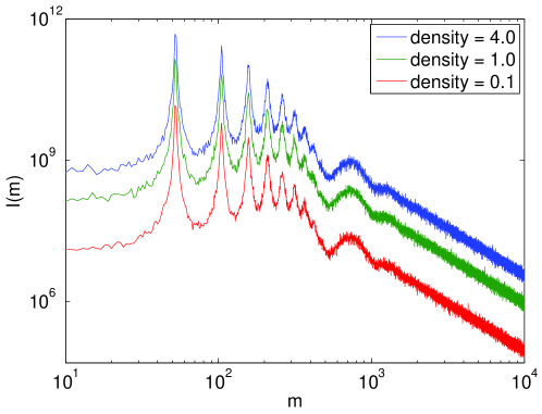
The effect of varying the segment and lattice sizes has much the same effect on the constant hop rate and noninteracting cases as it did with the standard hop rate. However, changing the density continues to affect the power spectra in the case of the constant hop rate, but not for the noninteracting case. In the latter, changing the density merely changes magnitude of the power-spectrum, as shown in Figure 9. This suggests that damped oscillations are universal phenomena in particle-transport systems, though inter-particle interactions will affect the detailed properties. Indeed, we will show in the next section that a drift-diffusion type interpretation is quite successful in describing this phenomenon and that the interaction of the particles controls the values of the drift and the diffusion.
4 Theoretical understanding
Before we present a theory based on the Langevin equation, let us consider a simple toy model, from which we can gain some insight into the origins of both types of oscillations. In this toy model, a single particle moves on a ring of length with uniform velocity , and we seek the power spectrum of , the number of particles in a segment of length . (For simplicity, assume continuous space-time.) Of course, is trivially a series of step functions, such that
| (4) |
where
| (5) |
is the time it takes to traverse the ring and the segment, respectively. Taken over a period of traversals (, to be precise), is given by
| (6) |
Thus,
| (7) |
For sufficiently large, the first of these factors gives a series of “spikes” when is an integer multiple of . Thus, these peaks are controlled by the ring size . By contrast the second factor displays an oscillation over a smooth background (), noticeably with zeros at integer multiples of . We see that these are governed by the segment size . As a toy model, it also serves as a pedagogical tool. What we have here is the temporal version of the diffraction pattern from a large () array of slits of width , spaced a distance apart. Of course, once we add dispersion (velocity here; wavelength in diffraction), we will see both smoothing of the peaks and in-filling of the zeros.
With this insight, we turn to the power spectra here, which can be reasonably well understood through a Langevin equation for the local particle density (continuous variable) on discrete space-time: . To connect with the above section, we may think of as a kind of coarse-grain average of . The starting point is a discrete continuity equation
| (8) |
with being the net local current from site to at time . Clearly, it is controlled by the hop rate . Now, as we are considering power spectra for , we need only account for the deviations of this density from the mean, i.e.,
| (9) |
Except for the condensed phase, is just the global density of particles, ; otherwise, it is (apart from the site with the condensate). The strategy is, for systems far from criticality, these deviations should be small and their essentials can be understood via an approximate Langevin equation that is linear in .
Following the standard route, we recognise the deterministic part of as a function of and expand that to first order in
| (10) |
Defining
| (11) |
and adding the noisy part of the current, , we have
| (12) |
The noise is assumed to be uncorrelated Gaussians, so that
| (13) |
Here, is a measure of the strength of the noise, which we regard as a phenomenological parameter. Before proceeding to the solution, let us emphasise that this somewhat unusual form of the drift-diffusion equation is a signature of the ZRP. In many other driven diffusive systems [16], the current from to would depend on both and , so that an additional term involving will appear on the right hand side of equation (12). By contrast, in the ZRP, the jump rates (from to ) depend only on the occupation at .
In this linear approximation, our Langevin equation (12) can be easily solved by Fourier methods. Defining
| (14) |
where , ( and ), we find the solution easily:
| (15) |
Note that, if we keep terms to lowest (relevant) order in and , the propagator assumes the familiar form,
| (16) |
of a drift-diffusion equation with conserved noise: . For us, the zero-range aspect of the ZRP imposes a relation between and the diffusion “constant” .
Now, our focus here is the number of particles in a segment and so we consider
| (17) |
Carrying out the sum over of , we find (for )
| (18) |
from which we can compute the power spectrum via equation (3). Before comparing such a result to data, we recall that, in the previous study [7], the diffusion coefficient seems to be seriously renormalised by interactions. Anticipating the same behaviour here, we relabel the coefficient of our term (i.e., terms even in ) in the propagator as — the effective diffusion constant — and regard it as a phenomenological parameter. The resulting power spectrum, after performing the average over the noise (equation 13), is
| (19) |
As we will discuss below, to fit the data well, we must choose values of both and to be far from those naively derived above. By contrast, we will see that the “bare” value of (i.e., , with being the known current density relationship of the ZRP [13, 2]) fits the data quite well. At this stage, there is no good explanation for why and are significantly “renormalised,” while seems to be “unscathed.” Our conjecture is that Galilean invariance imposes a Ward identity, as in the case of the driven lattice gas [17]. This is an avenue which we plan to pursue in the future.
Returning our attention to equation (19), we see that it predicts the locations of the first set of peaks (low ones resulting from the sojourn time of a fluctuation around the entire lattice, ) of the power spectra measured from simulation. For example, if we consider small (positive) , we find peaks in whenever vanishes, i.e., ( associated with the terms). In a similar way, introduces oscillations on the scale controlled by the segment length, . In particular, the factor suppresses the peak if is a unit fraction of , i.e., . This behaviour, which is reminiscent of interference, is most pronounced in the case of (top curve ) in Figure 5, where the second peak in the other curves is clearly “missing.” A less prominent “interference” can be seen for the third peak in the middle curve (). If , then such effects will be noticeable only at ’s that are large compared to those among the peaks. In this regime, the damping is so severe that the peaks dissolve into a smooth background and the effects of this factor appear as “dips.”
Turning to the specifics of the ZRP, the current (in the thermodynamic limit) is equal to the fugacity [13, 2], so that will be given by . In the case of the standard hop rate, , the - relation is
| (20) |
so that the velocity is
| (21) |
Similarly, it is easy to show that, in the other cases,
| (22) |
With these analytic results, we are in a position to examine how well this theory fits the simulation data.
5 Comparison between analytic and simulation results
There is generally good agreement between the simple theory presented above and results from simulation, i.e., appropriate choices of the parameters and produce reasonable fits. Not surprisingly, the agreement is best for the noninteracting case. In fact, using as predicted by the theory, the match with simulation results over the entire range of is quite good — see Figure 10. For systems with interacting particles, reasonable fits result only if the effective diffusion constant, , is drastically changed from the naively expected value. Moreover, the quality of the the fit is not uniformly good over all . As an example, in Figure 11, where simulation data (for , , , and , below the condensation threshold) are compared with theory plots with three values of , we see that a value of matches the data reasonably well. To put this result in context, the naive (“bare”) value of the diffusion constant is , so that we would need to invoke “renormalisation effects” at the level of a factor of . Such a sizable “renormalisation” is comparable to that observed in the totally asymmetric simple exclusion process (TASEP) [7]. We believe the origin is universal – inter-particle interactions – and that the resolution of this issue can be applied to both models. Even treating as a phenomenological parameter, the theory fits well only in the midrange, with some discrepancies in the low and high regimes. In the low- regime the peaks and troughs are not ideally fitted by the theory; changing to match this region typically destroys the agreement in the mid-range. For (not shown here), the lack of agreement is also qualitatively similar, with the addition of occasional extra peaks due to a cancellation in the first term in the denominator of 19.
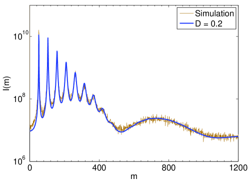
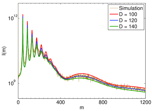
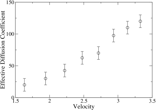
Since is seriously modified by interactions, we investigated systematically the effects of varying various parameters in the ZRP. In contrast, changing the parameters of the non-interacting system leaves the relation completely intact.
Parameter b — The parameter in the hop rate can be thought of as a measure of the strength of the interaction: increasing first makes a condensation transition possible and then reduces , the density at which the transition occurs. With the density, system size, segment size and normalisation () kept constant, the effects of varying are investigated. Now, neither nor varies linearly with , so that we find it more meaningful to plot against (Figure 12), especially to highlight the contrast with for a non-interacting system. From the figure, seems to change with mostly in a linear way, although the intercept of this linear component will not go through the origin. Of course, we should expect more serious non-linear dependence outside the regime shown here.
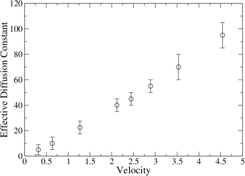
Normalisation — When simulating systems such as the one under consideration here, it is common to assign unit probability to the most likely event, in order to reduce simulation time. This corresponds to choosing . For the data presented in Figure 12 above, this convention was not followed. Instead, a single was used for all the systems (to ensure a conformity of time, ). To explore the effect of varying , we also carried out simulations with the usual convention. The behaviour of with the velocity was found to change dramatically: the previously positive trend of with was reversed. To investigate this further, the effect of changing without other changes was studied. As shown in Figure 13, this gives an apparently linear relationship between and . This is reassuring, since changing alone should correspond to nothing more than changing the time scale, while both and are linear in . More puzzling is the value of the gradient in this plot: The line fits well inside the error bars. Note that a factor of is comparable to the factor shown earlier. We believe that, once the origin of the substantial renormalisation of is uncovered, the resolution of this puzzle will follow.
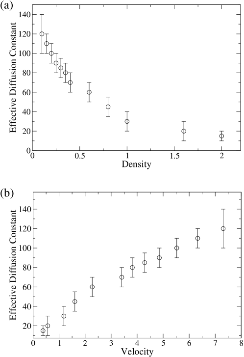
Density — With fixed and , increasing the overall density () lowers both and dramatically. An example of vs. is shown in Figure 14 (a). Once we take into account the - relationship and plot against (Figure 14 b), we again recover the line , with possibly a small negative curvature.
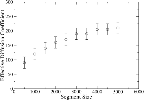
Segment Size — Changing the segment size () has no effect on the velocity, but it does have a pronounced effect on the value of , as shown in Figure 15. The relationship is sub-linear, a behaviour that could be traced to the conserved dynamics. That is, the particle numbers in a segment () plus those in the complementary segment () is a constant, so that the two averaged power spectra must be the same. Unless develops a singularity at the symmetry point, , we must have . From this perspective, a sub-linear variation may have been expected so as to give a flat profile around . However, it is not obvious why the relationship should take this form in general.
System Size — It is also perhaps surprising that varying the system size does not appear to change . It is especially so when taken in conjunction with the fact that changing the segment size does have an effect.
It is best to summarise our findings as follows: Although the observed power spectra can be reasonably well fitted by the predictions of a linear theory, we must regard the effective diffusion constant and the noise amplitude as phenomenological parameters. By contrast, the data is entirely consistent with , the velocity predicted from the theory of ZRPs. It is clear that the simulation results do not support the prediction of the “naive” theory: . In addition, by altering the control parameters in our study (system size, hopping rate, overall density, and segment size), is not only affected dramatically, but also in such a way that its relationship with changes. At this stage, none of these features are well understood.
6 Conclusion
In this paper, we studied the dynamics of fluctuations in the non-equilibrium steady state of the zero-range process (ZRP). Specifically, we collected time series of the number of particles in a contiguous segment of a ring lattice, and computed their average power spectra, . We found interesting structures in , namely, two distinct damped-oscillation components. The small component consists of narrow peaks over a smooth background. The other component resembles broad dips, similar to those observed in the power spectra of open TASEP [7]. The origins of these can be traced to, respectively, the time it takes a fluctuation to travel around the ring and the time for traversing the segment.
We presented a simple toy model, to shed some light on these two types of oscillations: a single particle moving ballistically around a ring in continuous space-time. The time series of the “total particle occupation” in a segment is just a periodic square wave, so that its Fourier transform is the product of a comb and a sinc function, controlled respectively by the ring and segment lengths. Diffusion and noise would broaden the peaks of the comb and fill in the zeros of the sinc function, so that the oscillations will appear damped. Let us emphasise that these oscillations are controlled by the system and segment sizes, so that they are absent from the usual autocorrelation function (for particles at one site, in the thermodynamic limit). Based on the insight from the toy model, we believe these features are universal for the power spectra of all finite driven diffusive systems.
At the quantitative level, the observed can be fitted quite well by a somewhat more sophisticated approach, based on a Langevin equation for the local particle density. Focusing on systems far from criticality, we were motivated to linearise this equation about the average density. The solution of such an approximate equation, even if we account for discrete space-time, is easy. However, except for the case with non-interacting particles, not all the parameters of this simple theory fit the simulation results. In particular, by identifying the even/odd parity (i.e., ) terms with diffusion and drift, we assign the parameters and , respectively. Good fits can be achieved only when is chosen to be considerably larger than the naively predicted value. By contrast, from the simple theory appears to be adequate. At present, we can only present the dependence of on various control parameters as phenomenological results from our extensive simulation studies. In the same vein, the relationship between and (for the range of systems we considered) was seen to deviate significantly from the naive theoretical prediction of . Such “anomalies” associated with were also observed in similar studies of another system [7]. Another puzzling aspect here is that appears to depend more strongly on the segment size () than on the system size (). This feature may indicate that the introduction of an effective diffusion constant to a linear Langevin theory is not an entirely satisfactory treatment. While this approach is somewhat successful at fitting individual power spectra, it leaves much room for improvement, as we seek better understanding and a comprehensive theory.
Although we have ruled out the possibility that these anomalies are due to a systematic effect of our random number generator (by using different generators and choosing parameters to be incommensurate with each other), we have not considered alternative simulation methods. Two such alternatives come readily to mind. One is kinetic Monte Carlo [18], where an appropriate event is chosen at each update and the time advanced according to a Poisson distribution. Another alternative would be to try a common method of reducing simulation times which is to pick a particle at random and hop with an appropriate probability. Fundamentally, we believe that inter-particle interactions are responsible for large deviations from the simple linearised theory presented here, rather than some subtle effect due to the details of the particular dynamics we chose.
It is interesting that similar structures in the power spectra have been observed in two of the most simple models for non-equilibrium systems, namely TASEP and ZRP. Oscillations seen in the variance of the integrated current at a single site in the time domain [10] are also undoubtedly related. These suggest that damped-oscillatory behaviour is universal for finite systems driven out of equilibrium. Further investigations to place this notion on a sound foundation would be worthwhile. It is clear that fluctuations in non-equilibrium steady states are non-trivial and their dynamics induce interesting behaviour. This study has shown only a limited view in a small corner of this vast area. Even within this corner, there is room for improvements, especially in more complete analytic theory. We hope that a better understanding of this particular problem will lead to deeper insights into the nature of fluctuations in physical systems driven far from thermal equilibrium.
References
References
- [1] Spitzer F 1970 Adv. Math. 5 246
- [2] Evans M R and Hanney T 2005 J. Phys. A: Math. Gen. 38 R195
- [3] Kafri Y, Levine E, Mukamel D, Schütz G M and Török J 2002 Phys. Rev. Lett. 89 035702
- [4] Kaupužs J, Mahnke R and Harris R J 2005 Phys. Rev. E 72 056125
- [5] Török J 2005 Physica A 355 374
- [6] van Leeuwen J M J and Kooiman A 1992 Physica A 184 79
- [7] Adams D A, Zia R K P and Schmittmann B 2007 Phys. Rev. Lett. 99 020601
- [8] Schütz G 2001, Exactly solvable models in many-body systems, eds. Domb C and Lebowitz J L, in Phase Transitions and Critical Phenomena Vol. 19 (Academic, London)
- [9] Derrida B 1998 Phys. Rep. 301 65
- [10] Gupta S, Barma M and Majumdar S N 2007 Phys. Rev. E 76 060101(R)
- [11] MacDonald C, Gibbs J, and Pipkin A 1968 Biopolymers 6 1; MacDonald C and Gibbs J 1969 Biopolymers 7 707
- [12] Godrèche C and Luck J M 2005 J. Phys. A: Math. Gen. 38 7215
- [13] Evans MR 2000 Braz. J. Phys. 30 42
- [14] Angel A G, Schmittmann B and Zia R K P 2007 J. Phys. A: Math. Theo. 40 12811
- [15] Matsumoto M and Nishimura T 1998 ACM Trans. on Modeling and Computer Simulation 8 3
- [16] Schmittmann B and Zia R K P 1995 Statistical Mechanics of Driven Diffusive Systems, eds. Domb C and Lebowitz J L, in Phase Transitions and Critical Phenomena Vol. 17 (Academic, London)
- [17] Janssen H K and Schmittmann B 1986 Z. Phys. B64, 503 and Leung, K-t and Cardy J L 1986 J. Stat. Phys. 44, 567 and 45, 1087 (Erratum)
- [18] Young W M and Elcock E W 1966 Proc. of the Phys. Soc. 89 735, Cox D R and Miller H D 1965 The Theory of Stochastic Processes 6, Chatterjee A and Vlachos D G 2007 J. Computer-Aided Mater. Des. 14 253