Dark-energy constraints and correlations with systematics from CFHTLS weak lensing, SNLS supernovae Ia and WMAP5 ††thanks: Based on observations obtained with MegaPrime/MegaCam, a joint project of CFHT and CEA/DAPNIA, at the Canada-France-Hawaii Telescope (CFHT) which is operated by the National Research Council (NRC) of Canada, the Institut National des Sciences de l’Univers of the Centre National de la Recherche Scientifique (CNRS) of France, and the University of Hawaii. This work is based in part on data products produced at Terapix and the Canadian Astronomy Data Centre as part of the Canada-France-Hawaii Telescope Legacy Survey, a collaborative project of NRC and CNRS.
Abstract
Aims. We combine measurements of weak gravitational lensing from the CFHTLS-Wide survey, supernovae Ia from CFHT SNLS and CMB anisotropies from WMAP5 to obtain joint constraints on cosmological parameters, in particular, the dark-energy equation-of-state parameter . We assess the influence of systematics in the data on the results and look for possible correlations with cosmological parameters.
Methods. We implemented an MCMC algorithm to sample the parameter space of a flat CDM model with a dark-energy component of constant . Systematics in the data are parametrised and included in the analysis. We determine the influence of photometric calibration of SNIa data on cosmological results by calculating the response of the distance modulus to photometric zero-point variations. The weak lensing data set is tested for anomalous field-to-field variations and a systematic shape measurement bias for high-redshift galaxies.
Results. Ignoring photometric uncertainties for SNLS biases cosmological parameters by at most 20% of the statistical errors, using supernovae alone; the parameter uncertainties are underestimated by 10%. The weak-lensing field-to-field variance between 1 deg2-MegaCam pointings is 5%-15% higher than predicted from -body simulations. We find no bias in the lensing signal at high redshift, within the framework of a simple model, and marginalising over cosmological parameters. Assuming a systematic underestimation of the lensing signal, the normalisation increases by up to 8%. Combining all three probes we obtain at 68% confidence ( at 95%), including systematic errors. Our results are therefore consistent with the cosmological constant . Systematics in the data increase the error bars by up to 35%; the best-fit values change by less than 0.15.
Key Words.:
Cosmology: observations – Cosmological parameters – Methods: statistical1 Introduction
The Canada-France-Hawaii-Telescope Legacy Survey (CFHTLS111http://www.cfht.hawaii.edu/Science/CFHTLS) has yielded interesting constraints on cosmological parameters using different probes, for example weak gravitational lensing and supernovae of Type Ia. In this paper we combine two recent measurements from the CFHTLS: the cosmic shear data (Fu et al. 2008, hereafter F08) and supernova (SN) Ia data from the Supernova Legacy Survey (SNLS, Astier et al. 2006, hereafter A06). We complement these with CMB measurements from the Wilkinson Microwave Anisotropy Probe (WMAP5, Hinshaw et al. 2009, hereafter H09).
There are hundreds of type-Ia supernovae for which high-quality observations are available. Many surveys spanning wide redshift ranges and using different telescopes and search strategies can be accessed. A recent compilation of various surveys and the derived cosmological constraints can be found in Kowalski et al. (2008). Despite this impressive number of available objects we have chosen to restrict ourselves to the SNLS sample. The resulting constraints will suffer from a greater statistical uncertainty; however, the systematic errors are better understood by using a single, homogeneous survey. By providing imaging with a single telescope and camera for example, SNLS allows a common photometric calibration strategy for the whole survey.
The lensing data presented in F08 might suffer from systematic errors in the shear calibration and shape measurement. In this work, we performed two tests for the presence of systematics. First, we compared the variance between individual MegaCam pointings to simulations. Second, we quantified a potential systematic underestimation of the lensing signal at high redshifts. The influence on cosmological parameters was estimated. Due to the unknown origin of those systematics, the analysis must remain less rigorous than for the SNIa case. It is by no means comprehensive since we only quantify the effect of those systematics and do not investigate their origin, which is beyond the scope of this paper.
The analysis of the five-year WMAP data has yielded impressive results on many cosmological parameters from a great number of models (Dunkley et al. 2009; Hinshaw et al. 2009; Komatsu et al. 2009). Thanks to the rich features in the angular power spectrum, many cosmological parameters can be determined with high precision. However, degeneracies between parameters remain, in particular, for dark-energy models. In order to lift these degeneracies, measurements of CMB anisotropies have to be complemented with other probes.
The WMAP5 team has combined their data with other probes which are sensitive only to the geometry of the Universe, i.e. SNIa and baryonic acoustic oscillations (BAO). Other teams have included probes of structure growth, like counts of X-ray clusters (Mantz et al. 2008), SDSS and Ly-forest (Xia et al. 2008). In this work, we combine WMAP5 with weak gravitational lensing which is sensitive to both the geometry and the growth of structure. Probing both domains will allow future surveys to distinguish between dark energy and modified gravity as a possible cause for the present acceleration of the Universe (e.g. Jain & Zhang 2008). Such a test will be feasible with upcoming and proposed surveys such as KIDS222http://www.astro-wise.org/projects/KIDS, DES333https://www.darkenergysurvey.org, LSST444www.lsst.org, JDEM555http://universe.nasa.gov/program/probes/jdem.html and Euclid666 http://sci.esa.int/science-e/www/area/index.cfm?fareaid=102.
The first-year WMAP data has already been combined with weak lensing, using the RCS survey (Hoekstra et al. 2002), to improve constraints on and (Contaldi et al. 2003). In F08, cosmic shear has been supplemented with the third-year WMAP data. In this work we extend the latter, simple analysis by dropping the (not well motivated) priors on some parameters for lensing ().
The ‘concordance’ flat CDM model of cosmology provides an excellent fit to WMAP5 and most other probes of the geometry and large-scale structure of the Universe. It only contains six free parameters, , , , , and (or functions thereof). This model assumes a cosmological constant as the cause of the observed accelerated expansion of the Universe today. The cosmological constant has yet evaded all plausible physical explanations of its nature and origin and, further, brings in problems of fine-tuning and coincidence. A signature of some ‘dark energy’ beyond a simple cosmological constant might be an equation-of-state (eos) parameter which deviates from the vacuum energy value of . We therefore extend the concordance six-parameter model by including the dark-energy eos parameter . Although this CDM model with a constant is not better motivated physically than the cosmological constant, a significant observed deviation from will definitely be an indication for new physics. Moreover, the data at present are not good enough to constrain more dark energy parameters in a general way. This is only feasible for very specific models, e.g. quintessence (see Schimd et al. 2007) or early dark energy (Bartelmann et al. 2006; Francis et al. 2009), and will be subject of a future work using the CFHTLS data (Tereno et al. in prep.).
One goal of this paper is to focus on systematic errors, nuisance parameters and their interplay with cosmological parameters. For the SNIa data, apart from the usual light-curve parameters, we take into account photometric calibration errors. A joint Bayesian analysis including systematic and cosmological parameters is done and correlations are revealed. This will be mandatory for future surveys with statistical errors which will be smaller by several orders of magnitude as compared to today. To decrease systematics further and further is very challenging, and technical limitations might set a barrier to this endeavour. Therefore, it is important to quantify the effect of systematics and nuisance factors on cosmological constraints.
This paper is organised as follows. Section 2 contains a brief description of the data together with the likelihood used later in the analysis. It also discusses sources of systematics in the data and their correlations with cosmological parameters. In Sect. 3 we define the cosmological model tested in this work, introduce our implementation of the Monte Carlo Markov Chain (MCMC) technique and present the cosmological results of the analysis. We conclude with a discussion in Sect. 4 and an outlook in Sect. 5.
2 Data and method
2.1 CFHTLS-Wide cosmic shear
We use the cosmic shear results from the CFHTLS-Wide year data release (T0003, Fu et al. 2008). On 57 square degrees (35 sq. deg. effective area), about galaxies with -magnitudes between 21.5 and 24.5 were imaged. The data, reduction analyses and shear pipeline are described in detail in F08. We use the aperture-mass dispersion (Schneider et al. 1998) measured between 2 and 230 arc minutes. Due to the compensated nature of its filter, this second-order measure is least sensitive to large-scale systmatics in the data. The source redshift distribution is obtained by using the CFHTLS-Deep (Ilbert et al. 2006) and by rescaling it according to the Wide magnitue distribution and weak-lensing galaxy weights.
To ascertain that the quality and reliability of the shear measurements are sufficient for this work, we perform further tests of the data beyond what has been done in F08. This is addressed in Sects. 2.1.3 and 2.1.2 where we assess the importance of potential systematics for the current data, and estimate their influence on inferred cosmological parameters.
As in F08 the log-likelihood is , where the is modelled as
| (1) |
The predicted aperture-mass dispersion given by a model parameter vector is fitted to measured at angular scales . The covariance of is the one used in F08 and contains shape noise, (non-Gaussian) cosmic variance and the residual B-mode. Those parts of the covariance which depend on the shear correlation (mixed and cosmic variance terms) are calculated using a theoretical model of the large-scale structure and therefore depend on cosmological parameters. We ignore this dependence and keep the covariance constant, corresponding to the fiducial cosmology as in F08. This biases the posterior confidence regions, but the effect is weak over the region of parameter space permitted by CMB and lensing, see Eifler et al. (2008) for a detailed discussion. Moreover, we can drop the term in the log-likelihood because its parameter-dependence manifests itself only for very small survey areas (Kilbinger & Munshi 2006).
As usual, the following relation between the aperture-mass dispersion and the weak lensing power spectrum holds (Schneider et al. 1998),
| (2) |
The lensing power spectrum is a projection of the 3d matter-density power spectrum , weighted by the redshift distribution (Kaiser 1992),
| (3) |
For the non-linear evolution of the power spectrum, the fitting formula of Smith et al. (2003) is used. Although tested for CDM models, it provides reasonable good fits to CDM cosmologies as well (Ma 2007). The accuracy of any non-linear fitting function is limited; when using the ansatz of Peacock & Dodds (1996) instead of Smith et al. (2003), the resulting best-fit differs by 2% (F08).
We parametrise the redshift distribution using the function
| (4) |
which we fit to the obtained redshift histogram. The corresponding is
| (5) |
Here, is the normalised number of galaxies in the redshift bin and the fitting function, evaluated at the redshift bin centre. The uncertainty of contains Poisson noise, photo- uncertainty and cosmic variance, as described in F08 and Benjamin et al. (2007). The sum in eq. (5) extends over the redshift range . In this range, cosmic variance is the dominant uncertainty. As in F08 we neglect the cross-correlation between different bins.
2.1.1 Systematics in the lensing data
In the following two subsections we address the question of potential residual systematics in the cosmic shear data. We estimate the influence of some systematics on cosmological constraints. The shear catalogue used here has been extensively tested in F08. Internal consistency checks have been performed involving the comparison between two data reduction pipelines, residual B-modes and cross-correlations between galaxies and stars. In addition, the shape measurement pipeline has been calibrated with the STEP1 and STEP2 simulations (Heymans et al. 2006; Massey et al. 2007), and a bias of less than 3% has been determined.
Despite that, there are indications of remaining systematics which do not manifest themselves in the merged shear catalogue. For example, there are variations of the shear signal between individual MegaCam pointings which vanish on average. Moreover, with the help of photometric redshifts covering parts of the survey, a problem with the redshift-scaling of the shear correlation becomes apparent.
2.1.2 Variance between CFHTLS pointings
In F08 it was shown the systematics are small globally. The B-mode is consistent with zero on most scales (note however a significant detection around 100 arc minutes). The level of systematics is low on average, e.g. the residual cross-correlation between uncorrected star ellipticities and galaxy shapes after PSF correction. There might however be systematics present on individual fields. Even if they vanish on average they are an additional noise source and increase the measurement error bars.
Here, we address the question whether individual pointings show anomalous variations which might be due to incorrect shape measurements or PSF correction. The field-to-field variance of the lensing signal is compared with numerical simulations.
We measure the shear aperture-mass dispersion on all 57 fields, each one corresponding to a 1 deg2-MegaCam image, and calculate the field-to-field variance. We use -body simulations (Yahagi & Yoshii 2001; Yahagi 2005) through which we shoot light rays to obtain shear maps (Hamana & Mellier 2001) using a redshift distribution corresponding to the mean estimated for the observations. The underlying model is a flat WMAP3-cosmology ().
An important issue are the correlations between CFHTLS-Wide pointings due to large-scale structure. Unfortunately, we cannot simulate the exact survey geometry of the CFHTLS-Wide T0003 survey which extends up to 8 degrees angular separation, since our simulations are only in size. We therefore use several (independent) ray-tracing simulations to cover the observed fields; three for W1, one for W2 and four for W3. This results in less-correlated fields and a smaller cosmic variance compared to the observations. We therefore expect the simulations to slightly underestimate the observed field-to-field variance. The galaxies on each simulated pointing are distributed homogeneously, we do not take into account masking. We do however simulate the varying number density between fields by applying the observed number densities to the simulations.
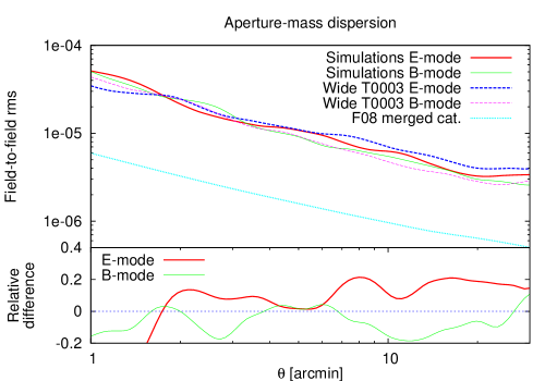
From Fig. 1 we see that the observed E-mode variance of is 10–20% higher than the predicted value, on scales between 1 and 30 arc minutes. The B-mode variance is in very good agreement, with a tendency to be slightly lower than predicted. From the fact that the B-mode variance is of the same order as the E-mode, one sees that the considered angular scales are shape-noise and not cosmic-variance dominated. The power-law shape of the variance is another indication for this. The low-level oscillations on scales on the order of the -correlation length are probably due to noise.
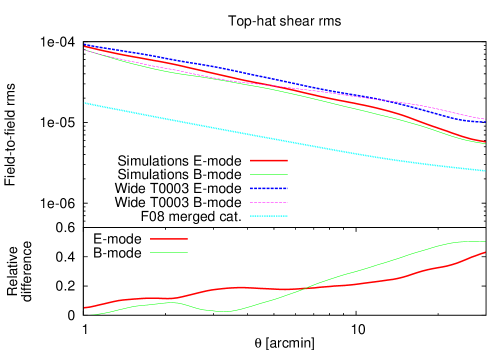
The observed top-hat field-to-field variance is substantially greater than the one from simulations, in particular at large angular scales. This might be due to its higher sensitivity to residuals on large scales compared to the aperture-mass. Note however that because of the high correlations between different angular scales for top-hat, the significance of any discrepancy is hard to interpret. Due to the small number of simulations we cannot attempt an error estimate on the field-to-field variance.
Note that the variance for the merged catalogue used in F08, and this work for the cosmological constraints, is roughly a factor of four less than the one from individual fields.
The greater observed field-to-field fluctuations could be a sign for uncorrected residual systematics. We have not included in the simulations the varying mean redshift due to the different numbers of exposures for each field in the final stacks. The variance in limiting magnitude between fields is 0.25. With the empirical law between limiting magnitude and mean redshift from van Waerbeke et al. (2006) this translates into a -variance of 0.03. Using the approximate relation from linear theory we find an additional expected variance of about 4.5%. We conclude that the observed E-mode field-to-field variance is higher than predicted by at most 5%-15%. It is difficult to assess the influence of this additional error on the complete galaxy catalogue used here. First, we do not know how scales larger than 30 arc minutes are affected. Second, the shear correlation used to constrain cosmology is calculated with many more galaxy pairs than in this field-to-field analysis, with a large number of pairs stemming from different MegaCam pointings.
2.1.3 Systematics in the redshift-scaling of the shear signal
Preliminary analysis of weak lensing tomography of the CFHTLS-Wide shows that beyond a redshift of about unity, the cosmic shear signal does not increase as expected, but instead is systematically underestimated (Fu 2008). For this analysis we use the fourth CFHTLS data release (T0004) which provides five-band photometry on 35 square degrees. Photometric redshifts for each galaxy have been obtained using the template-fitting code Le Phare (Coupon et al. 2009). The quality of the new photo-’s is compatible to those used in F08 (T0003 data release, Ilbert et al. 2006). An improvment has been obtained due to additional and larger spectroscopic samples. We take a sub-set of T0004 consisting of a contiguous area of 19 square degrees. The measured galaxy shapes are the same as in F08.
As an illustration, we show the top-hat shear variance measured at 5 and 25 arc minutes for various redshift bins, see Table 1. The measured values, corresponding to 19 square degrees, are compared to predictions using a flat CDM model with and . For the highest bin with redshifts above 0.95, the measured values are clearly inconsistent with the predictions.
| -range | CFHTLS | Prediction | CFHTLS | Prediction |
|---|---|---|---|---|
| 0.95 | 0.29 | |||
| 2.38 | 0.73 | |||
| 4.12 | 1.27 | |||
| 4.77 | 1.48 | |||
| 7.46 | 2.33 | |||
We have to assume that this anomalous redshift-scaling is also present in the shear catalogue used in this paper for the cosmology constraints. The redshifts for this preliminary analysis are taken from the CFHTLS Wide and are therefore slightly less accurate than the T0003-Deep ones, used to infer the F08 redshift distribution. However, the former do not suffer from cosmic variance. The calibration with spectroscopic redshifts assures their reliability for . The depth of the F08 shear galaxies is only half a magnitude higher, and those faint galaxies are down-weighted in the weak lensing analysis. We therefore assume that the problem is mainly due to the shape measurement and not to the photometric redshifts. One reason for this could be a shear calibration bias which depends on galaxy properties that are a function of redshift. A bias in the shape measurement which is a function of galaxy size, magnitude or galaxy signal-to-noise will affect low- and high-z galaxies differently.
For this work we choose a simple toy model to parametrise this potential underestimation of the redshift-scaling of the shear signal, see Lesgourgues et al. (2007) for a similar approach. This decrease of the lensing signal corresponds to an effective lensing efficiency which is lower than expected at high redshifts. To model this we multiply the redshift distribution with a constant , for redshifts . We chose to be 1.0. is the unbiased case with no degradation of the shear signal. is the pessimistic case where there is no shear signal for . We allow values greater than unity corresponding to an overestimation of the shear signal. Note that we use the original, unaltered redshift distribution when fitting the histogram (eq. 5).
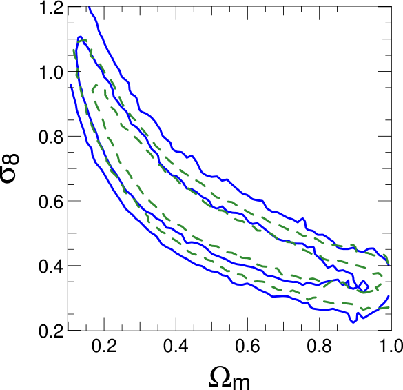
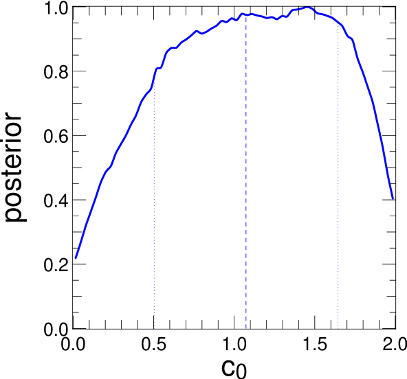
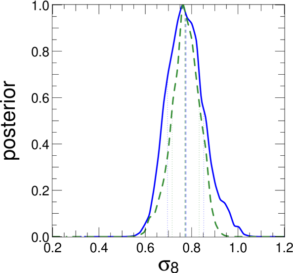
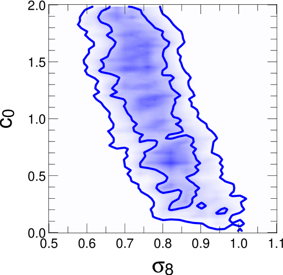
Using a model with fixed and and marginalising over and redshift parameters we measure a value of consistent with unity but with large error margins, (see also Fig. 2, right panel). At 95% confidence nearly the whole range of is permitted. Ignoring the high- calibration error leads to smaller error bars for other parameters, in particular (left panel of Fig. 2). For a fixed we respectively get and with and without modelling the systematic error. Because we allow the calibration to be smaller and greater than unity there is no significant bias on . If we restrict to values smaller or equal 1, thus using the information about the underestimation of the shear signal as prior, we obtain a best-fit of 0.83 (). Thus, might be underestimated by which is about one sigma, provided our simple model is correct. From Fig. 3 (left panel) we see the potential shear measurement systematics shifts the likelihood and introduces a tail for high .
We repeat the above analysis with and 1.2 and find only small shifts for the power-spectrum normalisation. Writing , we find if is varied between 0 and 2, and for , corresponding in both cases to a 2% change for in the considered range for .
Interestingly, we see no correlation between and any other individual parameter when the whole posterior is considered. However, is of course correlated with the combination of and which determines the shear amplitude. When fixing we see a strong correlation with , as expected (Fig. 3, right panel).
To summarise the results on weak lensing systematics, we note that this study is far from complete. Other tests focusing on the PSF correction have been made in F08, and extensive studies going into much more detail as presented here will be published soon (van Waerbeke et al. in prep.).
2.2 SNLS supernovae Ia
The supernova data set corresponds to the first data release of the SNLS, see A06. We use 105 supernovae in total, 71 of which were observed with the CFHTLS. Their redshift range is between 0.25 and 1. The remaining 44 objects are nearby supernovae, with . In the next section (2.2.1) we describe the ingredients of the standard likelihood analysis, ignoring systematics, which is similar to A06 with slight modifications. Section 2.2.2 introduces the photometric calibration parameters and defines the updated likelihood function including systematics.
2.2.1 Standard likelihood analysis
We use the results from the SNIa light-curve fits of A06. For each supernova the fit yields the rest-frame -band magnitude , the shape or stretch parameter , and the colour . These quantities are combined in the estimator of the distance modulus for the object as follows:
| (6) |
The universal absolute SNIa magnitude is ; and are universal linear response factors to stretch and colour, respectively.
The error needed for the likelihood includes: (1) The measured uncertainties of the light-curve parameters and their correlations. The corresponding error contribution to can be written as with the parameter vector and the covariance of the data vector . (2) An additional redshift uncertainty due to peculiar velocities corresponding to km s-1. (3) An intrinsic scatter in absolute magnitude of .
Those three errors are added in quadrature to the log-likelihood expression, which is
| (7) |
The linear dependence on the Hubble constant of the luminosity distance is taken out as an additional summand in eq. (7) and integrated into the absolute luminosity. From now on we will use the parameter .
The error term from the light-curve fit, , depends on the stretch and colour responsitivies and . A06 kept those parameters fixed during the -minimisation and updated them iteratively in consecutive minimisation runs. This leads to a bias in those parameters of 7% - 15%. Instead, we include the dependence of and in the denominator in eq. (7) to obtain unbiased best-fit results for those parameters which are therefore larger than those cited in A06, see Table 4.
We do not take into account the term involving the covariance determinant in the log-likelihood. Even though in this case this term is not a constant because of the parameter-dependent variance, we verified that the effect on cosmological parameters is very small. Moreover, it is in accordance to most other SNIa analyses (e.g. Astier et al. 2006; Kowalski et al. 2008).
2.2.2 Extended analysis with systematics
We extend the analysis of A06 by including the response of the distance modulus to a photometric zero-point shift in each of the seven filters and in the Vega colour in the Landolt system. The reference photometric zero-points are those used in A06, which were estimated without using the Hubble diagram. If denotes the vector of those eight zero-point magnitude shifts, the linear response is the change in distance modulus for the supernova for a small change of the zero-point,
| (8) |
By changing the zero-points and redoing the light-curve fit, we obtain the values of for each supernova. We include this change to the distance modulus linearly in the model, which results in an additional term in the likelihood.
We assume that the zero-point magnitude shift parameters are uncorrelated variables, since the data in different optical bands have been reduced independently. The noise is the result from a number of different source and can therefore be well approximated to be Gaussian. By definition they mean of is zero. The rms is taken to be for all filters except for () where we assume the rms to be . The numerical values of those uncertainties are taken from A06 (Sect. 4.1) and correspond to the limits of reproducibility of the photometric calibration. The corresponding (diagonal) covariance matrix is .
This prior information is multiplied to the SNIa-likelihood in the form of a multi-variate Gaussian likelihood. With the additional term, the log-likelihood expression corresponding to the extended analysis is then
| (9) |
Now, the parameter vector contains the zero-point parameters . The corresponding optical bands are indicated in Table 2.
| Light-curve parameters | ||
|---|---|---|
| Zero-point shifts | ||
2.2.3 Systematics for SNIa
Unlike systematics in weak lensing shape measurements which are difficult to model, the observation-related systematics for SN are more easily parametrised. In the next section we take into account errors in the estimated distance modulus due to uncertainties in the photometric calibration. The results of the MCMC analysis for the SNIa internal parameters are given in Table 4.
2.2.4 Bias due to systematics
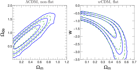
We compare the case of ignoring the systematic errors, using eq. (7) as the log-likelihood, with the case of fully taking into account the systematics according to the log-likelihood (9). As can be seen in Fig. 4, ignoring the zero-point errors leads to an asymmetric decrease of the error bars. The constraints get tighter, mainly along the direction of constant luminosity distance, which is the parameter-degeneracy direction. The error bars decrease by about 10%, see Table 3. The bias on parameter means is small, between 10% and 20% of the statistical uncertainty. The bias on the intrinsic SNIa parameters () is even smaller, not more than a few percent of the statistical uncertainty. For a fixed , the absolute biases on both the eos parameter (for ) and the dark-energy density (for ) are smaller than for the marginalised case, but remain to be about a tenth of the statistical error.
| With systematics | Ignoring systematics | |
| flat Universe | ||
| With systematics | Ignoring systematics | |
As mentioned in Sect. 2.2, we obtain unbiased best-fit values for the stretch and colour response parameters, and , respectively (see Table 4). These differ by about 15% from the (biased) values given in A06. The absolute magnitude is consistent with A06.
The parameters describing the zero-point shifts ( to ) are all consistent with zero (Table 4). Except for they have zero mean and rms of about . The influence of the derivative (eq. 8) on the second term of the likelihood (eq. 9) is small in comparison with the first term. Nevertheless, correlations with other parameters are introduced as is discussed in the next section. The mean of the -band zero-point shifts is negative (although not significantly so) and its variance smaller than the expected value of . It is also this parameter which shows the highest correlation with cosmological parameters.
| Parameter | Best-fit-value |
|---|---|
2.2.5 Correlation between systematic errors and cosmological parameters
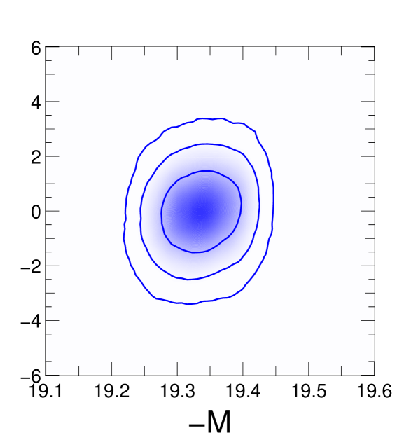
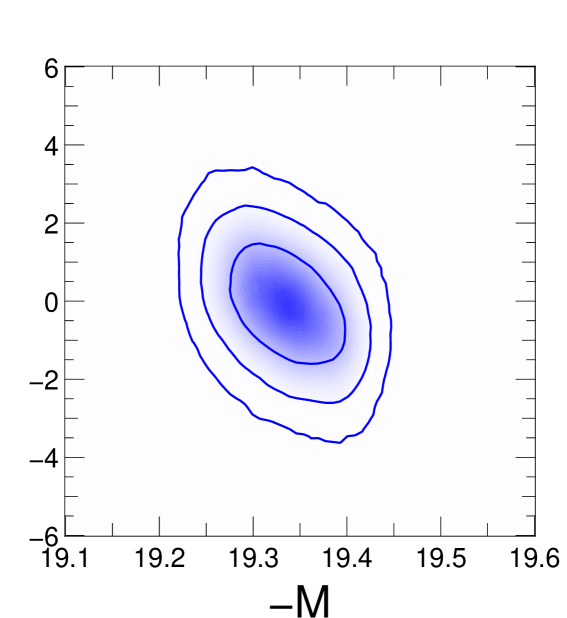
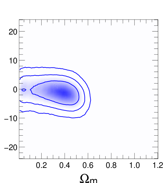
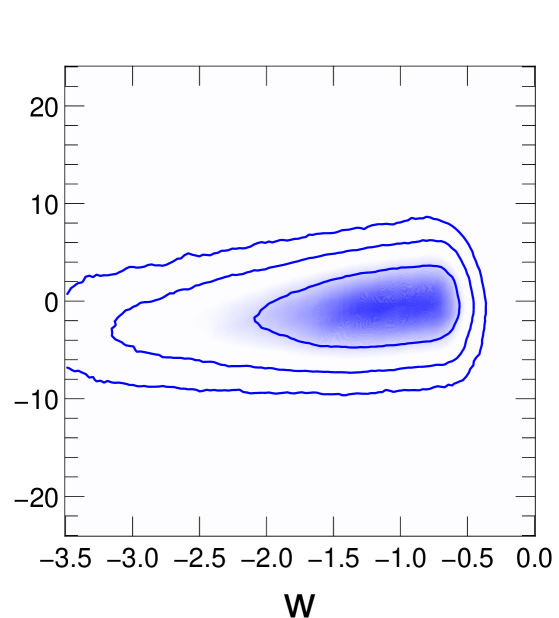
In most cases the zero-point shifts are uncorrelated with other parameters. However, some pairs of one or more nuisance parameters show correlations, most notably, the absolute SNIa magnitude is correlated both with the - and -band uncertainty and , respectively, see Fig. 5. This correlation can be explained by looking at the rest-frame colour parameter, , which contains the colour excess at the time of the -band maximum. Redefining the - or -band zero-points causes a systematic change in which is compensated by a corresponding change in . The slope of the measured -correlation is about 1.5. The correlation between and is much weaker and has a smaller slope of -0.3 to -0.4. The correlation between and the difference is therefore on the order of the best-fit value of , which is expected from eq. 6. The difference in correlation can be explained by the fact that the observed magnitudes of each object translate into different rest-frame bands for the light-curve fit depending on the object’s redshift.
Further, the -band zero-point offset () shows a correlation with both and (Fig. 6). We find and . The latter value can be compared to A06 (Table 5) who varied the zero-points to infer the influence on cosmological parameters; our value is of the same order of magnitude as the one from A06 but has opposite sign. For a fixed we obtain , about half of the value cited in A06 (Table 5).
2.2.6 Further sources of systematics
A06 discussed further sources of systematic uncertainties which can affect cosmological results from SNIa. Some of those uncertainties could be parametrised and invoked in a joint analysis with cosmology as presented in this paper. We state a few more examples here and leave a thorough analysis for future work.
For example, the difference between measured rest-frame -band magnitude and the one ‘predicted’ from the light-curve fit using only two bands can be included in the likelihood function.
In addition, the Malmquist bias can be modelled as a function of redshift. The inclusion of this bias will be necessary when redshift-dependent dark-energy models are to be tested. This requires accurate knowledge of the sample and of selection effects.
2.3 WMAP5 CMB anisotropies
To calculate CMB temperature and polarisation power- and cross-spectra we use the publicly available package CAMB777http://camb.info (Lewis et al. 2000). The likelihood is evaluated using the public WMAP5 code888http://lambda.gsfc.nasa.gov (Dunkley et al. 2009). We include all ‘standard’ components which are the same for three- and five-year. Those are the low- TT and TE/EE/BB spectra, the high- TT and TE spectra, and the point-source TT correction. The low- ( for TT, for polarisation) likelihoods are calculated using Gibbs sampling (Page et al. 2007; Dunkley et al. 2009). The high- sampling uses pseudo- according to Hinshaw et al. (2007).
In contrast to the published WMAP5 results, we do not include corrections due to SZ. The SZ amplitude is unconstrained by WMAP5 and is not degenerate with other parameters (Dunkley et al. 2009). A recent analysis found no biases for WMAP5 when ignoring the contribution of the thermal SZ effect from clusters (Taburet et al. 2009).
3 Parameter analysis and cosmological constraints
3.1 Cosmological model and parameters
We assume a flat dark-energy cold dark matter cosmology (CDM) with the parameter vector . Clustering of dark energy is not taken into account. For CMB, instead of the normalisation defined at a scale of 8 Mpc/h, , the parameter which is sampled is , the curvature perturbations amplitude at the pivot scale . As stated in Sect. 2.1 we use the Smith et al. (2003) fitting formula to model the non-linear power spectrum needed for weak lensing. We do not include a massive neutrino component to the mass-energy tensor and assume as the effective number of massless neutrinos (Mangano et al. 2002), which is the preferred value for WMAP5 (Dunkley et al. 2009). Tereno et al. (2008) obtained constraints on the neutrino mass using various probes including CFHTLS-Wide weak lensing, see also Gong et al. (2008) and Ichiki et al. (2009). Additional parameters are from lensing and from SN Ia. These parameters are described in the respective subsections of Sect. 2; including systematics we sample a total of 22 parameters.
3.2 Sampling the parameter space with MCMC
We use an adaptive Metropolis-Hastings algorithm (Metropolis et al. 1953; Hastings 1970) to generate Monte Carlo Markov Chains (MCMC) as sample of the posterior. The Fisher matrix evaluated at the maximum-likelihood (ML) parameter serves as initial multi-variate Gaussian proposal. The ML point is estimated by a conjugate-gradient search (Press et al. 1992). For lensing and SNIa the typical chain length is 100 000 with an acceptance rate of about 15%-20%. Every 1 000 steps the chain covariance is updated and replaces the previous proposal. The proposal variance is multiplied by a factor which is optimal for a Gaussian posterior (Hanson & Cunningham 1998; Dunkley et al. 2005).
For WMAP5 on the other hand, we choose a different strategy. With acceptance rates as stated above we found the posterior not well sampled and as a consequence the parameter uncertainties largely underestimated. We refrain from updating the proposal but kept the initial guess, which is larger than the Fisher matrix, for the whole duration of the chain. This choice results in small acceptance rates of 3% to 10% but guarantees an unbiased sampling of the posterior.
The experiments are combined by multiplying the corresponding likelihoods or, equivalently, by summing up the log-likelihoods. The confidence intervals are obtained by creating histograms of the parameter vectors of the chain and estimating regions with 68%, 95% and 99.7% of the density.
In particular for WMAP5 the calculation of the converged chain is very time-consuming and takes a few days to a week on a fast multi-core machine. To overcome this and other problems related to MCMC, such as the difficulty to assess convergence and the high correlation of a Markov chain, a new method called Population MonteCarlo (PMC, Cappé et al. 2004, 2007) has been developed which is based on adaptive importance sampling. In a companion paper, we test this method with simulations and apply it to cosmology posteriors (Wraith et al. 2009).
3.3 Combined constraints from lensing and CMB
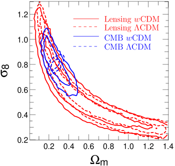
The main contribution from cosmic shear (without tomographic information), in combination with CMB anisotropy measurements, are constraints on the normalisation (Contaldi et al. 2003; Tereno et al. 2005). For a CDM model, the degeneracy direction between and is orthogonal between lensing and CMB. Lensing is sensitive to the amount of structure and therefore, a high normalisation has to be countered by a smaller amount of the total matter. On the other hand, an overall increase of the CMB angular power spectrum by a higher normalisation has to be compensated by more matter to dampen the peaks.
This picture changes if the dark energy equation-of-state is a free parameter. Whereas the lensing contours for and do not broaden much, the CMB constraints increase dramatically. Most importantly, they increase along the lensing-direction of degeneracy, see Fig. 7. The result is that adding lensing to CMB data will not improve the constraints in the - plane as much as it would do in the framework of a cosmological constant model.
Lensing without tomography is not very sensitive to , thus leaving it a free parameter has a minor influence on the other parameters. For CMB however, strong correlations enter through the angular diameter distance which CMB measures only at . Those degeneracies (see Fig. 9) can be broken by adding an additional distance measurement at low redshift as a lever, e.g. using BAO or SNIa, (Frieman et al. 2003; Blake & Glazebrook 2003; Seo & Eisenstein 2003).
3.4 Combined constraints from lensing, SNIa and CMB
| Parameter | CMB | CMB+Lens | CMB+SN | CMB+Lens+SN | CMB+Lens+SN+sys |
|---|---|---|---|---|---|
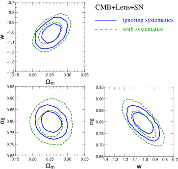
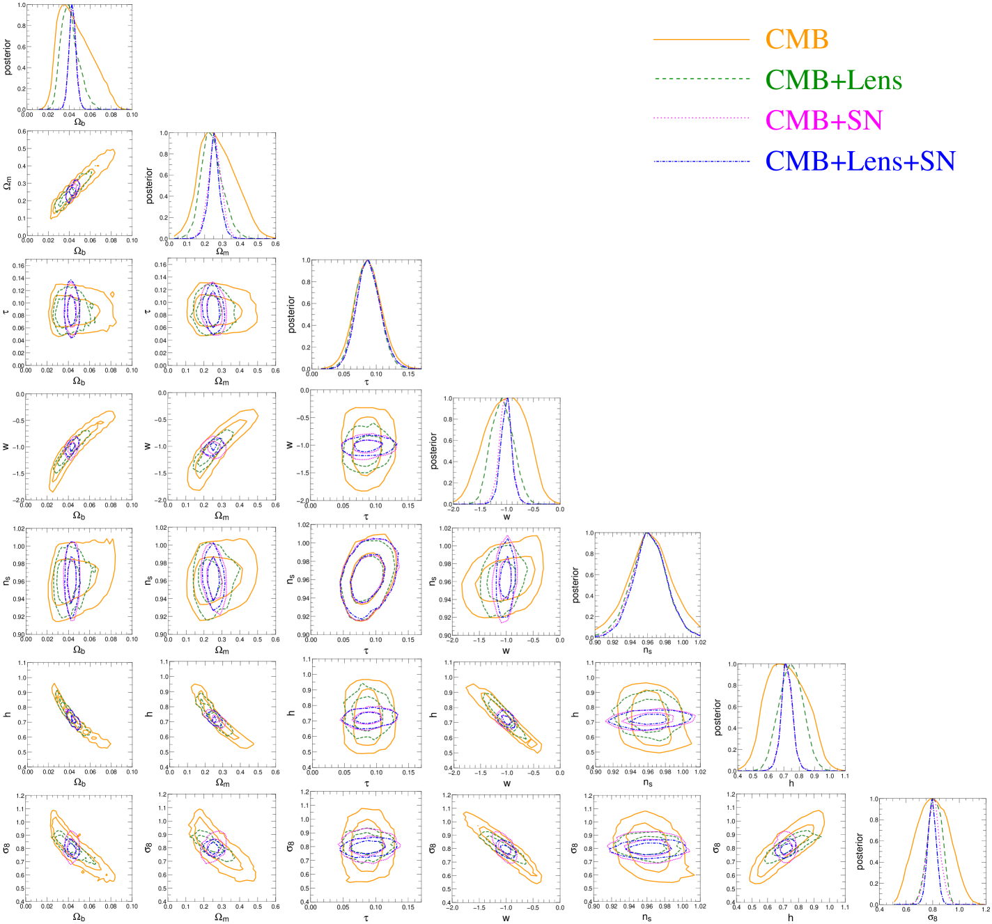
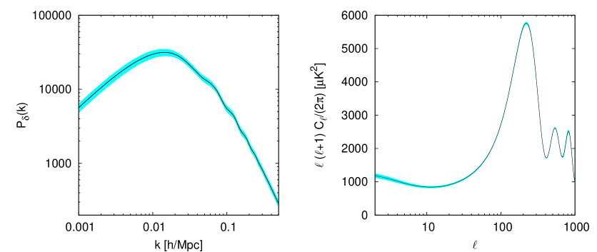
We will now discuss the main results of this paper. Joint constraints using lensing, SNIa and CMB are compared for the two cases with and without taking systematics into account. In the former, both lensing and supernovae systematics are included. The results are given in Table 5, Fig. 8 and Fig. 9. We show the best-fit angular and 3d power spectra in Fig. 10. A CAMB parameter file with our best-fit parameter values is available for download999http://www2.iap.fr/users/kilbinge/params.ini.
With the current data, SNIa is more efficient than lensing in helping decrease uncertainties. CMB+SNIa gives nearly as tight constraints as CMB+SNIa+lensing for most parameters. The reason is that SNIa data show different degeneracy directions, in particular for the pair - (see right panel of Fig. 4). This helps to pin down and thus, the main degeneracy for CMB is largely lifted. As stated in the previous section, this is not the case for lensing — lensing without tomography cannot constrain . The consequence is that even parameters to which SNIa is not sensitive, e.g. , are very accurately determined for the combination CMB+SNIa.
Nevertheless, lensing improves constraints from WMAP5 substantially. Some CMB-related near-degeneracies which arise in the CDM model are partially lifted in combination with lensing. In particular for (), there is a large gain when lensing data is added.
The effect of systematics on the parameters means and errors can be assessed by comparing the last two columns of Table 5. The shift of the best-fit values is less than 15% of the statistical error in all cases. Including systematics in the analysis increases the error bars by 10%-35%, where , and are affected most. Varying the lensing redshift for the bias from 1.0 to 0.8 and 1.2 changes the results by less then one percent.
4 Discussion
In this paper we combine three different cosmological probes to test a possible deviation from a cosmological constant: (1) Weak gravitational lensing as a probe of structure formation and geometry in the redshift range of about to . (2) Supernovae Ia as standard(isable) candles up to redshift unity. (3) CMB anisotropies supplying a wealth of information of the recombination era () and, to a lesser extend, of the Universe up to the re-ionisation epoch (). The data sets are (1) CFHTLS-Wide T0003 (see F08), (2) SNLS first-year (A06) and (3) WMAP five-year (H09), respectively.
We test models in the context of a flat CDM cosmology with a dark- or vacuum-energy component with free but constant equation-of-state parameter . This corresponds to the simplest extension of the ‘vanilla’ CDM model which goes beyond a cosmological constant.
The joint constraints including the modelled systematics in the data sets are (68% and 95% confidence, respectively). Without taking the systematics into account, the result is , representing 25% smaller error bars. With the current data there is no evidence for a dynamical dark-energy component not being the cosmological constant.
Two potential sources of bias in the third-year CFHTLS-Wide lensing data are scrutinised. One, the measured variations of the shear signal (aperture-mass dispersion ) between MegaCam pointings are compared to -body simulations. We estimate the measured fluctuations to be higher than expected by not more than about 5% to 15% on scales below 30 arc minutes. Whereas this might be a hint of systematics in the data, it is not straightforward to model and to assess its effect on cosmology. The second issue are systematics in the shape measurements which seem to lead to an underestimation of the lensing signal at high redshift. We devised a very simple model of this potential systematics by multiplying the lensing efficiency above with a constant , to mimic the effect of a decreased measured shear. Marginalising over cosmological parameters, using weak lensing alone, yields . All probes combined do not constrain much better, we find . Restricting ourselves to , implying an underestimation of the lensing signal, increases by about 8% for a fixed , which is roughly equal to the statistical error. Therefore, in the framework of this simple model, the value of might be biased by 8% if this effect is ignored (as it has been in F08).
Combining all probes we assess the influence of systematics on the cosmological results. The contribution of systematics to the total error budget ranges between 5% and 40% (Table 5). The parameters which are affected most by systematics are and for which this contribution is greater than 20%. Those are the parameters for which weak lensing adds significantly to the joint constraints.
There are indications of more unaccounted systematics in the lensing data. Discussions about the origin of those systematics and ways to remove them are addressed elsewhere (van Waerbeke et al. in prep.). Our findings strengthen the confidence in cosmological results from cosmic shear, presented in this work and earlier, using the same data, in F08.
Our constraints are slightly tighter than Seljak et al. (2005) who obtained using WMAP1, SNIa and, as probes of structure formation, SDSS galaxy correlations and Ly forest clustering. Similar constraints were quoted in Wang & Mukherjee (2006), from WMAP3, SNLS and SDSS. Our results are comparable to the ones stated by Komatsu et al. (2009), (95%) stemming from WMAP5, BAO and SNIa. Consistency is also achieved with the constraints from Mantz et al. (2008) who combined WMAP5 with the X-ray cluster mass function, cluster baryon fraction and SNIa to get (68.3%).
Earlier results including weak gravitational lensing used less wide and/or more shallow data. Using the first-year release of the CFHTLS (T0001, Hoekstra et al. 2006), and with rather tight priors on other cosmological parameters, an upper bound of was derived. Jarvis et al. (2006) combined weak lensing from the 75 deg2 CTIO survey with SNIa and CMB and obtained . The error estimate for the latter includes statistical uncertainty, PSF systematics and shape measurement calibration biases.
This paper puts particular emphasis on the treatment of systematics in the data. Known observation-related systematics are parametrised if possible and included in the analysis together with cosmological parameters. This allows us to directly quantify the influence of systematics on cosmology and to find possible correlations. For SNIa, we calculate the response of the distance modulus to fluctuations of the photometry zero-points. Ignoring these error sources leads to an underestimation of the parameter errors by 10%. The parameter values itself are biased by a fraction of 10% to 20% of the statistical uncertainty.
5 Outlook
For future, high-precision experiments it will be of great importance to understand and control systematic effects. In particular for exotic models, such as time-varying dark-energy or modifications of GR, more and more subtle influences of systematics mimicking a signal have to be excluded. This calls for combined analyses of cosmological and systematics parameters.
Weak lensing serves as an important and independent probe of . The measurement of the lensing skewness will allow us to lift degeneracies between parameters, in particular between and (Kilbinger & Schneider 2005). Power and bi-spectrum tomography can be used to constrain the time-evolution of the dark-energy eos parameter (Takada & Jain 2004). In addition, as a complementary and nearly independent probe of the non-Gaussian, high-density regime of the large-scale structure, weak lensing cluster counts can improve dark-energy parameter constraints (Takada & Bridle 2007).
For lensing, systematic effects which have to be taken into account for future analyses include measurement errors (galaxy shapes, PSF correction, photo-’s), astrophysical sources (intrinsic alignments, source clustering) and theoretical uncertainties (non-linear and baryonic physics). The modelling of all those effects, as suggested recently by Bernstein (2008), leads to a huge number of parameters, on the order of several dozens to hundreds, depending on the number of redshift bins. In case of simultaneous determination of cosmic shear and intrinsic alignments a high number of redshift bins is required (Bridle & King 2007; Joachimi & Schneider 2008).
Already with the present data, more general models of dark energy can be constrained. A wide variety of such models are tested with recent SNIa data (Rubin et al. 2008). Because dark energy and modified gravity can influence distances in a non-distinguishable way, it is important to include measures of the growth of structure. A survey like the CFHTLS-Wide reaches out into the linear regime and is less prone to small-scale uncertainties due to baryonic and non-linear physics, which makes such a survey an excellent probe of the present acceleration of the Universe.
Acknowledgements.
We acknowledge the use of the Legacy Archive for Microwave Background Data Analysis (LAMBDA). Support for LAMBDA is provided by the NASA Office of Space Science. We thank the Terapix group for support and computational facilities. We acknowledge the CFHTLS lensing systematics collaboration for uncovering the weak-lensing systematics that are parametrised and marginalised over in this analysis. We thank O. Cappé, J.-F. Cardoso and O. Doré for helpful discussions, and E. Bertin, S. Prunet and B. Rowe for valuable comments on the manuscript. We also would like to thank the anonymous referee for helpful suggestions which improved the paper. MK is supported by the CNRS ANR “ECOSSTAT”, contract number ANR-05-BLAN-0283-04. IT and LF acknowledge the support of the European Commission Programme 6-th framework, Marie Curie Training and Research Network “DUEL”, contract number MRTN-CT-2006-036133.References
- Astier et al. (2006) Astier, P., Guy, J., Regnault, N., et al. 2006, A&A, 447, 31
- Bartelmann et al. (2006) Bartelmann, M., Doran, M., & Wetterich, C. 2006, A&A, 454, 27
- Benjamin et al. (2007) Benjamin, J., Heymans, C., Semboloni, E., et al. 2007, MNRAS, 381, 702
- Bernstein (2008) Bernstein, G. M. 2008, submitted to ApJ, also arXiv:0808.3400
- Blake & Glazebrook (2003) Blake, C. & Glazebrook, K. 2003, ApJ, 594, 665
- Bridle & King (2007) Bridle, S. & King, L. 2007, New Journal of Physics, 9, 444
- Cappé et al. (2007) Cappé, O., Douc, R., Guillin, A., Marin, J.-M., & Robert, C. 2007, to appear in Statistics and Computing, also arXiv:0710.4242
- Cappé et al. (2004) Cappé, O., Guillin, A., Marin, J.-M., & Robert, C. 2004, J. Comput. Graph. Statist., 13, 907
- Contaldi et al. (2003) Contaldi, C. R., Hoekstra, H., & Lewis, A. 2003, Physical Review Letters, 90, 221303/1
- Coupon et al. (2009) Coupon, J., Ilbert, O., Kilbinger, M., et al. 2009, accepted by A&A, also arXiv:0811.3326
- Dunkley et al. (2005) Dunkley, J., Bucher, M., Ferreira, P. G., Moodley, K., & Skordis, C. 2005, MNRAS, 356, 925
- Dunkley et al. (2009) Dunkley, J., Komatsu, E., Nolta, M. R., et al. 2009, ApJS, 180, 306
- Eifler et al. (2008) Eifler, T., Schneider, P., & Hartlap, J. 2008, submitted to A&A, also arXiv:0810.4254
- Francis et al. (2009) Francis, M. J., Lewis, G. F., & Linder, E. V. 2009, MNRAS, 394, 605
- Frieman et al. (2003) Frieman, J. A., Huterer, D., Linder, E. V., & Turner, M. S. 2003, Phys. Rev. D, 67, 083505
- Fu (2008) Fu, L. 2008, PhD thesis, Université Paris 6
- Fu et al. (2008) Fu, L., Semboloni, E., Hoekstra, H., et al. 2008, A&A, 479, 9
- Gong et al. (2008) Gong, Y., Zhang, T.-J., Lan, T., & Chen, X.-L. 2008, arXiv:0810.3572
- Hamana & Mellier (2001) Hamana, T. & Mellier, Y. 2001, MNRAS, 327, 169
- Hanson & Cunningham (1998) Hanson, K. M. & Cunningham, G. S. 1998, in Medical Imaging: Image Processing, 371–382
- Hastings (1970) Hastings, W. K. 1970, Biometrika, 57, 97
- Heymans et al. (2006) Heymans, C., Van Waerbeke, L., Bacon, D., et al. 2006, MNRAS, 368, 1323
- Hinshaw et al. (2007) Hinshaw, G., Nolta, M. R., Bennett, C. L., et al. 2007, ApJS, 170, 288
- Hinshaw et al. (2009) Hinshaw, G., Weiland, J. L., Hill, R. S., et al. 2009, ApJS, 180, 225
- Hoekstra et al. (2006) Hoekstra, H., Mellier, Y., van Waerbeke, L., et al. 2006, ApJ, 457, 116
- Hoekstra et al. (2002) Hoekstra, H., Yee, H. K. C., & Gladders, M. D. 2002, ApJ, 577, 595
- Ichiki et al. (2009) Ichiki, K., Takada, M., & Takahashi, T. 2009, Phys. Rev. D, 79, 023520
- Ilbert et al. (2006) Ilbert, O., Arnouts, S., McCracken, H. J., et al. 2006, A&A, 457, 841
- Jain & Zhang (2008) Jain, B. & Zhang, P. 2008, Phys. Rev. D, 78, 063503
- Jarvis et al. (2006) Jarvis, M., Jain, B., Bernstein, G., & Dolney, D. 2006, ApJ, 644, 71
- Joachimi & Schneider (2008) Joachimi, B. & Schneider, P. 2008, A&A, 488, 829
- Kaiser (1992) Kaiser, N. 1992, ApJ, 388, 272
- Kilbinger & Munshi (2006) Kilbinger, M. & Munshi, D. 2006, MNRAS, 366, 983
- Kilbinger & Schneider (2005) Kilbinger, M. & Schneider, P. 2005, A&A, 442, 69
- Komatsu et al. (2009) Komatsu, E., Dunkley, J., Nolta, M. R., et al. 2009, ApJS, 180, 330
- Kowalski et al. (2008) Kowalski, M., Rubin, D., Aldering, G., et al. 2008, ApJ, 686, 749
- Lesgourgues et al. (2007) Lesgourgues, J., Viel, M., Haehnelt, M. G., & Massey, R. 2007, Journal of Cosmology and Astro-Particle Physics, 11, 8
- Lewis et al. (2000) Lewis, A., Challinor, A., & Lasenby, A. 2000, Astrophys. J., 538, 473
- Ma (2007) Ma, Z. 2007, ApJ, 665, 887
- Mangano et al. (2002) Mangano, G., Miele, G., Pastor, S., & Peloso, M. 2002, Physics Letters B, 534, 8
- Mantz et al. (2008) Mantz, A., Allen, S. W., Ebeling, H., & Rapetti, D. 2008, MNRAS, 387, 1179
- Martel & Premadi (2008) Martel, H. & Premadi, P. 2008, ApJ, 673, 657
- Massey et al. (2007) Massey, R., Heymans, C., Bergé, J., et al. 2007, MNRAS, 376, 13
- Ménard & Dalal (2005) Ménard, B. & Dalal, N. 2005, MNRAS, 358, 101
- Metropolis et al. (1953) Metropolis, N., Rosenbluth, A., Rosenbluth, M., Teller, A., & Teller, E. 1953, J. Chem. Phys., 21, 1087
- Page et al. (2007) Page, L., Hinshaw, G., Komatsu, E., et al. 2007, ApJS, 170, 335
- Peacock & Dodds (1996) Peacock, J. A. & Dodds, S. J. 1996, MNRAS, 280, L19
- Press et al. (1992) Press, W. H., Teukolsky, S. A., Flannery, B. P., & Vetterling, W. T. 1992, Numerical Recipes in C (Cambridge University Press)
- Rubin et al. (2008) Rubin, D., Linder, E. V., Kowalski, M., et al. 2008, ArXiv e-prints
- Schimd et al. (2007) Schimd, C., Tereno, I., Uzan, J.-P., et al. 2007, A&A, 463, 405
- Schneider et al. (1998) Schneider, P., van Waerbeke, L., Jain, B., & Kruse, G. 1998, MNRAS, 296, 873
- Seljak et al. (2005) Seljak, U., Makarov, A., McDonald, P., et al. 2005, Phys. Rev. D, 71, 103515
- Seo & Eisenstein (2003) Seo, H.-J. & Eisenstein, D. J. 2003, ApJ, 598, 720
- Smith et al. (2003) Smith, R. E., Peacock, J. A., Jenkins, A., et al. 2003, MNRAS, 341, 1311
- Taburet et al. (2009) Taburet, N., Aghanim, N., Douspis, M., & Langer, M. 2009, MNRAS, 392, 1153
- Takada & Bridle (2007) Takada, M. & Bridle, S. 2007, New Journal of Physics, 9, 446
- Takada & Jain (2004) Takada, M. & Jain, B. 2004, MNRAS, 348, 897
- Tereno et al. (2005) Tereno, I., Doré, O., van Waerbeke, L., & Mellier, Y. 2005, A&A, 429, 383
- Tereno et al. (2008) Tereno, I., Schimd, C., Uzan, J.-P., Kilbinger, M. Vincent, F., & Fu, L. 2008, accepted by A&A, also arXiv:0810.0555
- van Waerbeke et al. (2006) van Waerbeke, L., White, M., Hoekstra, H., & Heymans, C. 2006, Astroparticle Physics, 26, 91
- Wang & Mukherjee (2006) Wang, Y. & Mukherjee, P. 2006, ApJ, 650, 1
- Wraith et al. (2009) Wraith, D., Kilbinger, M., Benabed, K., et al. 2009, submitted to Phys. Rev. D, also arXiv:0903.0837
- Xia et al. (2008) Xia, J.-Q., Li, H., Zhao, G.-B., & Zhang, X. 2008, Phys. Rev. D, 78, 083524
- Yahagi (2005) Yahagi, H. 2005, PASJ, 57, 779
- Yahagi & Yoshii (2001) Yahagi, H. & Yoshii, Y. 2001, ApJ, 558, 463