Cluster Monte Carlo and numerical mean field analysis for the water liquid–liquid phase transition

Abstract

By the Wolff’s cluster Monte Carlo simulations and numerical minimization within a mean field approach, we study the low temperature phase diagram of water, adopting a cell model that reproduces the known properties of water in its fluid phases. Both methods allows us to study the water thermodynamic behavior at temperatures where other numerical approaches –both Monte Carlo and molecular dynamics– are seriously hampered by the large increase of the correlation times. The cluster algorithm also allows us to emphasize that the liquid–liquid phase transition corresponds to the percolation transition of tetrahedrally ordered water molecules.

I Introduction

Water is possibly the most important liquid for life sitges and, at the same time, is a very peculiar liquid Debenedetti-JPCM03 . In the stable liquid regime its thermodynamic response functions behave qualitatively differently than a typical liquid. The isothermal compressibility $K_{T}$, for example, has a minimum as a function of temperature at $T=46~{}^{\circ}$C, while for a typical liquid $K_{T}$ monotonically decreases upon cooling. Water’s anomalies become even more pronounced as the system is cooled below the melting point and enters the metastable supercooled regime DebenedettiStanley .

Different hypothesis have been proposed to rationalize the anomalies of water Franzese-JPCM08 . All these interpretations, but one, predict the existence of a liquid–liquid phase transition in the supercooled state, consistent with the experiments to date Franzese-JPCM08 and supported by different models Debenedetti-JPCM03 .

To discriminate among the different interpretations, many experiments have been performed angell2008 . However, the freezing in the temperature-range of interest can be avoided only for water in confined geometries or on the surface of macromolecules Franzese-JPCM08 ; Stanley_etal . Since experiments in the supercooled region are difficult to perform, numerical simulations have played an important role in recent years to help interpret the data. However, also the simulations at very low temperature $T$ are hampered by the glassy dynamics of the empirical models of water slow ; kfsPRL2008 . For these reasons is important to implement more efficient numerical simulations for simple models, able to capture the fundamental physics of water but also less computationally expensive. Here we introduce the implementation of a Wolff’s cluster algorithm wolff for the Monte Carlo (MC) simulations of a cell model for water fs . The model is able to reproduce all the different scenarios proposed to interpret the behavior of water kevin and has been analyzed (i) with mean field (MF) fs ; Franzese-JPCM07 ; kumar-JPCM08 , (ii) with Metropolis MC simulations fmsPRE03 ; kfsPRL2008 and (iii) with Wang-Landau MC density of state algorithm marques-PRE07 . Recent Metropolis MC simulations kfsPRL2008 have shown that very large times are needed to equilibrate the system as $T\rightarrow 0$, as a consequence of the onset of the glassy dynamics. The implementation of the Wolff’s clusters MC dynamics, presented here, allows us to (i) drastically reduce the equilibration times of the model at very low $T$ and (ii) give a geometrical characterization of the regions of correlated water molecules (clusters) at low $T$ and show that the liquid–liquid phase transition can be interpreted as a percolation transition of the tetrahedrally ordered clusters.

Figure 1: A pictorial representation of five water molecules in 3$d$. Two hydrogen bonds (grey links) connect the hydrogens (in blue) of the central molecule with the lone electrons (small gray lines) of two nearest neighbor (n.n.) molecules. A bond index (arm) with $q=6$ possible values is associated to each hydrogen and lone electron, giving rise to $q^{4}$ possible orientational states for each molecule. A hydrogen bond can be formed only if the two facing arms of the n.n. molecules are in the same state. Arms on the same molecule interact among themselves to mimic the O-O-O interaction that drives the molecules toward a tetrahedral local structure.

II The model

The system consists of $N$ particles distributed within a volume $V$ in $d$ dimensions. The volume is divided into $N$ cells of volume $v_{i}$ with $i\in[1,N]$. For sake of simplicity, these cells are chosen of the same size, $v_{i}=V/N$, but the generalization to the case in which the volume can change without changes in the topology of the nearest–neighbor (n.n.) is straightforward. By definition, $v_{i}\geq v_{0}$, where $v_{0}$ is the molecule hard-core volume. Each cell has a variable $n_{i}=0$ for a gas-like or $n_{i}=1$ for a liquid-like cell. We partition the total volume in a way such that each cell has at least four n.n. cells, e.g. as in a cubic lattice in 3$d$ or a square lattice in 2$d$. Periodic boundary conditions are used to limit finite–size effects.

The system is described by the Hamiltonian fs

$$\mathscr{H}=-\epsilon\sum_{\langle i,j\rangle}n_{i}n_{j}-J\sum_{\langle ij\rangle}n_{i}n_{j}\delta_{\sigma_{ij},\sigma_{ji}}+\\ -J_{\sigma}\sum_{i}n_{i}\sum_{(k,l)_{i}}\delta_{\sigma_{ik},\sigma_{il}},$$ (1)

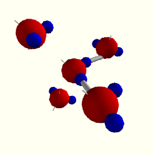
where $\epsilon>0$ is the strength of the van der Waals attraction, $J>0$ accounts for the hydrogen bond energy, with four (Potts) variables $\sigma_{ij}=1,\ldots,q$ representing bond indices of molecule $i$ with respect to the four n.n. molecules $j$, $\delta_{a,b}=1$ if $a=b$ and $\delta_{a,b}=0$ otherwise, and $\langle i,j\rangle$ denotes that $i$ and $j$ are n.n. The model does not assume a privileged state for bond formation. Any time two facing bond indices (arms) are in the same (Potts) state, a bond is formed. The third term represents an intramolecular (IM) interaction accounting for the O–O–O correlation Ricci-Chaplin , locally driving the molecules toward a tetrahedral configuration. When the bond indices of a molecule are in the same state, the energy is decreased by an amount $J_{\sigma}\geqslant 0$ and we associate this local ordered configuration to a local tetrahedral arrangement note . The notation $(k,l)_{i}$ indicates one of the six different pairs of the four bond indices of molecule $i$ (Fig.1).

Experiments show that the formation of a hydrogen bond leads to a local volume expansion Debenedetti-JPCM03 . Thus in our system the total volume is

$$V=Nv_{0}+N_{HB}v_{HB},$$ (2)

where

$$N_{HB}\equiv\sum_{<i,j>}n_{i}n_{j}\delta_{\sigma_{ij},\sigma_{ji}}$$ (3)

is the total number of hydrogen bonds, and $v_{HB}$ is the constant specific volume increase due to the hydrogen bond formation.

III Mean–field analysis

In the mean–field (MF) analysis the macrostate of the system in equilibrium at constant pressure $P$ and temperature $T$ ($NPT$ ensemble) may be determined by a minimization of the Gibbs free energy per molecule, $g\equiv(\langle\mathscr{H}\rangle+PV-TS)/N_{w}$, where

$$N_{w}=\sum_{i}n_{i}$$ (4)

is the total number of liquid-like cells, and $S=S_{n}+S_{\sigma}$ is the sum of the entropy $S_{n}$ over the variables $n_{i}$ and the entropy $S_{\sigma}$ over the variables $\sigma_{ij}$.

A MF approach consists of writing $g$ explicitly using the approximations

$$\sum_{<ij>}n_{i}n_{j} \longrightarrow 2Nn^{2}$$ (5)

$$\sum_{<ij>}n_{i}n_{j}\delta_{\sigma_{ij},\sigma_{ji}} \longrightarrow 2Nn^{2}p_{\sigma}$$ (6)

$$\sum_{i}n_{i}\sum_{(k,l)_{i}}\delta_{\sigma_{ik},\sigma_{il}} \longrightarrow 6Nnp_{\sigma}$$ (7)

where $n=N_{w}/N$ is the average of $n_{i}$, and $p_{\sigma}$ is the probability that two adjacent bond indices $\sigma_{ij}$ are in the appropriate state to form a hydrogen bond.

Therefore, in this approximation we can write

$$V =Nv_{0}+2Nn^{2}p_{\sigma}v_{HB},$$ (8)

$$\langle\mathscr{H}\rangle =-2\left[\epsilon n+\left(Jn+3J_{\sigma}\right)p_{\sigma}\right]nN.$$ (9)

The probability $p_{\sigma}$, properly defined as the thermodynamic average over the whole system, is approximated as the average over two neighboring molecules, under the effect of the mean-field $h$ of the surrounding molecules

$$p_{\sigma}=\left<\delta_{\sigma_{ij},\sigma_{ji}}\right>_{h}.$$ (10)

The ground state of the system consists of all $N$ variables $n_{i}=1$, and all $\sigma_{ij}$ in the same state. At low temperatures, the symmetry will remain broken, with the majority of the $\sigma_{ij}$ in the preferred state. We associate this preferred state to the tetrahedral order of the molecules and define $m_{\sigma}$ as the density of the bond indices in the tetrahedral state, with $0\leq m_{\sigma}\leq 1$. Therefore, the number density $n_{\sigma}$ of bond indices $\sigma_{ij}$ is in the tetrahedral state is

$$n_{\sigma}={{1+(q-1)m_{\sigma}}\over q}.$$ (11)

Since an appropriate form for $h$ is fs

$$h=3J_{\sigma}n_{\sigma},$$ (12)

we obtain that ${{3J_{\sigma}}\over q}\leq h\leq 3J_{\sigma}$.

The MF expressions for the entropies $S_{n}$ of the $N$ variables $n_{i}$, and $S_{\sigma}$ of the $4Nn$ variables $\sigma_{ij}$, are then Franzese-JPCM07

$$S_{n}=-k_{B}N(n\log(n)+(1-n)\log(1-n))$$ (13)

$$S_{\sigma}=-k_{B}4Nn[n_{\sigma}\log(n_{\sigma})+\\ (1-n_{\sigma})\log(1-n_{\sigma})+\log(q-1)],$$ (14)

where $k_{B}$ is the Boltzmann constant.

Equating

$$p_{\sigma}\equiv n_{\sigma}^{2}+{{(1-n_{\sigma})^{2}}\over{q-1}},$$ (15)

with the approximate expression in Eq. (10), allows for solution of $n_{\sigma}$, and hence $g$, in terms of the order parameter $m_{\sigma}$ and $n$.

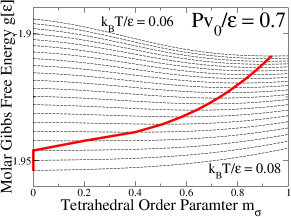
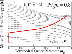
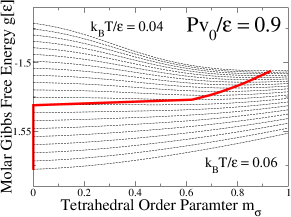
By minimizing numerically the MF expression of $g$ with respect to $n$ and $m_{\sigma}$, we find the equilibrium values $n^{(eq)}$ and $m_{\sigma}^{(eq)}$ and, with Eqs. (4) and (2), we calculate the density $\rho$ at any $(T,P)$ and the full equation of state. An example of minimization of $g$ is presented in Fig. 2 where, for the model’s parameters $J/\epsilon=0.5$, $J_{\sigma}/\epsilon=0.05$, $v_{HB}/v_{0}=0.5$, $q=6$, a discontinuity in $m_{\sigma}^{(eq)}$ is observed for $Pv_{0}/\epsilon>0.8$. As discussed in Ref.s fs ; fmsPRE03 this discontinuity corresponds to a first order phase transition between two liquid phases with different degree of tetrahedral order and, as a consequence, different density. The higher $P$ at which the change in $m_{\sigma}^{(eq)}$ is continuous, corresponds to the pressure of a liquid–liquid critical point (LLCP). The occurrence of the LLCP is consistent with one of the possible interpretations of the anomalies of water, as discussed in Ref. Franzese-JPCM07 . However, for different choices of parameters, the model reproduces also the other proposed scenarios kevin .

Figure 2: Numerical minimization of the molar Gibbs free energy $g$ in the mean field approach. The model’s parameters are $J/\epsilon=0.5$, $J_{\sigma}/\epsilon=0.05$, $v_{HB}/v_{0}=0.5$ and $q=6$. In each panel we present $g$ (dashed lines) calculated at constant $P$ and different values of $T$. The thick line crossing the dashed lines connects the minima $m_{\sigma}^{(eq)}$ of $g$ at different $T$. Upper panel: $Pv_{0}/\epsilon=0.7$, for $T$ going from $k_{B}T/\epsilon=0.06$ (top) to $k_{B}T/\epsilon=0.08$ (bottom). Middle panel: $Pv_{0}/\epsilon=0.8$, for $T$ going from $k_{B}T/\epsilon=0.05$ (top) to $k_{B}T/\epsilon=0.07$ (bottom). Lower panel: $Pv_{0}/\epsilon=0.9$, for $T$ going from $k_{B}T/\epsilon=0.04$ (top) to $k_{B}T/\epsilon=0.06$ (bottom). In each panel dashed lines are separated by $k_{B}\delta T/\epsilon=0.001$. In all the panels $m_{\sigma}^{(eq)}$ increases when $T$ decreases, being 0 (marking the absence of tetrahedral order) at the higher temperatures and $\simeq 0.9$ (high tetrahedral order) at the lowest temperature. By changing $T$, $m_{\sigma}^{(eq)}$ changes in a continuous way for $Pv_{0}/\epsilon=0.7$ and $0.8$, but discontinuous for $Pv_{0}/\epsilon=0.9$ and higher $P$.

IV The simulation with the Wolff’s clusters Monte Carlo algorithm

To perform MC simulations in the $NPT$ ensemble, we consider a modified version of the model in which we allow for continuous volume fluctuations. To this goal, (i) we assume that the system is homogeneous with all the variables $n_{i}$ set to 1 and all the cells with volume $v=V/N$; (ii) we consider that $V\equiv V_{MC}+N_{HB}v_{HB}$, where $V_{MC}\geqslant Nv_{0}$ is a dynamical variable allowed to fluctuate in the simulations; (iii) we replace the first (van der Waals) term of the Hamiltonian in Eq. (1) with a Lennard-Jones potential with attractive energy $\epsilon>J$ and truncated at the hard-core distance

$$U_{W}(r)\equiv\begin{cases}\infty&\text{if $r\leqslant r_{0}$,}\\ \epsilon\left[\left(\frac{r_{0}}{r}\right)^{12}-\left(\frac{r_{0}}{r}\right)^{6}\right]&\text{if $r>r_{0}$.}\\ \end{cases}$$ (16)

where $r_{0}\equiv(v_{0})^{1/d}$; the distance between two n.n. molecules is $(V/N)^{1/d}$, and the distance $r$ between two generic molecules is the Cartesian distance between the center of the cells in which they are included.

The simplification (i) could be removed, by allowing the cells to assume different volumes $v_{i}$ and keeping fixed the number of possible n.n. cells. However, the results of the model under the simplification (i) compares well with experiments Franzese-JPCM07 . Furthermore, the simplification (i) allows to drastically reduce the computational cost of the evaluation of the $U_{W}(r)$ term from $N(N-1)$ to $N-1$ operations. The changes (i)–(iii) modify the model used for the mean field analysis and allow off-lattice MC simulations for a cell model in which the topology of the molecules (i.e. the number of n.n.) is preserved. The comparison of the mean field results with the MC simulations show that these changes do not modify the physics of the system.

We perform MC simulations with $N=2500$ and $N=10000$ molecules, each with four n.n. molecules, at constant $P$ and $T$, in 2d, and with the same parameters used for the mean field analysis. To each molecules we associate a cell on a square lattice. The Wolff’s algorithm is based on the definition of a cluster of variables chosen in such a way to be thermodynamically correlated clusters ; coniglio . To define the Wolff’s cluster, a bond index (arm) of a molecule is randomly selected; this is the initial element of a stack. The cluster is grown by first checking the remaining arms of the same initial molecule: if they are in the same Potts state, then they are added to the stack with probability $p_{\rm same}\equiv\min\left[1,1-\exp(-\beta J_{\sigma})\right]$ wolff , where $\beta\equiv(k_{B}T)^{-1}$. This choice for the probability $p_{\rm same}$ depends on the interaction $J_{\sigma}$ between two arms on the same molecule and guarantees that the connected arms are thermodynamically correlated coniglio . Next, the arm of a new molecule, facing the initially chosen arm, is considered. To guarantee that connected facing arms correspond to thermodynamically correlated variables, is necessary clusters to link them with the probability $p_{\rm facing}\equiv\min\left[1,1-\exp(-\beta J^{\prime})\right]$ where $J^{\prime}\equiv J-Pv_{HB}$ is the $P$–dependent effective coupling between two facing arms as results from the enthalpy $\mathscr{H}+PV$ of the system. It is important to note that $J^{\prime}$ can be positive or negative depending on $P$. If $J^{\prime}>0$ and the two facing arms are in the same state, then the new arm is added to the stack with probability $p_{\rm facing}$; if $J^{\prime}<0$ and the two facing arms are in different states, then the new arm is added with probability $p_{\rm facing}$ note2 . Only after every possible direction of growth for the cluster has been considered the values of the arms are changed in a stochastic way; again we need to consider two cases: (i) if $J^{\prime}>0$, all arms are set to the same new value

$$\sigma^{\rm new}=\left(\sigma^{\rm old}+\phi\right)\mod q$$ (17)

where $\phi$ is a random integer between 1 and $q$; (ii) if $J^{\prime}<0$, the state of every single arm is changed (rotated) by the same random constant $\phi\in[1,\dots q]$

$$\sigma_{i}^{\rm new}=\left(\sigma_{i}^{\rm old}+\phi\right)\mod q.$$ (18)

In order to implement a constant $P$ ensemble we let the volume fluctuate. A small increment $\Delta r/r_{0}=0.01$ is chosen with uniform random probability and added to the current radius of a cell. The change in volume $\Delta V\equiv V^{\rm new}-V^{\rm old}$ and van der Waals energy $\Delta E_{W}$ is computed and the move is accepted with probability $\min\left(1,\exp\left[-\beta\left(\Delta E_{W}+P\Delta V-T\Delta S\right)\right]\right)$, where $\Delta S\equiv-Nk_{B}\ln(V^{new}/V^{old})$ is the entropic contribution.

V Monte Carlo correlation times

The cluster MC algorithm described in the previous section turns out to be very efficient at low $T$, allowing to study the thermodynamics of deeply supercooled water with quite intriguing results mazza . To estimate the efficiency of the cluster MC dynamics with respect to the standard Metropolis MC dynamics, we evaluate in both dynamics, and compare, the autocorrelation function of the average magnetization per site $M_{i}\equiv\frac{1}{4}\sum_{j}\sigma_{ij}$, where the sum is over the four bonding arms of molecule $i$.

$$C_{M}(t)\equiv\frac{1}{N}\sum_{i}\frac{\langle M_{i}(t_{0}+t)M_{i}(t_{0})\rangle-\langle M_{i}\rangle^{2}}{\langle M_{i}^{2}\rangle-\langle M_{i}\rangle^{2}}.$$ (19)

For sake of simplicity, we define the MC dynamics autocorrelation time $\tau$ as the time, measured in MC steps, when $C_{M}(\tau)=1/e$. Here we define a MC step as $4N$ updates of the bond indices followed by a volume update, i.e. as $4N+1$ steps of the algorithm.

Figure 3: Comparison of the autocorrelation function $C_{M}(t)$ for the Metropolis (circles) and Wolff (squares) implementation of the present model. We show the temperatures $k_{B}T/\epsilon=0.11$ (top panel), $k_{B}T/\epsilon=0.09$ (middle panel), $k_{B}T/\epsilon=0.06$ (bottom panel), along the isobar $Pv_{0}/\epsilon=0.6$ close to the LLCP for $N=50\times 50$.

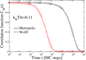
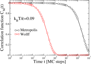
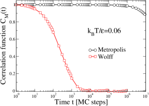
In Fig. 3 we show a comparison of $C_{M}(t)$ for the Metropolis and Wolff algorithm implementations of this model for a system with $N=50\times 50$, at three temperatures along an isobar below the LLCP, and approaching the line of the maximum, but finite, correlation length, also known as Widom line $T_{W}(P)$ Franzese-JPCM07 . In the top panel, at $T\gg T_{W}(P)$ ($k_{B}T/\epsilon=0.11$, $Pv_{0}/\epsilon=0.6$), we find a correlation time for the Wolff’s cluster MC dynamics $\tau_{\rm W}\approx 3\times 10^{3}$, and for the Metropolis dynamics $\tau_{\rm M}\approx 10^{6}$. In the middle panel, at $T>T_{W}(P)$ ($k_{B}T/\epsilon=0.09$, $Pv_{0}/\epsilon=0.6$) the difference between the two correlation times is larger: $\tau_{\rm W}\approx 2.5\times 10^{3}$, $\tau_{\rm M}\approx 3\times 10^{6}$. The bottom panel, at $T\simeq T_{W}(P)$ ($k_{B}T/\epsilon=0.06$, $Pv_{0}/\epsilon=0.6$) shows $\tau_{\rm W}\approx 3.7\times 10^{2}$, while $\tau_{\rm M}$ is beyond the accessible time window ($\tau_{\rm M}>10^{7}$).

Since as $T\rightarrow 0$ the system enters a glassy state kfsPRL2008 , the efficiency $\tau_{\rm M}/\tau_{\rm W}$ grows at lower $T$ allowing the evaluation of thermodynamics averages even at $T\ll T_{C}$ mazza . In particular, the cluster MC algorithm turns out to be very efficient when approaching the Widom line in the vicinity of the LLCP, with an efficiency of the order of $10^{4}$. We plan to analyze in a systematic way how the efficiency $\tau_{\rm M}/\tau_{\rm W}$ grows on approaching the LLCP. This result is well known for the standard liquid-gas critical point wolff and, on the basis of our results, could be extended also to the LLCP. However, this analysis is very expensive in terms of CPU time and goes beyond the goal of the present work. Nevertheless, the percolation analysis, presented in the next section, helps in understanding the physical reason for this large efficiency.

The efficiency is a consequence of the fact that the average size of Wolff’s clusters changes with $T$ and $P$ in the same way as the average size of the regions of correlated molecules coniglio , i.e. a Wolff’s cluster statistically represents a region of correlated molecules. Moreover, the mean cluster size diverges at the critical point with the same exponent of the Potts magnetic susceptibility coniglio , and the clusters percolate at the critical point, as we will discuss in the next section.

VI Percolating clusters of correlated molecules

The efficiency of the Wolff’s cluster algorithm is a consequence of the exact relation between the average size of the finite clusters and the average size of the regions of thermodynamically correlated molecules. The proof of this relation at any $T$ derives straightforward from the proof for the case of Potts variables coniglio . This relation allows to identify the clusters built during the MC dynamics with the correlated regions and emphasizes (i) the appearance of heterogeneities in the structural correlations hetero , and (ii) the onset of percolation of the clusters of tetrahedrally ordered molecules at the LLCP percolation , as shown in Fig. 4.

Figure 4: Three snapshots of the system with $N=100\times 100$, showing the Wolff’s clusters of correlated water molecules. For each molecule we show the states of the four arms and associate different colors to different arm’s states. The state points are at pressure close to the critical value $P_{C}$ ($Pv_{0}/\epsilon=0.72\simeq P_{C}v_{0}/\epsilon$) and $T>T_{C}$ (top panel, $k_{B}T/\epsilon=0.0530$), $T\simeq T_{C}$ (middle panel, $k_{B}T/\epsilon=0.0528$), $T<T_{C}$ (bottom panel, $k_{B}T/\epsilon=0.0520$), showing the onset of the percolation at $T\simeq T_{C}$.

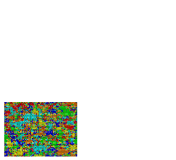
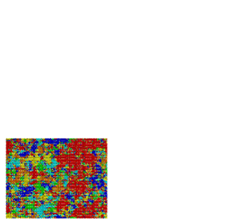
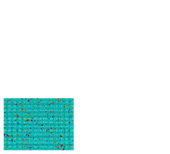
A systematic percolation analysis clusters is beyond the goal of this report, however configurations such as those in Fig. 4 allow the following qualitative considerations. At $T>T_{C}$ the average cluster size is much smaller than the system size. Hence, the structural correlations among the molecules extends only to short distances. This suggests that the correlation time of a local dynamics, such as Metropolis MC or molecular dynamics, would be short on average at this temperature and pressure. Nevertheless, the system appears strongly heterogeneous with the coexistence of large and small clusters, suggesting that the distribution of correlation times evaluated among molecules at a given distance could be strongly heterogeneous. The clusters appear mostly compact but with a fractal surface, suggesting that borders between clusters can rapidly change.

At $T\simeq T_{C}$ there is one large cluster, in red on the right of the middle panel of Fig. 4, with a linear size comparable to the system linear extension and spanning in the vertical direction. The appearance of spanning clusters shows the onset of the percolation geometrical transition. At this state point the correlation time of local, such as Metropolis MC dynamics or molecular dynamics would be very slow as a consequence of the large extension of the structurally correlated region. On the other hand, the correlation time of the Wolff’s cluster dynamics is short because it changes in one single MC step the state of all the molecules in clusters, some of them with very large size. Once the spanning cluster is formed, it breaks the symmetry of the system and a strong effective field acts on the molecules near its border to induce their reorientation toward a tetrahedral configuration with respect the molecules in the spanning cluster.

As shown in Fig.3, the spanning cluster appears as a fractal object, with holes of any size. The same large distribution of sizes characterizes also the finite clusters in the system. The absence of a characteristic size for the clusters (or the holes of the spanning cluster) is the consequence of the fluctuations at any length-scale, typical of a critical point.

At $T<T_{C}$ the majority of the molecules belongs to a single percolating cluster that represents the network of tetrahedrally ordered molecules. All the other clusters are small, with a finite size that corresponds to the regions of correlated molecules. The presence of many small clusters gives a qualitative idea of the heterogeneity of the dynamics at these temperatures.

VII Summary and conclusions

We describe the numerical solution of mean field equations and the implementation of the Wolff’s cluster MC algorithm for a cell model for liquid water. The mean field approach allows us to estimate in an approximate way the phase diagram of the model at any state point predicting intriguing new results at very low $T$ mazza .

To explore the state points of interest for these predictions the use of standard simulations, such as molecular dynamics or Metropolis MC, is not effective due to the onset of the glassy dynamics kfsPRL2008 . To overcome this problem and access the deeply supercooled region of liquid water, we adopt the Wolff’s cluster MC algorithm. This method, indeed, allows to greatly accelerate the autocorrelation time of the system. Direct comparison of Wolff’s dynamics with Metropolis dynamics in the vicinity of the liquid-liquid critical point shows a reduction of the autocorrelation time of a factor at least $10^{4}$.

Furthermore, the analysis of the clusters generated during the Wolff’s MC dynamics allows to emphasize how the regions of tetrahedrally ordered molecules build up on approaching the liquid–liquid critical point, giving rise to the backbone of the tetrahedral hydrogen bond network at the phase transition percolation . The coexistence of clusters of correlated molecules with sizes that change with the state point gives a rationale for the heterogeneous dynamics observed in supercooled water hetero .

VIII Acknowledgments

We thank Andrew Inglis for introducing one of the authors (MGM) to VPython, Francesco Mallamace for discussions, NSF grant CHE0616489 and Spanish MEC grant FIS2007-61433 for support.

References

- (1) Aspects of Physical Biology: Biological Water, Protein Solutions, Transport and Replication, G. Franzese and M. Rubi eds. (Springer, Berlin, 2008).
- (2) P. G. Debenedetti, J. Phys.: Condens. Matter 15 (2003) R1669.
- (3) P. G. Debenedetti and H. E. Stanley, “The Physics of Supercooled and Glassy Water,” Physics Today 56 [issue 6] (2003) 40.
- (4) G. Franzese, K. Stokely, X.-Q. Chu, P .Kumar, M. G. Mazza, S.-H. Chen, and H. E. Stanley, J. Phys.: Condens. Matter 20 (2008) 494210.
- (5) C. A. Angell, Science 319 (2008) 582.
- (6) H.E. Stanley, P. Kumar, G. Franzese, L.M. Xu, Z.Y. Yan, M.G. Mazza, S.-H. Chen, F.Mallamace, S. V. Buldyrev, “Liquid polyamorphism: Some unsolved puzzles of water in bulk, nanoconfined, and biological environments”, in Complex Systems, M. Tokuyama, I. Oppenheim, H. Nishiyama H, eds. AIP Conference Proceedings, 982 (2008) 251.
- (7) H. E. Stanley, S. V. Buldyrev, G. Franzese, N. Giovambattista, F. W. Starr, Phil. Trans. Royal Soc. 363, 509 (2005); P. Kumar, G. Franzese, S. V. Buldyrev, and H. E. Stanley, Phys. Rev. E 73 (2006) 041505.
- (8) P. Kumar, G. Franzese and H. E. Stanley, Phys. Rev. Lett. 100 (2008) 105701.
- (9) U. Wolff, Phys. Rev. Lett. 62 (1989) 361.
- (10) G. Franzese and H. E. Stanley, J. Phys.: Condens. Matter 14 (2002) 2201; Physica A 314 (2002) 508.
- (11) K. Stokely, M. G. Mazza, H. E. Stanley, G. Franzese, “Effect of hydrogen bond cooperativity on the behavior of water” arXiv:0805.3468v1 (2008).
- (12) G. Franzese and H. E. Stanley, J. Phys.: Condens. Matter 19 (2007) 205126.
- (13) P. Kumar, G. Franzese and H. E. Stanley, J. Phys.: Condens. Matter 20 (2008) 244114.
- (14) G. Franzese, M. I. Marqués, and H. Eugene Stanley, Phys. Rev. E 67 (2003) 011103.
- (15) M. I. Marqués, Phys. Rev. E 76 (2007) 021503.
- (16) M.A. Ricci, F. Bruni, and A. Giuliani Similarities between confined and supercooled water, to appear on Faraday Discussion (2008). M. Chaplin “Water’s Hydrogen Bond Strength”, cond-mat/0706.1355 (2007).
- (17) The model does not differentiate “donor” molecule and “acceptor” molecule in the hydrogen bond definition. This simplification increases the number of possible bonded configurations, hence increases the entropy associated to the local tetrahedral configurations. A simple modification of the model could explicitly take into account this feature, however the comparison of the results from the present version of the model with experiments and simulations from more detailed models shows good qualitative agreement.
- (18) V. Cataudella, G. Franzese, M. Nicodemi, A. Scala, and A. Coniglio, Phys. Rev. E 54 (1996) 175; G.Franzese, J. Phys. A 29 (1996) 7367.
- (19) A. Coniglio and F. Peruggi, J. Phys. A 15 (1982) 1873.
- (20) The results of clusters ; coniglio guarantee that the cluster algorithm described here satisfies the detailed balance and is ergodic. Therefore, it is a valid Monte Carlo dynamics.
- (21) M. G. Mazza, K. Stokely, H. E. Stanley, and G. Franzese, “Anomalous specific heat of supercooled water”, cond-mat/0807.4267 (2008).
- (22) M.G. Mazza et al., Phys. Rev. Lett. 96 (2006) 057803; N. Giovambattista et al., J. Phys. Chem. B 108 (2004) 6655; M.G. Mazza et al., Phys. Rev. E 76 (2007) 031203.
- (23) A. Oleinikova, I. Brovchenko, J. Phys.: Condens. Matter 18 (2006) S2247.