Measuring Distance Ratios with CMB-Galaxy Lensing Cross-correlations
Abstract
We propose a method for cosmographic measurements by combining gravitational lensing of the cosmic microwave background (CMB) with cosmic shear surveys. We cross-correlate the galaxy counts in the lens plane with two different source planes: the CMB at and galaxies at an intermediate redshift. The ratio of the galaxy count/CMB lensing cross-correlation to the galaxy count/galaxy lensing cross correlation is shown to be a purely geometric quantity, depending only on the distribution function of the source galaxies. By combining Planck, ADEPT and LSST the ratio can be measured to accuracy, whereas a future polarization based experiment like CMBPOL can make a more precise () measurement. For cosmological models where the curvature and the equation of state parameter are allowed to vary, the direction of degeneracy defined by the measurement of this ratio is different from that traced out by Baryon Acoustic Oscillation (BAO) measurements. Combining this method with the stacked cluster mass reconstruction cosmography technique as proposed by Hu, Holz and Vale (2007), the uncertainty in the ratio can be further reduced, improving the constraints on cosmological parameters. We also study the implications of the lensing-ratio measurement for early dark energy models, in context of the parametrization proposed by Doran and Robbers (2006). For models which are degenerate with respect to the CMB, we find both BAO and lensing-ratio measurements to be insensitive to the early component of the dark energy density.
I Introduction
Weak gravitational lensing of the cosmic microwave background (CMB) (see Lewis and Challinor (2006) for a review) provides us with a unique opportunity to study the large scale distribution of dark matter in the universe out to much greater distances than accessible through conventional galaxy-lensing studies. It has been shown (Jain and Taylor, 2003) that by studying the gravitational lensing of galaxies in different redshift slices by the same foreground structures, the geometry of the universe and eventually, dark energy evolution may be constrained — a method known as cross-correlation cosmography. In this paper, we propose a similar method in which we treat the CMB as one of the background slices. This not only provides an extremely well standardized distance to compare other distances to, but also incorporates the longest possible distance in the ratio of distances probed by this method, making it a more sensitive probe of cosmological parameters than ratios involving distances restricted to galaxy surveys. Recently, Hu et al. (Hu et al., 2007) have proposed a method for measuring the same lensing-ratio by comparing the convergence profile of the a cluster reconstructed via background galaxy shear with that reconstructed via CMB lensing, and then stacking several clusters to improve the precision of the measurement. The method we propose here depend on cross-correlations rather than reconstruction of convergence of individual objects, and will have different systematics. As such, this method is a powerful complement to the cluster-lensing based method and the two may be combined to obtain more precise measurements of the ratio.
II Lensing Ratio: The key observable
Cosmological weak lensing effects are conveniently encoded in the effective convergence field, which is defined as a weighted projection of the matter overdensities (Bartelmann and Schneider, 2001),
| (1) |
with
| (2) |
where is the comoving angular diameter distance corresponding to the comoving distance . Here, is the scale factor, while and represent the present values of the matter density parameter and the Hubble parameter, respectively. The quantity represents the fact that sources are distributed in comoving distance with a normalized distribution function . Since the CMB photons all come from nearly the same cosmological distance, we can approximate the source distribution function as, , giving
| (3) |
where is the comoving distance to the last scattering surface. We will denote the same quantity for a background galaxy population with redshift distribution , with the symbol .
We also consider a suitable foreground population as a tracer of large-scale structure. The projected fractional overdensity of the tracers can be written as,
| (4) |
where represents the fractional tracer overdensity and is the normalized tracer distribution function in comoving distance. We assume that the Fourier modes of the tracer overdensity field are related to those of the underlying matter density field via a scale and redshift dependent bias factor, so that . If we cross-correlate the tracer overdensity map with the convergence field, we obtain the cross power spectrum,
| (5) |
where we have used the Limber approximation and the orthogonality of spherical harmonics. We have also introduced the shorthand notation, .
Now, we will introduce two separate cross-correlation measures involving the foreground tracer population. First, we consider the case for the CMB as the background source. By constructing estimators out of quadratic combinations of CMB fields (temperature and polarization), it possible to obtain a noisy reconstruction of the convergence field (note that the actual observable in this case is the deflection field) out to the last scattering surface (Hu and Okamoto, 2002; Hirata and Seljak, 2003), which we denote as . The power spectrum of the noise in the reconstruction, , can be estimated knowing the specifications for the CMB experiment. The cross-correlation of the reconstructed convergence field from the lensed CMB with the foreground tracer, gives the signal,
| (6) |
where we have used the source distribution kernel appropriate for the CMB being the background source.
Next, we consider the case for the weak lensing of background galaxies. The relevant observable in this case is the traceless symmetric shear field on the sky, the measurement of which allows a noisy reconstruction of the convergence field appropriate to the background galaxy distribution, . In this case, the noise is primarily due to intrinsic ellipticity of the background galaxies and has the spectrum, where and is the number of background galaxies per steradian (Kaiser, 1992). If we cross correlate this convergence field with the foreground tracers, we find the signal,
| (7) |
where we have used the source distribution kernel, appropriate for background galaxies.
If the foreground distribution is narrow in redshift so that it can be approximated by a delta function, , then the ratio of the above two cross-correlation measures, which we call the lensing-ratio, reduces to,
| (8) |
which is simply the geometrical ratio of the source distribution kernels. If the background galaxy distribution, too, is sufficiently narrow in redshift around , this becomes,
| (9) |
Note that this is independent of the angular scale, tracer bias and the power spectrum. Therefore, measurements at several multipoles can be combined to constrain the lensing-ratio. Since the distance ratios depend on the cosmology and specifically on the dark energy model, this can be used to constrain dark energy parameters.
III Upcoming surveys and a new probe of dark energy and curvature
Large scale structure surveys, together with precision measurements of the CMB anisotropies have already provided us with a wealth of knowledge about the geometry, evolution and composition of the Universe. In the coming decade, Cosmologists will carry out even larger scale galaxy and lensing surveys and produce higher resolution CMB maps. We consider a combination of three experiments in order to assess how well the lensing-ratio can be measured in such future surveys. We consider the redshift slice of foreground tracers (lenses) to be drawn from an ADEPT-like 111Advanced Dark Energy Physics Telescope; http://universe.nasa.gov/program/probes/adept.html large scale structure survey and the background (source) galaxies taken from an LSST-like 222Large Synoptic Survey Telescope; http://www.lsst.org weak lensing experiment. For the CMB lensing measurements, we consider the upcoming Planck mission as well as a prospective polarization-based mission like CMBPOL.
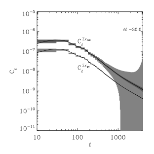
The foreground galaxy slice is taken as a step function in the redshift range with galaxies per square degree. The source galaxies are also assumed to be distributed uniformly in redshift, between and with a number density of galaxies per square arcmin. We model Planck to be a FWHM instrument with temperature and polarization sensitivities of and K-arcmin, respectively. For CMBPOL, we adopt a beam FWHM and temperature and polarization sensitivities of and K-arcmin, respectively. We assume that both CMB experiments cover of the sky and all cross-correlations are performed over the same area. For calculations performed here we assumed a WMAP 5-year normalized CDM cosmology with , , , , and .
In Fig. 1, we display the two cross power spectra appearing in the defining equation 8 of the lensing ratio along with binned uncertainties predicted from the experimental specifications.
The error on the ratio can be obtained as follows. We begin by defining the log-likelihood,
| (10) |
where, . We compute the variance of at the value of computed in the fiducial cosmology,
| (11) | |||||
where,
include the noise power spectra. The Poisson noise for the foreground tracer is taken as . Then maximum likelihood estimate for the ratio is then obtained by solving to be,
| (12) |
Now, we can estimate the error on as,
| (13) |
Various auto, cross and noise power spectra that enter the calculation of the error on are shown in Fig. 2. The above figures borne out the expected feature that the noise power spectrum in the lensing reconstruction is the largest source of uncertainty that propagates into the error on .
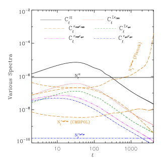
The estimated errors on are shown in Table 1. For Planck, we find that the lensing-ratio can be estimated to while with CMBPOL a measurement is possible.
| Experiment | Type | (S/N)cross | |
|---|---|---|---|
| Planck | POL | 25.8 | 3.8 |
| TT | 23.3 | 4.2 | |
| CMBPOL | POL | 102.6 | 1.0 |
| TT | 84.5 | 1.2 |
IV Parameter constraints
For Planck priors, improvements on cosmological parameter constraints upon adding the lensing-ratio to the primary CMB observables become appreciable when the error on the ratio decreases below (Hu et al., 2007). It is interesting to note here that the method for estimating the lensing-ratio proposed by Hu, Holz and Vale (2007) (Hu et al., 2007), which relies on cluster mass reconstruction can be further improved with the maximum likelihood based estimator proposed by Yoo and Zaldarriaga (Yoo and Zaldarriaga, 2008) and can complement the method proposed here. By combining the two methods for the same redshift slices, it may be possible to reduce the uncertainty in the lensing-ratio to percent or sub-percent levels.
In order to assess how a percent-level measurement of the ratio will help constrain a set of cosmological parameters in conjunction with the CMB experiments, we define a Fisher matrix for the lensing-ratio,
| (14) |
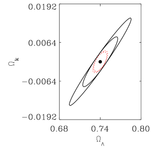
and add it to the Fisher matrix from a CMB experiment. The error in a parameter is then estimated from the inverse of the combined Fisher matrix as . We consider two variants of the CMB Fisher Matrix, one with only the primordial power spectra and the other with the power spectra involving the weak lensing deflection field extracted from CMB lensing measurements (Lesgourgues et al., 2006; Perotto et al., 2006). We do not consider any foreground contamination in any of these. Fig. 3 shows the constraints predicted with Planck specifications and a error on the lensing-ratio, for minimal extensions to the standard 6-parameter model. These constrains are marginalized over all other parameters. The constraints on curvature assuming and on assuming flatness, both improve over the primary CMB case after adding in the ratio. For CMB with lensing extraction the improvement on is still substantial while that on is marginal.
Following Lesgourgues et al. (2006), we also consider a more general 11-parameter model with , fraction of dark matter in massive neutrinos , the effective number of neutrino species, the running of the spectral index and the primordial Helium fraction. We adopt a fiducial value of eV for the total neutrino mass. The constraints on the interesting subspace of parameters are shown in Fig. 4.
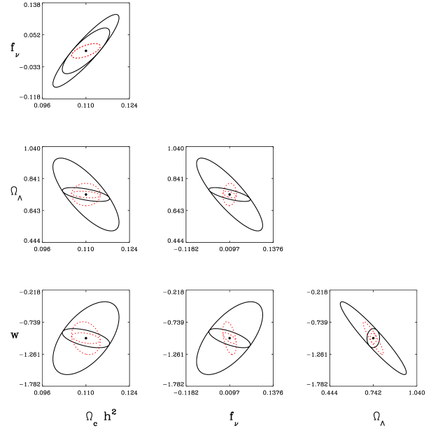
We find in this case that adding in the ratio significantly improves the constraints on and over the primary CMB case. In fact, for and the improvements surpass those from the lensed CMB Fisher matrix. This is particularly interesting because the lensed-CMB-only constraints require an estimate of the convergence field from the four point function in the lensed CMB itself and is more prone to systematics than the cross-correlations that enter the ratio calculation. From Fig. 4, it is apparent that for the CMB Fisher matrix with lensing extraction the constraint on the neutrino mass is rather tight, so that no further gain is obtained by adding in the lensing-ratio. It is important to keep in mind that Fisher matrix methods tend to overestimate the error on neutrino mass due to non-Gaussianity in the associated likelihood (Perotto et al., 2006). Therefore, the errors estimated here are somewhat higher than those predicted from a full Monte-Carlo forecast.

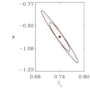
We next consider models with curvature and a free dark energy parameter . CMB measurements allow for a large degenerate valley in the plane making Fisher Matrix results deceptive. We treat this model by imposing a strong CMB prior in which we explore the parameter space while keeping the high-redshift variables , and fixed. For each degenerate parameter set, we calculate the value of as well as the spherically averaged baryon acoustic oscillation (BAO) distance ratio (Percival et al., 2007; Eisenstein et al., 2005), , where is the comoving sound horizon scale at the drag epoch, and is an effective distance measure to redshift . We compute it for , a typical median redshift for an ADEPT-like survey. The constraints in the plane from each of these methods are shown in Fig 5 for a measurement of the BAO ratio with ADEPT (Seo and Eisenstein, 2007) combined with a measurement of the lensing-ratio. We find that the degeneracy direction for the BAO is quite different from that for the lensing-ratio. Together they can put a limit on and a simultaneous limit on , without adding in any other cosmological prior.
Next, we turn to scenarios with early dark energy. In particular, we choose the dark energy parametrization proposed by (Doran and Robbers, 2006), namely,
| (15) |
where is the present value of the dark energy density function, , and is its asymptotic value at high redshift. In this parametrization, the dark energy equation of state has the value at present, crosses over to during matter domination and goes to in the radiation dominated era. Two relations of interest in this model that follow from the definition of the Hubble parameter,
| (16) |
are the scaling, with , of the comoving sound horizon at last scattering or the drag epoch, namely,
| (17) |
and the behavior of the comoving angular diameter distance which, for flat cosmologies, given by,
| (18) |
We consider the parameter space spanned by and study how well it can be constrained given measurements of the lensing ratio, the CMB and the BAO. We again impose the strong CMB prior, and compute the observables for each point in the space degenerate with respect to the CMB. Since early dark energy shifts the comoving sound horizon according to equation 17, and we are fixing the values and (which fixes the redshift of last scatter), equation 18 immediately implies that the only way to keep the angular scale constant is by varying such that scales like . Thus, quite counter-intuitively, we find that the early value of the dark energy indirectly affects low redshift evolution. An unfortunate consequence of this is that both BAO and lensing ratio measurements are rendered insensitive to the value of . As shown by Linder & Robbers (2008), it is possible to have a set of cosmological models degenerate with respect to the CMB without having strictly constant. For example, holding , and therefore constant, it is still possible to have nearly indistinguishable CMB power spectra. In this case, to preserve , one has to change accordingly. This, again, leads to the shift in low redshift distances and makes our observables insensitive to . These issues are discussed in some detail in the Appendix.
V Conclusions
We have proposed a way of measuring a ratio of comoving angular diameter distances that appear in the lensing kernels for CMB and galaxy lensing. By combining Planck, ADEPT and LSST, it is possible make a percent level measurement of this ratio. A polarization based experiment like CMBPOL has the potential of making a more precise measurement. The precision in the measurement can be potentially increased by combining it with cluster mass reconstruction based measurement of the same quantity. The ratio is sensitive to late-time geometry and composition of the Universe and a percent level measurement combined with Planck data can provide interesting constraints and consistency checks, independently of other cosmological probes. By choosing the CMB as one of the lens planes, this method allows higher redshifts to be probed than galaxy-lensing cosmography.
While the distance ratio is sensitive to late time dark energy, we find it to be rather insensitive to early dark energy, particularly for the parametrization proposed in Doran and Robbers (2006). As discussed in the Appendix, when a strong CMB prior is imposed, the values of low redshift parameters shift in conjunction with the asymptotic high redshift value of early dark energy in such a manner as to render both the BAO ratio and the lensing ratio rather insensitive probes. This behavior is most likely a specific feature of the said parametrization. The effectiveness of the lensing ratio as a cosmological tool for a wider class of quintessence models remains to be studied. *
Appendix A BAO and lensing ratios as probes of early dark energy


Let us choose the fiducial dark energy model as one with , and with the other cosmological parameters set at the values described in the body of the paper. Now, if we had wrongly assumed i.e. a model, then by fitting the CMB, we would find a set of parameters that would keep the angle constant. As , we would find a model that overestimates the sound horizon and hence the comoving angular diameter distance to the last scattering surface by the factor i.e. by . In particular, if we also impose the strong constraint that is a constant, this model would have a value of that would be slightly lower than the true value, namely . This would, in turn, make us overestimate the value of to all redshifts (see Fig. 6).
Now consider the BAO ratio at some redshift . For the sound horizon at the drag epoch, we would again make an overestimate by the same factor, . But at the same time, we overestimate or by an almost similar factor because has shifted (see Figs. 6 & Figs. 7). Therefore, the transverse ratio or the line-of-sight ratio estimated in the wrong model will be rather close to the true values, thereby making it hard to detect the presence of early dark energy. In fact, these figures show that deviations from the fiducial ratio occur only at the level at . Because the angular scale of the CMB acoustic peak is a precisely measured quantity, it is expected that even if the strong CMB prior is relaxed, a MCMC type exploration of the parameter space would reveal a similar insensitivity of the BAO to (Doran et al., 2007).
For the lensing ratio, the situation is even worse, as depicted in the right panel of Fig. 7. Here, due to overall shift of all distance scales, the difference between the inferred and the true model is less than at all lens redshifts.


References
- Lewis and Challinor (2006) A. Lewis and A. Challinor, Phys. Rep. 429, 1 (2006), eprint arXiv:astro-ph/0601594.
- Jain and Taylor (2003) B. Jain and A. Taylor, Physical Review Letters 91, 141302 (2003), eprint arXiv:astro-ph/0306046.
- Hu et al. (2007) W. Hu, D. E. Holz, and C. Vale, Phys. Rev. D 76, 127301 (2007), eprint arXiv:0708.4391.
- Bartelmann and Schneider (2001) M. Bartelmann and P. Schneider, Phys. Rep. 340, 291 (2001), eprint arXiv:astro-ph/9912508.
- Hu and Okamoto (2002) W. Hu and T. Okamoto, Astrophys. J. 574, 566 (2002), eprint arXiv:astro-ph/0111606.
- Hirata and Seljak (2003) C. M. Hirata and U. Seljak, Phys. Rev. D 67, 043001 (2003), eprint arXiv:astro-ph/0209489.
- Kaiser (1992) N. Kaiser, Astrophys. J. 388, 272 (1992).
- Yoo and Zaldarriaga (2008) J. Yoo and M. Zaldarriaga, ArXiv e-prints 805 (2008), eprint 0805.2155.
- Lesgourgues et al. (2006) J. Lesgourgues, L. Perotto, S. Pastor, and M. Piat, Phys. Rev. D 73, 045021 (2006), eprint arXiv:astro-ph/0511735.
- Perotto et al. (2006) L. Perotto, J. Lesgourgues, S. Hannestad, H. Tu, and Y. Y Y Wong, Journal of Cosmology and Astro-Particle Physics 10, 13 (2006), eprint arXiv:astro-ph/0606227.
- Percival et al. (2007) W. J. Percival, S. Cole, D. J. Eisenstein, R. C. Nichol, J. A. Peacock, A. C. Pope, and A. S. Szalay, MNRAS 381, 1053 (2007), eprint arXiv:0705.3323.
- Eisenstein et al. (2005) D. J. Eisenstein, I. Zehavi, D. W. Hogg, R. Scoccimarro, M. R. Blanton, R. C. Nichol, R. Scranton, H.-J. Seo, M. Tegmark, Z. Zheng, et al., Astrophys. J. 633, 560 (2005), eprint arXiv:astro-ph/0501171.
- Seo and Eisenstein (2007) H.-J. Seo and D. J. Eisenstein, Astrophys. J. 665, 14 (2007), eprint arXiv:astro-ph/0701079.
- Doran and Robbers (2006) M. Doran and G. Robbers, Journal of Cosmology and Astro-Particle Physics 6, 26 (2006), eprint arXiv:astro-ph/0601544.
- Linder & Robbers (2008) Linder, E. V., & Robbers, G. 2008, Journal of Cosmology and Astro-Particle Physics, 6, 4
- Doran et al. (2007) M. Doran, S. Stern, and E. Thommes, Journal of Cosmology and Astro-Particle Physics 4, 15 (2007), eprint arXiv:astro-ph/0609075.