Monte Carlo Markov Chain Parameter Estimation in Semi-Analytic Models of Galaxy Formation

Abstract

We present a statistical exploration of the parameter space of the De Lucia and Blaizot version of the Munich semi-analytic (SA) model built upon the Millennium dark matter simulation. This is achieved by applying a Monte Carlo Markov Chain method to constrain the 6 free parameters that define the stellar and black-hole mass functions at redshift zero. The model is tested against three different observational data sets, including the galaxy $K$-band luminosity function, $B-V$ colours, and the black hole-bulge mass relation, separately and combined, to obtain mean values, confidence limits and likelihood contours for the best fit model. Using each observational data set independently, we discuss how the SA model parameters affect each galaxy property and find that there are strong correlations between them. We analyse to what extent these are simply reflections of the observational constraints, or whether they can lead to improved understandings of the physics of galaxy formation.

When all the observations are combined, we find reasonable agreement between the majority of the previously published parameter values and our confidence limits. However, the need to suppress dwarf galaxy formation requires the strength of the supernova feedback to be significantly higher in our best-fit solution than in previous work. To balance this, we require the feedback to become ineffective in halos of lower mass than before, so as to permit the formation of sufficient high-luminosity galaxies: unfortunately, this leads to an excess of galaxies around L^∗. Although the best-fit is formally consistent with the data, there is no region of parameter space that reproduces the shape of galaxy luminosity function across the whole magnitude-range.

For our best fit we present the model predictions for the $b_{\rm J}$-band luminosity and stellar mass functions. We find a systematic disagreement between the observed mass function and the predictions from the $K$-band constraint, which we explain in light of recent works that suggest uncertainties of up to 0.3 dex in the mass determination from stellar population synthesis models.

We discuss modifications to the semi-analytic model that might simultaneously improve the fit to the observed mass function and reduce the reliance on excessive supernova feedback in small halos.

1 Introduction

The combination of the well established $\Lambda$CDM paradigm and the geometrical growth of computer power in recent years, has allowed direct N-body simulations to give us a comprehensive picture of the formation and evolution of dark matter structure, from the primordial gravitational instabilities to the formation of massive superclusters today (The Millennium Run, Springel et al., 2005).

However this progress is not reflected in our theoretical understanding of the behaviour of the baryons, with much of the physics governing galaxy formation and evolution still poorly understood. A combined simulation of gas and dark matter resolving small-scale galaxy evolution processes (such as gas cooling, star formation and feedback) over a cosmologically interesting volume is still years away. Therefore the only plausible method to construct a model galaxy population for comparison with observed large-scale surveys is using a semi-analytic formalism. Originally introduced by White & Rees (1978), this formalism treats the dark matter structure using either a Press-Schechter (Press & Schechter, 1974), Monte-Carlo or N-body approach and on top of that follows galaxy evolution using parameterised equations governing the laws of subgrid physics. The basic methodology was set by Cole (1991), Lacey & Silk (1991) and White & Frenk (1991), including the dependence of gas cooling and star formation on the dark matter halo density profile, feedback and chemical enrichment to account for the effect of supernova (SN) explosions on the properties of the hot gas, and stellar population synthesis models to convert star formation histories into observed stellar properties.

Further developments included newly-derived stellar population models and improved star formation and SN feedback laws (Kauffmann et al., 1993; Lacey et al., 1993; Cole et al., 1994). With the level of complexity achieved, they were able to predict a large range of galaxy properties such as star-formation rates, luminosity functions and relations between circular velocity, luminosity, metallicity and mass-to-light ratios.

From this original recipe, two models started evolving separately, one mainly based in Munich and another in Durham. By the end of the decade, most of the modern day prescriptions were already introduced (Kauffmann et al., 1999; Cole et al., 2000), including gas cooling, star formation, chemical enrichment and dust extinction, calculations of disks and bulge properties, stellar population synthesis models, merger follow up with dynamical friction and an early version of the SN feedback treatment.

In Kauffmann & Haehnelt (2000) a model for the growth of black holes (BHs) due to instabilities arising from mergers was proposed, and Benson et al. (2003) and De Lucia et al. (2004) studied new treatments of the SN feedback, including the current model where the SN can not only reheat the cold gas into the hot phase but also eject gas from the halo (to be reincorporated at later times). In parallel, a number of other groups begun to develop independent models, to study different aspects of galaxy formation (Somerville & Primack, 1999; Menci et al., 2002; Hatton et al., 2003; Daigne et al., 2004; Monaco, 2004; Kang et al., 2005).

Most recently, the Munich and Durham semi-analytics have been combined with the Millennium dark matter simulation and an additional recipe, the BH radio mode, introduced to reproduce the quenching of gas cooling star formation in the gas surrounding central cluster galaxies (Springel et al. 2005; Croton et al. 2006; Bower et al. 2006; see also Granato et al. 2004; Cattaneo et al. 2006; Menci et al. 2006; Monaco et al. 2007; Somerville et al. 2008).

Finally, present day studies include new dust models (De Lucia & Blaizot, 2007), the study of alternative feedback processes such as galactic winds (Bertone et al., 2007), improved recipes for the stripping of gas during galaxy mergers (Font et al., 2008) and investigation of the ability of the energy released by AGN feedback to reproduce the properties of the intra-cluster medium (Bower et al., 2008).

With all these recipes in place, the models successfully reproduce a vast range of observable properties, from galaxy luminosities and colours, including environment dependences, to scaling relations such as Tully-Fisher diagrams. However, until now the level of agreement with observations and the relative weight of different observations in the final choice of the parameters has never been studied in a statistically-consistent way.

Moreover, the large number of observational properties that the models aim to predict requires a large number of parameters (some of which are strongly correlated), producing considerable difficulties in determining how to improve the agreement with new observations without destroying the match with existing data sets. In addition, whenever reasonable agreement proves to be impossible, it is hard to know whether there is a failure in determining the right parameter configuration, whether there is a fundamental problem with the underlying model, or whether the introduction of new physics is called for.

These difficulties can be overcome by combining multiple observations with proper sampling of high-dimensional parameter spaces. This has proved to be a fruitful approach in theoretical cosmology where techniques such as Monte Carlo Markov Chain (MCMC) parameter estimation have been extensively used (see Trotta (2008) for a comprehensive review). The aim of this paper is to introduce MCMC techniques into semi-analytic models of galaxy formation. While this work was being developed, a first result was produced by Kampakoglou et al. (2008). These authors have introduced similar tools to their own semi-analytic recipe, an extension of Daigne et al. (2004), which uses a statistical method to generate halos. We differ from them in that we use the semi-analytic model De Lucia & Blaizot (2007), in our case built upon a direct dark matter simulation of a cosmological size (the Millennium Run).

This will allows us to understand how galaxy properties are affected by individual parameters, obtain confidence limits for the parameters, and verify the agreement between the model and different observations in a statistically robust way.

This paper is organised as follows. In section 2 we briefly describe the semi-analytic model used in our study. In section 3 we present the MCMC technique used to constrain the model parameters and explain how it is implemented into the semi-analytic recipe. Section 4 describes the observational data used in this work, clarifying which parameters are constrained by each observational galaxy property. In section 5 we present our results including correlations between the parameters analysed and predictions for our best fit model. Finally in section 6 we summarise our conclusions.

2 The Model

In this section we briefly describe the semi-analytic model we use for this work (De Lucia & Blaizot, 2007, hereafter DLB07), and the underlying dark matter simulation, the Millennium Simulation (Springel et al., 2005).

The Millennium Simulation traces the evolution of dark matter haloes in a cubic box of 500 $h^{-1}$ Mpc on a side. It assumes a $\Lambda$CDM cosmology with parameters $\Omega_{\rm m}=0.25$, $\Omega_{\rm b}=0.045$, $h=0.73$, $\Omega_{\Lambda}=0.75$, $n=1$, and $\sigma_{8}=0.9$, where the Hubble parameter is $H_{0}=100$ $h^{-1}$ km s^-1 Mpc^-1. The simulation follows $2160^{3}$ dark matter particles of mass $8.6\times 10^{8}$ $h^{-1}$ $\rm\,M_{\odot}$. Since dark matter haloes are required to contain at least 20 particles, the minimum halo mass is $1.7\times 10^{10}$ $h^{-1}$$\rm\,M_{\odot}$, with a corresponding baryonic mass of about $3.1\times 10^{9}$ $h^{-1}$ $\rm\,M_{\odot}$.

The coupling of the semi-analytic model onto the high-resolution N-body simulation follows the technique implemented by Springel et al. (2001). The treatment of physical processes driving galaxy evolution builds on the methodology introduced by Kauffmann et al. (1999), Springel et al. (2001) and De Lucia et al. (2004), and is a slightly modified version of that used in Springel et al. (2005) and Croton et al. (2006).

The model divides the gas content of galaxies into several distinct phases. When the galaxy first forms, the gas enters the hot halo at the virial temperature. It can then cool down to join the cold disk. Stars form from the disk and feedback of energy via supernovae can cause gas to heat back up from the cold disk to the hot halo. Finally, it is possible to heat gas still further, ejecting it from the galaxy into an external reservoir from which it gradually leaks back into the hot halo.

Table 1: Best-fit parameters for the SA model from DLB07. The first 6 parameters are frozen in our analysis at the values shown here. A detailed description of the parameters is given in the text.

$f_{\rm b}$	$z_{0}$	$z_{\rm r}$	$T_{\rm merger}$	$R$	$Y$
0.17	8	7	0.3	0.43	0.03
$\alpha_{\rm SF}$	$k_{\rm AGN}$	$f_{BH}$	$\epsilon_{disk}$	$\epsilon_{halo}$	$\gamma_{\rm ej}$
0.03	$7.5\times 10^{-6}$	0.03	3.5	0.35	0.5

From the original 12 parameters in the model, we choose to freeze 6 of them at the values chosen by DLB07, as shown in the top row of table 1. The cosmic baryon fraction, $f_{b}$, is fixed by the cosmology, while the redshifts of the beginning and end of reionization ($z_{0}$, $z_{\rm r}$) are used to modify the baryon fraction in small halos, accounting for the effects of photo-ionizing heating (Kravtsov et al., 2004; Croton et al., 2006). $T_{\rm merger}$ is the threshold mass ratio that defines the distinction between Major and Minor mergers. $R$ is the recycled fraction and $Y$ the yield, both of which depend upon the details of the stellar initial mass function. The observational data that we use in this work do not allow us to strongly constraint any of these values.

That leaves 6 free parameters in our study. These are the star formation efficiency, $\alpha_{\rm SF}$, the fraction of cold gas accreted by the central BH during mergers, f_BH, the quiescent hot gas BH accretion rate, k_AGN, the SN feedback disk reheating efficiency, $\epsilon_{\rm disk}$, the SN feedback halo ejection efficiency, $\epsilon_{\rm halo}$, and the ejected gas reincorporation efficiency, $\gamma_{\rm ej}$. We briefly describe the meaning of each of these parameters below, for a full description see Croton et al. (2006) and DLB07.

The model converts cold gas into stars at a rate given by

$$\dot{m}_{\star}=\alpha_{\rm SF}\frac{(m_{\rm cold}-m_{\rm crit})}{t_{\rm dyn,disk}},$$ (1)

where $m_{\rm cold}$ is the mass of cold gas, $m_{\rm crit}$ is the mass that corresponds to a critical surface density above which gas can collapse and form stars (following Kennicutt, 1998), and $t_{\rm dyn,disk}$ is the dynamical time of the disk. Note that the fraction of mass locked up in stars is $(1-R)\dot{m}_{\star}dt$, the rest being instantaneously returned to the disk.

As massive stars complete their life cycle, SN events start injecting energy into the surrounding medium, reheating cold disk gas and even ejecting gas from the hot halo.

For each mass $\Delta m_{\star}$ turned into stars, the amount of gas reheated from the cold disk to the hot halo is given by

$$\ \Delta m_{\rm reheated}=\epsilon_{\rm disk}\Delta m_{\star}$$ (2)

with the canonical efficiency of 3.5 being motivated by observations by Martin (1999).

This proves insufficient to prevent star-formation in dwarf galaxies as the cooling times are so short that the gas rapidly cools back down to rejoin the disk. For this reason, and motivated also by observations of galactic outflows (Martin, 1996), the models allow SN to expel gas completely from low-mass galaxies.

The amount of energy released by supernova during the formation of $\Delta m_{\star}$ stars is

$$\ \Delta E_{\rm SN}=0.5\,\epsilon_{\rm halo}\,\Delta m_{\star}V_{\rm SN}^{2}$$ (3)

where $V_{\rm SN}=630$ km s^-1. Any excess energy left over from reheating the cold gas is used to eject a mass of gas $\Delta m_{\rm ejected}$ from the galaxy

$$\Delta m_{\rm ejected}=\left(\epsilon_{\rm halo}\frac{V_{\rm SN}^{2}}{V_{\rm vir}^{2}}-\epsilon_{\rm disk}\right)\Delta m_{\star},$$ (4)

where $V_{\rm vir}$ is the circular velocity of the dark matter halo.

This ejected gas is kept in an external reservoir and returned to the hot halo at a rate

$$\dot{m}_{\rm ejected}=-\gamma_{\rm ej}\frac{m_{\rm ejected}}{t_{\rm dyn}},$$ (5)

where $m_{\rm ejected}$ is the mass of ejected gas and $t_{\rm dyn}$ is the dynamical time of the halo.

SN feedback is ineffective in large galaxies and so another form of heating must be included. Without it, central cluster galaxies appear too massive and too blue, an aspect of the cooling flow problem, well-known to X-ray astronomers. The solution is thought to be mechanical heating by BHs accreting at well below the Eddington limit, with the amount of energy released depending on the mass accretion rate of the central supermassive BH, which in turn depends on the BH mass.

To describe this process it is necessary to introduce two different modes of AGN activity: the quasar and radio modes. The former is thought to be inefficient at heating the gas but is primarily responsible for BH growth. It was originally introduced into the models simply to predict the mass of central BHs and the corresponding SA model parameter, $f_{\rm BH}$, regulates the BH growth by accretion associated with galaxy mergers

$$\Delta m_{\rm BH,Q}=\frac{f_{\rm BH}(m_{\rm sat}/m_{\rm central})\,m_{\rm cold}}{1+(280\,\mathrm{km\,s}^{-1}/V_{\rm vir})^{2}}.$$ (6)

The radio mode reflects the BH growth via quiescent accretion in a static hot halo. It may represent either Bondi accretion directly from the hot phase, or the accretion of small quantities of cold gas. It is described by the phenomenological model

$$\dot{m}_{\rm BH,R}=k_{\rm AGN}\left(\frac{m_{\rm BH}}{10^{8}\,\hbox{$\rm\,M_{\odot}$}}\right)\left(\frac{f_{\rm hot}}{0.1}\right)\left(\frac{V_{\rm vir}}{200\,\mathrm{km\,s}^{-1}}\right)^{3},$$ (7)

where $m_{\rm BH}$ is the BH mass and $f_{\rm hot}$ is the mass fraction of hot gas in the halo.

The radio mode makes a minor contribution to the growth in mass of the BH but is assumed to generate mechanical heating at a rate

$$L_{\rm BH}=\eta\,\dot{m}_{\rm BH,R}\,c^{2},$$ (8)

where $c$ is the speed of light and the efficiency parameter $\eta$ is frozen at 0.1. This heating is used to reduce the rate at which gas cools from the hot halo into the cold disk.

3 Monte Carlo Markov Chain

3.1 Bayesian Monte Carlo Markov Chain Analysis

Monte Carlo Markov Chain (MCMC) methods are a class of algorithms for sampling a multidimensional space with a probability proportional to the likelihood that the model describes the observational constraints. The following brief description follows that in Press et al. (2007).

A typical application of this method is when it is possible to calculate the probability, $P(D|x)$, of a given data set, $D$, given the values of some model parameters, $x$. Bayes’ theorem says that, given a prior $P(x)$, the (posterior) probability of the model (which will be sampled by the MCMC) is $\pi(x)\propto P(D|x)\,P(x)$ with an unknown normalising constant. The advantages of MCMC are that the posterior distribution and correlations for the parameters in study can be easily recovered from the sample list and the un-normalised probability, and that the computational power required scales only linearly with the number of parameters.

The MCMC method uses a Markov chain to step from one point in the sample space to the next, meaning that each point is chosen from a distribution that depends only on the preceding point (the ergodic property). The transition probability $p(x_{2}|x_{1})$ for stepping from point $x_{1}$ to point $x_{2}$ should satisfy the detailed balance equation,

$$\pi(x_{1})\,p(x_{2}|x_{1})=\pi(x_{2})\,p(x_{1}|x_{2})$$ (9)

3.2 Metropolis-Hastings Algorithm

There are several algorithms that can produce a chain with the required properties, the most common being the Metropolis-Hastings algorithm (Metropolis et al., 1953; Hastings, 1970). This method requires a proposal distribution $q(x_{2}|x_{1})$ that can assume various shapes, as long as the chain reaches everywhere in the region of interest. However, an inappropriate choice can delay significantly the convergence of the chain. Considering the underlying probability distribution of our parameters we choose a log-normal proposal distribution with a width that assures that the final acceptance of the chain is between 10% and 40%.

The chain is then started in a randomly selected point in parameter space $x_{1}$. A new candidate point $x_{2c}$ is selected by drawing from the proposal distribution, and the acceptance probability $\alpha(x_{1},x_{2c})$ calculated using the formula,

$$\alpha(x_{1},x_{2c})=\min\left(1,\frac{\pi(x_{2c})q(x_{1}|x_{2c})}{\pi(x_{1})q(x_{2c}|x_{1})}\right)$$ (10)

The candidate point is accepted with probability $\alpha(x_{1},x_{2c})$ and $x_{2}$ is set equal to $x_{2c}$, or rejected and the point left unchanged $(x_{2}=x_{1})$.

The ratio $q(x_{1}|x_{2c})/q(x_{2c}|x_{1})$ in equation (10) represents the prior which we assume to be log-normal.

3.3 MCMC applied to the Semi-Analytic Model

Implementing the MCMC sampling approach on the semi-analytic model parameter space raises considerable issues related not only to the copious amount of I/O (the original recipe reads in the full Millennium dark matter trees), but also to the volume of calculations required to follow the evolution of over 20 million galaxies in a cosmological volume, through more than fifty redshift slices. At each MCMC step the semi-analytic model needs to be run with the proposed set of parameters, to compute the acceptance probability by comparing the outputted galaxy properties with the observational constraints. The size of the calculation and the number of steps required for convergence makes it unfeasible to perform our analysis using the full Millennium volume.

The structure of the Millennium Simulation provides a way to circumvent this difficulty. The output is divided into 512 files which have self-contained trees, with the galaxies on each treated independently. We choose to perform our analysis in a single file with a mean density and luminosity function analogous to the full Millennium box. This assures that the parameter study done on it is representative of the full data set. Only the largest galaxies with stellar masses greater than about 10¹¹ $h^{-1}$ $\rm\,M_{\odot}$ are not properly sampled this way.

For our best-fit parameters, we rerun the SA model on the full simulation: these results are presented in section 5 below.

4 Individual Observational Constraints

4.1 Overview

The traditional semi-analytic approach, is to adjust parameters only considering observations at redshift zero. Following this philosophy we select 3 independent and local observational data sets: the $K$-band luminosity function, the colour-stellar mass relation and the BH-bulge mass relation, to fully constraint the 6 parameters defining galaxy masses and formation rates of stars and AGN.

In this section we present the observations used in our analysis and we show how each individual property constraints the different parameters by running the MCMC sampling with one observational data set at a time. The output is analyzed using getdist, part of the COSMOMC software package (Lewis & Bridle, 2002), adapted to produce 1d and 2d maximum likelihood (profile) and MCMC marginalised (posterior) distributions. For the independent observational properties we use different statistical tests to assess the likelihood of the model, reflecting the observational uncertainty and the nature of the relation under study.

Running our sampling technique with separate observational data sets one at a time allows us to gain insight on which degeneracies between the different parameters are broken by each additional observation. We start by studying the influence of varying the parameters on the final $K$-band luminosity function.

4.2 The $K$-band Luminosity Function

Despite being one of the most fundamental properties of a galaxy, stellar mass is not easily derived from observations. To get estimates for this quantity from the observed luminosities it is necessary to assume mass-to-light ($M$-$L$) ratios based on stellar population synthesis models that include still poorly-understood dust corrections, initial mass functions (IMFs) and metallicity evolution. On the other hand, semi-analytic models directly predict mass, but to produce observable luminosities the same crudely-established process must be taken in the reverse direction.

This difficulty leads us to use the $K$-band luminosity function. The $K$-band is known as a good mass indicator as it is relatively unaffected by dust and represents a fair sample of the stellar population. We combine three observational studies (Cole et al., 2001; Bell et al., 2003; Jones et al., 2006), respectively from 2DFGRS, 2MASS and 6DFGRS, from which we build a final luminosity function. The final data points are given by the average of the maximum and minimum number-density estimates in each magnitude bin, with errors $\sigma_{i}$ equal to half the difference between them.

Figure 1: The galaxy $K$-band luminosity function at z=0 for the DLB07 model (dashed red line) and our best fit model (solid red line). The model predictions are compared with observations from (Cole et al., 2001; Bell et al., 2003; Jones et al., 2006) combined to produce a new luminosity function reflecting the scatter between them.

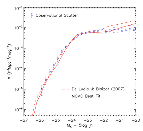
The comparison between the $K$-band luminosity function from the original DLB07 model (using the published parameter values) with the observations is shown in Fig.1. The original model already shows good agreement with the combined data except for the faint end, over predicting the number of dwarfs galaxies with magnitudes fainter than $K\approx-22$.

To compute the likelihood of the model for the $K$-band luminosity function we use the chi-square probability function where

$$\chi^{2}=\sum_{i}\frac{\left(N_{i}-n_{i}\right)^{2}}{\sigma_{i}^{2}+n_{i}}$$ (11)

is summed over the observational bin range plotted in Fig.1, and $N_{i}$ and $n_{i}$ represent the number of observational and simulated galaxies in each bin, respectively.

Figure 2: Correlations between the 6 parameters analysed in our study only constrained by the $\chi^{2}$ test on the $K$-band luminosity function. For the values of the parameters plotted in log space, the solid contours represent the 68% and 95% preferred regions from the MCMC (the posterior distribution) and the colours the maximum likelihood value sampled in each bin (the profile distribution). The colour scale is normalized by the maximum likelihood value of 0.87. White regions in the plot represent regions either with very low likelihood, less than 0.1 per cent of the peak, or regions that have not been visited by the MCMC chain.

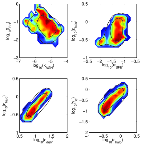
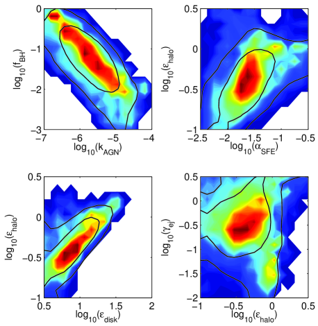
In Fig.2 we plot the 1$\sigma$ and 2$\sigma$ preferred values from the MCMC (solid lines) and the maximum likelihood value sampled in each bin (colour contours), for the subset of the original parameters (with values plotted in log space) constrained only by the observational $K$-band luminosity function.

In interpreting this and future plots, one should bear in mind that the contours follow the MCMC sampling in parameter space, which should trace out the relative likelihoods of different regions (the posterior distribution). The colours represent the maximum likelihood projected along all the hidden dimensions in the plot (profile distribution). Usually, as in this case, the two match fairly well. The exceptions arise when there is a high-likelihood region that only occupies a small volume of parameter space.

The two lower panels of Fig.2 show that the three parameters controlling the SN feedback are all positively correlated with each other, in a way that allows us to learn how the $K$-band luminosity function constrains the feedback model. To do this we rewrite equation 4 as

$${\Delta m_{\rm ejected}\over\Delta m_{\star}}=\epsilon_{\rm halo}\,\frac{V_{\rm SN}^{2}}{V_{\rm vir}^{2}}\,\left(1-{\epsilon_{\rm disk}\over\epsilon_{\rm halo}}\,\frac{V_{\rm vir}^{2}}{V_{\rm SN}^{2}}\right),$$ (12)

from which we see that the amount of ejected gas per unit mass of star formation drops to zero for halos with virial speed greater than

$$V_{\rm vir,0}=\left(\epsilon_{\rm halo}\over\epsilon_{\rm disk}\right)^{1\over 2}\,V_{\rm SN}.$$ (13)

In our analysis this cutoff is represented by the line of maximum likelihood in the lower left panel of Figure 2 and corresponds to $v_{\rm vir}\approx 140$ km s^-1, which translates into $M_{\rm star}\approx 10^{10.5}M_{\odot}$ and $M_{K}\approx-23$. This cutoff virial velocity is lower than in DLB07, which means that our SN feedback stops being effective at fainter magnitudes, allowing more stars to form in $L_{\star}$ galaxies. Since we need to assume a stronger SN feedback to decrease the faint end of the luminosity function, this is the only way to assure that enough stars will still form in brighter galaxies.

For a given value of $V_{\rm vir,0}$ the amount of ejected gas is proportional to $\epsilon_{\rm halo}$, with the maximum likelihood solutions showing a linear relation $\gamma_{\rm ej}\propto\epsilon_{\rm halo}$. This corresponds to a roughly constant amount of gas being held in the external reservoir: in a steady state the external gas content is proportional to the ratio of the influx and outflux rates. Our regions of high likelihood represent a considerably higher amount of gas being in the external reservoir than in DLB07 with a corresponding reduction in star formation in faint galaxies.

The value of $\epsilon_{\rm disk}$, controlling the reheating of cold to hot gas, has a minor impact except as a way of controlling the critical magnitude limit above which feedback is ineffective. Presumably cooling times are so short in galaxies below the magnitude limit that any gas that is reheated will quickly cool down again. One might have expected that it could be used to control the stellar mass fraction in large galaxies where the cooling time is relatively long, however this does not seem to be the case.

The AGN feedback parameters, shown in the top-left panel of Figure 2, have a broader acceptable region but also show a high-likelihood spine that runs diagonally down from top-left to bottom right. This can be explained by combining equations 6, 7 and 8 to obtain the mechanical heating rate produced by this process,

$$L_{\rm BH}\propto f_{\rm BH}\,k_{\rm AGN}\,m_{\rm cold}\,f_{\rm hot}.$$ (14)

Thus, for given cold and hot gas fractions in the galaxies, the line represents a single heating rate. This degeneracy is broken if the BH masses are used as a constraint (section 4.4), since their growth is mainly dominated by the quasar mode.

The maximum likelihood channels described above all have star-formation efficiencies of $\epsilon_{\rm SF}\approx 0.04$, similar to that of DLB07. This reinforces the conclusion that the SN and AGN feedback parameters act to maintain a constant mass of cold gas available for star-formation.

Apart from the main band discussed above, the two upper panels in Figure 2 show alternative regions of acceptable likelihood. These have lower star-formation efficiencies, requiring a greater mass of cold gas. This, in turn, leads to a smaller product of $f_{\rm BH}$ and $k_{\rm AGN}$. We do not dwell on these solutions here as they seem to be ruled out by other observations: in particular they result in excessive BH-bulge mass ratios.

4.3 The Colour-Stellar Mass Relation

The star formation rate is another essential quantity in characterising the galaxy population. Although this property can be directly extracted from the models, it is not easily comparable with observations. While in the models, the mass transformed into stars at each time step is computed, only indirect observational estimators are available.

Galaxy colours are one such indirect measure of the recent star-formation history of galaxies, with a clear bimodality between an old, passively evolving red population, and a young star forming blue sequence (e.g. Kauffmann et al., 2003; Brinchmann et al., 2004; Baldry et al., 2004).

Figure 3: Comparison between model and observational colours. The upper panel shows the DLB07 B-V colour-stellar mass relation, with the solid line representing the empirical division between populations in the model. On the bottom panel the fraction of red galaxies as a function of stellar mass from DLB07 (red open circles) and our best fit model (red filled circles) is compared with observations from Baldry et al. (2004) (filled blue squares).

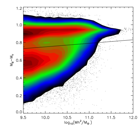
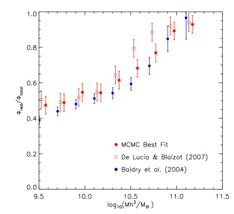
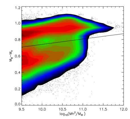
The top panel of Fig. 3 shows the colour-magnitude relation for the DLB07 model. Although it has some problems in correctly predicting the slope and fraction of each population in some mass ranges (see Baldry et al., 2006; Weinmann et al., 2006), it clearly reproduces the bimodality.

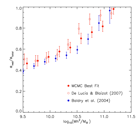
To test the correctness of model colours, we divide the galaxies into the two populations using the selection criteria in Weinmann et al. (2006), $(g-r)=0.7-0.032\,(M_{r}-5\log h+16.5)$, converted into a cut on the colour-stellar mass relation at redshift zero, $(B-V)=0.065\,\log({\rm M}_{\star}h^{2}/\hbox{$\rm\,M_{\odot}$})+0.09$, and shown as the solid line in the upper panel of Fig. 3. The conversion from the $g-r$ to the $B-V$ colour was done following Fukugita et al. (1996), $g-r=1.05(B-V)-0.23$. The fraction of red galaxies for different mass bins is then compared with observations from Baldry et al. (2004) as shown in the lower panel. The observational masses based on the ’diet’ Salpeter IMF (Bell et al., 2003) were reduced by 0.15 dex to agree with the IMF assumed in our semi-analytic model (Chabrier, 2003). The fact that a different blue band was used in the observational colour cut ($u-r$ instead of our converted $g-r$) could potentially lead to discrepancies in the number of objects identified in each population if the two gaussian distributions defining each population significantly overlap. However, as Fig. 3 shows, there is a clear division between red and blue galaxies in the $B-V$ CM diagram for model galaxies. In this way any small differences in the number of red galaxies caused by the different colour cut used, should be well within the 0.05 error assumed for the model fraction.

Following Croton et al. (2006) we take the resolution limit for model colours to be at a stellar mass of approximately $10^{9.5}\,h^{-2}\,M_{\odot}$, above which the model reproduces the red fraction reasonably well, with some minor excess for galaxies above $L_{\star}$.

The agreement between model and observational colours is calculated using a maximum likelihood method with a constant value for the errors in the model ($\sigma_{model}=0.05$) given by the variation in the fraction of red galaxies in a sample of 20 sub-volumes of the Millennium Simulation, similar to the one used in our analysis.

We assume that both model and observational values are Gaussian distributed around the true fraction $F$, with a likelihood

$$\mathcal{L}_{(\rm Colour)}=\exp\left\{-\frac{\left(f_{\rm model}-F\right)^{2}}{2\sigma_{\rm model}^{2}}-\frac{\left(f_{\rm obs}-F\right)^{2}}{2\sigma_{\rm obs}^{2}}\right\}$$ (15)

that has a maximum value

$$\mathcal{L}_{(\rm Colour)}=\exp\left\{-\frac{\left(f_{\rm model}-f_{\rm obs}\right)^{2}}{2(\sigma_{\rm model}^{2}+\sigma_{\rm obs}^{2})}\right\}.$$ (16)

Figure 4: As for Figure 2, but constrained only by the maximum likelihood test on the fraction of red galaxies. The colour scale is normalized by the maximum likelihood value of 0.89.

The DLB07 model, tuned to reproduce a different set of observational colours (the red and blue luminosity functions from 2DFGRS), correctly predicts the fraction of red galaxies at low and high masses but makes the transition from moderate to high red fractions at a stellar mass which is too low.

In Fig 4 we plot the allowed regions in likelihood and posterior space. Perhaps surprisingly, the colour constraint picks out a similar relationship between $\epsilon_{\rm halo}$ and $\epsilon_{\rm disk}$ as does the $K$-band. This is because it also requires a cessation of SN heating in galaxies with virial speeds above 140 km s^-1 which would otherwise have an excessive red fraction.

The constraint again requires a constant mechanical heating from AGN feedback (as shown by the line of maximum likelihood in the upper-left panel of the figure) which is responsible for the elimination of blue galaxies at high masses. The line of highest likelihood lies slightly below that seen for the $K$-band constraint. Along with this, the upper-right panel of the figure shows a preference for a slightly lower star-formation efficiency. However, in each case there is an acceptable region where the allowed parameter spaces overlap. This changes when we move to our third constraint.

4.4 The Black Hole-Bulge Mass Relation

We have seen in the previous section that the power of the radio-mode AGN feedback depends upon the product of the quasar and radio-mode growth factors. However, the mass growth of the BHs is dominated by the quasar mode alone. We can therefore use the BH-bulge mass relation to break this degeneracy.

If we require semi-analytic galaxies to be constrained solely by this relation, then the other parameters in the model will be free to shift into implausible values allowing any point in parameter space to have a reasonable likelihood. For this reason, we require model galaxies to follow both the BH-bulge mass relation and the $K$-band luminosity function of bright galaxies (i.e. the host galaxies of these BHs).

The BH and bulge masses for the original model are plotted in Fig. 5 and compared with local observations from Häring & Rix (2004). The model galaxies fall on top of the observational best fit (given by the blue line), with the scatter in the relation also reproduced.

Figure 5: The BH-bulge mass relation for DLB07 (contours and dots) is compared with local observational data from Häring & Rix (2004) (blue crosses). The best fit to the observational data points is given by the blue line running from bottom-left to top-right, while the two black lines perpendicular to this relation divide galaxies into the two mass bins used to compute the likelihood.

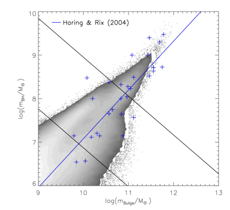
In order to test the semi-analytic results against observations, we divide the data into two bins (perpendicular to the observational best fit), represented by the solid black lines on Fig. 5, $15.2<m_{\rm BH}+0.90\,m_{\rm Bulge}\leq 17.75$ and $17.75<m_{\rm BH}+0.90\,m_{\rm Bulge}$, and for each of the bins we compute the binomial probability for the observed distribution of mass ratios above and below the best-fit line, given the fractional distribution from the model galaxies:

$$\mathcal{L}_{(\mathrm{BH-Bulge})}=\left\{\begin{array}[]{ll}2I_{p}(k,n-k+1),&I_{p}\leq 0.5\\ 2(1-I_{p}(k,n-k+1)),&I_{p}>0.5\end{array}\right.$$ (17)

where $k$ is the number of observed galaxies above the best fit in each bin, $n$ the total number of observed galaxies in the same bin, and $p$ is the equivalent fraction, $k/n$, for the model galaxies in the bin. $I_{p}(a,b)$ is the incomplete beta function as defined in Press et al. (2007). The two formulae are required since we need to exclude both extremes of the distribution, corresponding to an excess of points both above and bellow the best-fit line.

In Fig. 6 we plot the posterior and profile likelihood distributions of the parameters constrained only by this binomial test and the $K$-band luminosity function of galaxies brighter than $M_{k}=-23$.

Figure 6: As for Figure 2, but constrained only by the binomial test on the BH-bulge mass relation and by the $K$-band luminosity function of galaxies above $M_{k}=-23$. The colour scale is normalized by the maximum likelihood value of 0.86.

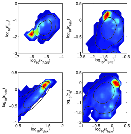
It is immediately apparent that the region of high likelihood is much smaller for this test than for the first two constraints. Moreover, this region corresponds to high values for the SN feedback parameters, combined with a low AGN feedback efficiency. As such, it is incompatible with the acceptable regions in those previous tests.

However, there is a lower-likelihood, but still acceptable (likelihood $>0.1$) region that extends towards lower SN and higher AGN parameters. As the MCMC contours show, this occupies a much larger volume of parameter space than the high-likelihood peak (and so, in a Bayesian sense, the true solution is more likely to be found in the former than the latter).

Looking at the upper-left panel in the figure, we can see that the acceptable region runs from bottom-left to top-right, perpendicular to the lines seen in the previous two tests. The BH-bulge mass ratio thus breaks the degeneracy in the AGN parameters.

5 Combined observational constraints

Figure 7: As for Figure 2, but constrained by all three observational properties: the $K$-band luminosity function, the fraction of red galaxies, and the BH-bulge mass relation. The colour scale is normalized by the maximum likelihood value of 0.037.

Figure 8: Likelihood distributions for the 6 parameters studied. The solid lines represent the maximum likelihood in each bin marginalised over the other dimensions in parameter space.

The likelihood of the model for a given point in parameter space is computed by taking the product of the three independent observational constraints described in the previous sections.

$$\pi(x_{i})=\mathcal{L}_{(\rm K-Band)}\times\mathcal{L}_{(\rm Colour)}\times\mathcal{L}_{(\mathrm{BH-Bulge})}$$ (18)

This quantity is calculated at each MCMC step and used to derive the acceptance probability (equation 10). We run our sampling over approximately 30 000 steps, excluding an initial burn-in to assure the independence of the final results from the starting point of the chain. The output is then analysed using getdist, part of the COSMOMC software package (Lewis & Bridle, 2002). As for the individual constraints, the code is adapted to produce 1d and 2d maximum likelihood (profile) and MCMC marginalised (posterior) distributions, best values and confidence limits for the parameters, convergence statistics for the chain and correlation statistics for each parameter.

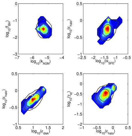
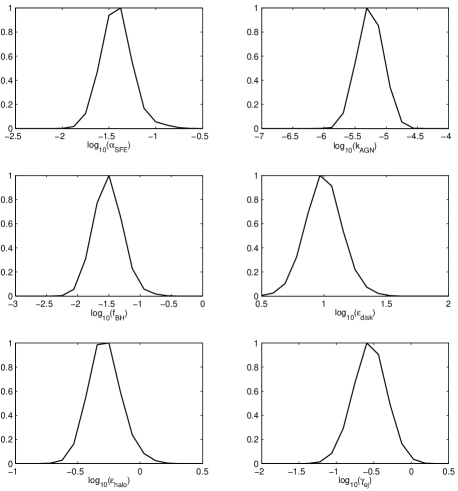
Although, in our sampling we do not impose rigid limits on the parameter range, Figure 7 shows that the preferred regions are well-constrained. Figure 8 shows the profile distribution for each parameter, marginalised over all others. Unfortunately, the maximum likelihood is just 0.037, thus the best-fit solution is incompatible with the three combined observations at the 2-$\sigma$ level.

The principal cause of the low likelihood is an incompatibility between the BH-bulge mass constraint and the $K$-band and $B-V$ colours. As discussed in section 6, this might be caused by observational uncertainties in the black hole and bulge masses or might reflect a deficiency in the black hole growth model, which is still very simplistic. Nevertheless, observational uncertainties, principally that associated with stellar population synthesis modelling, make it premature to conclude that the DLB07 formalism is ruled out.

5.1 Best Fit Parameters and Confidence Limits

Table 2: Statistics from the MCMC parameter estimation for the 6 parameters selected from the original model. The best fit and confidence limits (derived from the colour contours in Fig. 7) are compared with the published values from DLB07.

	DLB07	Mean	lower (2$\sigma$ limit)	lower (1$\sigma$ limit)	upper (1$\sigma$ limit)	upper (2$\sigma$ limit)
$\alpha_{SF}$ (SFE)	0.03	0.039	0.020	0.020	0.11	0.13
$k_{AGN}$ (AGN Radio)	$7.5\times 10^{-6}$	$5.0\times 10^{-6}$	$2.4\times 10^{-6}$	$2.4\times 10^{-6}$	$9.7\times 10^{-6}$	$1.1\times 10^{-5}$
$f_{BH}$ (AGN Quasar)	0.03	0.032	0.014	0.014	0.103	0.115
$\epsilon_{disk}$ (SN Reheating)	3.5	10.28	4.43	4.52	24.37	24.37
$\epsilon_{halo}$ (SN Ejection)	0.35	0.53	0.26	0.26	1.17	1.17
$\gamma_{ej}$ (SN Reincorporation)	0.5	0.42	0.08	0.08	0.73	0.79

The best fit and confidence limits for the 6 free parameters, together with the published values from DLB07 are shown in table 2. All the parameter values in the original model fall within our 2$\sigma$ regions except for the SN disk reheating efficiency, which we require to be larger than before.

Both the star formation efficiency and the AGN quasar mode parameters from DLB07 closely match our best fit values, while our AGN radio mode efficiency is slightly lower than before.

For the SN feedback parameters, the original halo ejection efficiency, $\epsilon_{\rm halo}$ is below our best fit, whereas the original gas reincorporation efficiency, $\gamma_{\rm ej}$, is slightly higher. This combination acts so as to produce a higher fraction of gas trapped in the external reservoir with the new parameters, and hence a smaller mass of cold gas available for star-formation in dwarf galaxies.

The DLB07 SN reheating efficiency $\epsilon_{disk}$, is considerably lower than our best-fit. As discussed earlier, the main effect of this is to raise the ratio $\epsilon_{\rm disk}/\epsilon_{\rm halo}$ with the new parameters and hence, from equation 13, to lower the critical virial speed above which feedback is ineffective.

5.2 Galaxy Properties in our Best Fit Model

The MCMC parameter estimation was carried out using only one data-file representing 1/512 of the Millennium volume. In this section we present results using our best-fit parameters in the full volume.

5.2.1 Galaxy Luminosity Functions

Figure 9: Comparison of the predicted $K$-band (left panel) and $b_{\rm J}$-band (right panel) luminosity functions at $z=0$ from DLB07 (dashed red line) and our best fit model (solid red line). On the left panel, the data points represent the observations used to constrain the luminosities of galaxies in our MCMC parameters estimation (Cole et al., 2001; Bell et al., 2003; Jones et al., 2006). On the right panel, the $b_{\rm J}$-band luminosity function is compared with observations from 2DFGRS (green filled squares) and 6DFGS (blue open circles), respectively Norberg et al. (2002) and Jones et al. (2006).

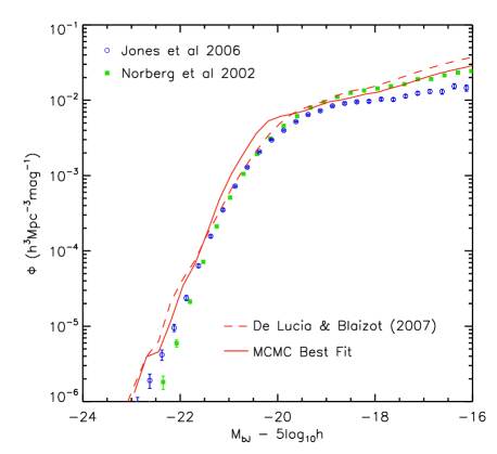
The requirement that star formation be inefficient in low-mass galaxies is a common problem to both sets of semi-analytic models built upon the Millennium Simulation. There is an apparent excess of dwarf galaxies that can be seen in the $K$-band luminosity function in both Croton et al. (2006) and Bower et al. (2006).

In the left panel of Fig. 9 the $K$-band luminosity functions from DLB07 and our best-fit model are plotted against the observational data set used to constrain the sampling. As discussed in section 4.2, to get a good agreement with observations, the model needs to form considerably fewer stars in low mass galaxies. This is achieved by reducing the amount of cold gas available for star-formation by increasing the SN heating efficiency and decreasing the amount of gas reincorporated at each time step. To assure that enough $L_{\star}$ galaxies are produced, the virial velocity cutoff above which SN feedback is ineffective is lowered, by raising $\epsilon_{\rm disk}$ relative to $\epsilon_{\rm halo}$ (equation 13).

In the right panel of Fig.9, the best-fit model seems to show poorer agreement with the $b_{\rm J}$-band than the original DLB07. The new fit does reproduce the number-density of dwarf galaxies accurately, but shows a large excess around $L_{\star}$. This is partly a reflection of the excess seen in the $K$-band in the same region, but has a large magnitude. Given the good match to the colour fraction, this seems surprising and points to inconsistencies and/or uncertainties in the conversion of mass to luminosity via stellar population synthesis (see section 5.3).

5.2.2 Galaxy Colours

In Fig. 10 we show the predicted galaxy colours in our best fit model, the $B$-$V$ colour-stellar mass relation on the top panel and the fraction of red over the total number of galaxies as a function of stellar mass in the bottom panel. Our best fit correctly reproduces the fraction of red galaxies by slightly increasing the number of blue galaxies around $L_{\star}$ compared to DLB07.

The colour-stellar mass relation also shows improvements, keeping the bimodality between the red and the blue galaxies, but increasing the slope of each population as suggested by observations. Nevertheless, near the lower-mass limit we impose in our study a population of red dwarfs starts to emerge, representing the highest number density peak in the red population. This is in disagreement with observations, where the majority of the red galaxies are massive, and the dwarfs are predominately blue. We address this problem, and explore possible solutions in section 6.

Figure 10: The top panel shows the $B$-$V$ colour-stellar mass relation for the galaxies in our best fit model. The solid line represents the division between the red and blue populations in Weinmann et al. (2006). The predicted fraction of red galaxies as a function of stellar mass is showed in the bottom panel. The original DLB07 model (open red circles) is compared with our best fit model (filled red circles) and observational data from Baldry et al. (2004) (filled blue squares).

5.2.3 The Black Hole-Bulge Mass Relation

The best-fit BH-bulge mass relation is almost unchanged from that shown in Figure 5 and so we do not repeat it here. There is enough freedom in the model to allow the AGN parameters to adjust themselves to recover the correct BH masses, despite the differences in the SN parameters between DLB07 and out best fit.

5.3 The Galaxy Stellar Mass Function

Figure 11: Comparison for the predicted stellar mass function at z=0 from DLB07 (dashed red line) and our best-fit model (solid red line) with observations from Baldry et al. (2008) (blue open circles) and Bell et al. (2003)(green filled squares).

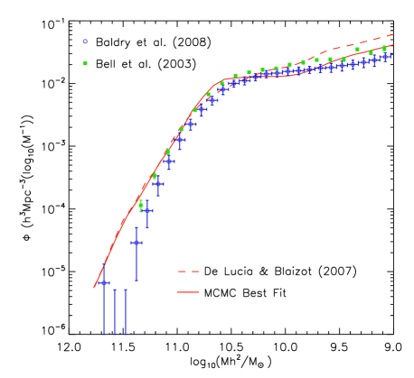
As discussed in section 4.2, the stellar mass function is one of the most fundamental properties of a galaxy population, but it is difficult to derive accurately from observations. In Fig. 11 we show how our best-fit model and DLB07 masses compare with observationally-derived stellar mass functions from Bell et al. (2003) and Baldry et al. (2008). The latter is one of the most robust mass derivations, using the New York University Value-Added Galaxy Catalogue that combines 4 different methods for determining galaxy masses from SDSS data. The error bars in the figure span the maximum and minimum mass estimates from that analysis.

After all the data sets are converted into the same IMF (that of Chabrier, 2003), the comparison between our best-fit model and the masses derived from Bell et al. (2003) in Fig. 11 shows the same behaviour as the $K$-band luminosity function. With our more effective supernova feedback the excess of dwarf galaxies largely disappears, but there is a slight excess of $L\star$ galaxies. Small differences might arise when comparing both the $k$-band and stellar mass functions from the model and a specific observational data set, even though similar stellar population synthesis models were used. This is because, to convert stellar mass into luminosity, one should have knowledge about the age and metallicity of the galaxy stellar population. These quantities are directly available in the model, but in observations they are difficult to derive and are subject to large uncertainties.

Also shown in Fig. 11 is a comparison of the predicted masses with data from Baldry et al. (2008). A systematic difference between the model and the data is evident, with the former predicting a much larger number of galaxies on and above $L\star$. While the horizontal error bars plotted in Fig. 11 for Baldry et al. (2008) reflect only the bin size, the authors refer to differences as large as 0.15 dex in mass estimates from the different methods. Another recent work (Conroy et al., 2008) points to even larger errors of up to 0.3 dex that may result from imprecise modelling of key phases of stellar evolution. If these uncertainties lead to the observationally-derived masses of large galaxies being underestimated by about 0.15 dex, then our best fit and observations from Baldry et al. (2008) would be in extremely good agreement throughout the whole mass range.

The differences between data sets highlight the need for caution when galaxy formation models are compared with observations. In principle one should expect the properties and allowed parameter ranges to change if either the stellar population synthesis or the dust model need to be readjusted. In this paper we have chosen to fix these so as to focus our study on the parameters controlling the most basic properties of the semi-analytic model: star formation and feedback.

6 Discussion and Conclusions

Since they were introduced as a new technique to understand galaxy formation (White & Rees, 1978; White & Frenk, 1991; Lacey & Silk, 1991; Cole, 1991), semi-analytic models have always lacked a proper statistical analysis of the allowed range of their free parameters and a consistent way to test the goodness of the fits produced.

To overcome this weakness we have implemented a Monte Carlo Markov Chain parameter estimation technique into the De Lucia & Blaizot (2007) semi-analytic model, to obtain the best values and confidence limits for the 6 free parameters in the model responsible for shaping the stellar mass function and for the colours of galaxies. Comparing the model with three different observational constraints separately: the combined $K$-band luminosity function from Cole et al. (2001); Bell et al. (2003); Jones et al. (2006), galaxy colours from Baldry et al. (2004) and the BH-bulge mass relation from Häring & Rix (2004), we are able to identify which particular parameters (and hence which galaxy formation processes) are responsible for each individual property and which show correlations and degeneracies.

Combining the three observational tests, we are able to fully constrain the model parameters, obtaining a best fit and confidence limits within the very limited region of acceptable likelihood. Our best model is given by: $\alpha_{SF}=0.039_{-0.019}^{+0.091}$, $k_{AGN}=(5.0_{-2.6}^{+6.0})\times 10^{-6}$, $f_{BH}=0.032_{-0.018}^{+0.083}$, $\epsilon_{disk}=10.28_{-5.85}^{+14.09}$, $\epsilon_{halo}=0.53_{-0.27}^{+0.64}$ and $\gamma_{ej}=0.42_{-0.34}^{+0.37}$). As shown in table 2, all the parameters in the original model, except the supernova reheating efficiency fall within our 2-$\sigma$ confidence limits. Our best fit maintains the values for the star formation efficiency and for the AGN quasar mode parameters, while increasing the SN gas reheating and ejection and decreasing the AGN radio mode and gas reincorporation efficiencies. For our preferred set of parameters the model has a likelihood of $\pi(x_{i})={L}_{\rm(Mass)}\times{L}_{\rm(Colour)}\times{L}_{(\mathrm{BH-Bulge})}=0.037$. This value means that the best-fit solution is incompatible with the three combined observations at the 2-$\sigma$ level.

In this paper, we have used the Millennium Simulation which adopts a $\Lambda$CDM cosmology. It is possible that the Universe may be better described by an alternative cosmology with fewer low-mass halos. However, our purpose here is to try to find an astrophysical solution that is compatible with $\Lambda$CDM.

As discussed in previous chapters, observational uncertainties, principally that associated with stellar population synthesis and dust modelling, make it premature to conclude that the DLB07 formalism is ruled out: shifting the observed black-hole/bulge mass ratio by 0.15 dex raises the best-fit likelihood to 0.07, which is marginally acceptable. Nevertheless, the apparent incompatibility between the black hole-bulge mass relation and the other constraints indicates that the black hole growth treatment in the model might be too simplistic, in particular by assuming that there is no feedback from the quasar mode, when it seems to be required to reproduce the X-ray luminosity function of halos (Bower et al., 2008; Short & Thomas, 2008). As discussed below, some additional recipes might also need to be included for the model to better reproduce observational luminosities and colours, which could in principle increase the likelihood of the best fit model.

We produce a $K$-band luminosity function for our best parameter values that improves the agreement with observations at the low-luminosity end. This is achieved by taking a higher heating efficiency from SN and a lower reincorporation rate of gas ejected from the halo. This reduces the amount of cold gas available to form stars, avoiding the excess of faint galaxies in the original recipe. More effective SN feedback has been proposed in the past. For example, Bertone et al. (2007) studied a wind model that improved the number density of dwarfs for both the mass and luminosity function while improving the distribution of metals. However, the high value of ejection that is required by our model seems to be unrealistic when compared with observations (Martin, 1999). This indicates that additional processes such as disruption of satellites through tidal effects might need to be included (Bullock et al., 2001; Taylor & Babul, 2001; Benson et al., 2002; Monaco et al., 2006; Weinmann et al., 2006; Murante et al., 2007; Henriques et al., 2008; Somerville et al., 2008).

For both the luminosity-function and colour constraints, the SN reheating and ejection parameters are strongly correlated, which we interpret as an upper virial velocity limit of 140 km s^-1 for galaxies that can eject mass via SN heating. Since we need to assume a stronger SN feedback to decrease the faint end of the $K$-band luminosity function, this relatively low value assures that our SN feedback stops being effective for galaxies with masses above $M_{\star}\approx 10^{10.5}M_{\odot}$. This is the only way to ensure that enough stars will form in brighter galaxies, and also produces more blue galaxies around $L_{\star}$ than the original DLB07 parameters.

Significant correlations exist between the three parameters governing SN feedback , $\epsilon_{\rm disk}$, $\epsilon_{\rm halo}$ & $\gamma_{\rm ej}$, even in the combined analysis. This suggests that the model could be rewritten with one or two fewer free parameters. However this degeneracy could in principle be broken if the metallicity of gas and stars were to be considered.

The model with the original DLB07 parameters correctly predicts the bimodality in the colour-stellar mass relation, however, it has difficulties in matching the exact number of the blue and red sequence galaxies. Our best-fit model correctly predicts the relative fraction of galaxies in each colour population, however the early cutoff on SN feedback leads to an excess of galaxies with masses between $10^{10.5}$ and $10^{11.0}$ $\rm\,M_{\odot}$. Furthermore, as the original model, it shows a large population of small red galaxies in the $B-V$ colour-stellar mass plot in contradiction with observations.

The problems with low-mass galaxy colours in semi-analytic models have been identified in the past, particularly the excess of red dwarfs (Croton et al., 2006; Baldry et al., 2006). Possible solutions might include the delayed stripping of gas from satellites after their dark matter halo is disrupted (allowing them to cool gas, form stars and stay blue for longer Font et al. 2008). Or again, tidal disruption of dwarfs, which would affect mostly red, satellite galaxies. This would move them to even lower masses, below $10^{9.0}M_{\odot}$ (where an upturn in the stellar mass function is seen) and produce intra-cluster light (Weinmann et al., 2006; Henriques et al., 2008; Somerville et al., 2008).

The purpose of this paper is to show that MCMC parameter estimation techniques, adapted from those used in cosmology, can be used to map out likelihood contours in the parameter space of semi-analytic models of galaxy formation. For this particular analysis we chose the formalism of De Lucia & Blaizot (2007), but the same method could equally be applied to other models.

In the future, we would like to extend the method to undertake model selection, providing an objective measure of the relative value of models with different numbers of free parameters.

References

- Baldry et al. (2006) Baldry I. K., Balogh M. L., Bower R. G., Glazebrook K., Nichol R. C., Bamford S. P., Budavari T., 2006, MNRAS, 373, 469
- Baldry et al. (2004) Baldry I. K., Glazebrook K., Brinkmann J., Ivezić Ž., Lupton R. H., Nichol R. C., Szalay A. S., 2004, ApJ, 600, 681
- Baldry et al. (2008) Baldry I. K., Glazebrook K., Driver S. P., 2008, MNRAS, 388, 945
- Bell et al. (2003) Bell E. F., McIntosh D. H., Katz N., Weinberg M. D., 2003, ApJ Supp., 149, 289
- Benson et al. (2003) Benson A. J., Bower R. G., Frenk C. S., Lacey C. G., Baugh C. M., Cole S., 2003, ApJ, 599, 38
- Benson et al. (2002) Benson A. J., Lacey C. G., Baugh C. M., Cole S., Frenk C. S., 2002, MNRAS, 333, 156
- Bertone et al. (2007) Bertone S., De Lucia G., Thomas P. A., 2007, MNRAS
- Bower et al. (2006) Bower R. G., Benson A. J., Malbon R., Helly J. C., Frenk C. S., Baugh C. M., Cole S., Lacey C. G., 2006, MNRAS, 370, 645
- Bower et al. (2008) Bower R. G., McCarthy I. G., Benson A. J., 2008, MNRAS
- Brinchmann et al. (2004) Brinchmann J., Charlot S., White S. D. M., Tremonti C., Kauffmann G., Heckman T., Brinkmann J., 2004, MNRAS, 351, 1151
- Bullock et al. (2001) Bullock J. S., Kravtsov A. V., Weinberg D. H., 2001, ApJ, 548, 33
- Cattaneo et al. (2006) Cattaneo A., Dekel A., Devriendt J., Guiderdoni B., Blaizot J., 2006, MNRAS, 370, 1651
- Chabrier (2003) Chabrier G., 2003, PASP, 115, 763
- Cole (1991) Cole S., 1991, ApJ, 367, 45
- Cole et al. (1994) Cole S., Aragon-Salamanca A., Frenk C. S., Navarro J. F., Zepf S. E., 1994, MNRAS, 271, 781
- Cole et al. (2000) Cole S., Lacey C. G., Baugh C. M., Frenk C. S., 2000, MNRAS, 319, 168
- Cole et al. (2001) Cole S., Norberg P., Baugh C. M., et al., 2001, MNRAS, 326, 255
- Conroy et al. (2008) Conroy C., Gunn J. E., White M., 2008, ArXiv e-prints
- Croton et al. (2006) Croton D. J., Springel V., White S. D. M., De Lucia G., Frenk C. S., Gao L., Jenkins A., Kauffmann G., Navarro J. F., Yoshida N., 2006, MNRAS, 365, 11
- Daigne et al. (2004) Daigne F., Olive K. A., Vangioni-Flam E., Silk J., Audouze J., 2004, ApJ, 617, 693
- De Lucia & Blaizot (2007) De Lucia G., Blaizot J., 2007, MNRAS, 375, 2
- De Lucia et al. (2004) De Lucia G., Kauffmann G., White S. D. M., 2004, MNRAS, 349, 1101
- Font et al. (2008) Font A. S., Bower R. G., McCarthy I. G., Benson A. J., Frenk C. S., Helly J. C., Lacey C. G., Baugh C. M., Cole S., 2008, arXiv:astro-ph/0807.0001
- Fukugita et al. (1996) Fukugita M., Ichikawa T., Gunn J. E., Doi M., Shimasaku K., Schneider D. P., 1996, AJ, 111, 1748
- Granato et al. (2004) Granato G. L., De Zotti G., Silva L., Bressan A., Danese L., 2004, ApJ, 600, 580
- Häring & Rix (2004) Häring N., Rix H.-W., 2004, ApJ, 604, L89
- Hastings (1970) Hastings W. K., 1970, Biometrika, 57, 97
- Hatton et al. (2003) Hatton S., Devriendt J. E. G., Ninin S., Bouchet F. R., Guiderdoni B., Vibert D., 2003, MNRAS, 343, 75
- Henriques et al. (2008) Henriques B. M., Bertone S., Thomas P. A., 2008, MNRAS, 383, 1649
- Jones et al. (2006) Jones D. H., Peterson B. A., Colless M., Saunders W., 2006, MNRAS, 369, 25
- Kampakoglou et al. (2008) Kampakoglou M., Trotta R., Silk J., 2008, MNRAS, 384, 1414
- Kang et al. (2005) Kang X., Jing Y. P., Mo H. J., Börner G., 2005, ApJ, 631, 21
- Kauffmann et al. (1999) Kauffmann G., Colberg J., Diaferio A., White S., 1999, MNRAS, 303, 188
- Kauffmann & Haehnelt (2000) Kauffmann G., Haehnelt M., 2000, MNRAS, 311, 576
- Kauffmann et al. (2003) Kauffmann G., Heckman T. M., White S. D. M., et al., 2003, MNRAS, 341, 33
- Kauffmann et al. (1993) Kauffmann G., White S. D. M., Guiderdoni B., 1993, MNRAS, 264, 201
- Kennicutt (1998) Kennicutt Jr. R. C., 1998, ApJ, 498, 541
- Kravtsov et al. (2004) Kravtsov A. V., Gnedin O. Y., Klypin A. A., 2004, ApJ, 609, 482
- Lacey et al. (1993) Lacey C., Guiderdoni B., Rocca-Volmerange B., Silk J., 1993, ApJ, 402, 15
- Lacey & Silk (1991) Lacey C., Silk J., 1991, ApJ, 381, 14
- Lewis & Bridle (2002) Lewis A., Bridle S., 2002, Phys. Rev., 66, 103511
- Martin (1996) Martin C. L., 1996, ApJ, 465, 680
- Martin (1999) Martin C. L., 1999, ApJ, 513, 156
- Menci et al. (2002) Menci N., Cavaliere A., Fontana A., Giallongo E., Poli F., 2002, ApJ, 575, 18
- Menci et al. (2006) Menci N., Fontana A., Giallongo E., Grazian A., Salimbeni S., 2006, ApJ, 647, 753
- Metropolis et al. (1953) Metropolis N., Rosenbluth A., Rosenbluth M., Teller A., Teller E., 1953, JCP, 21, 1087
- Monaco (2004) Monaco P., 2004, MNRAS, 352, 181
- Monaco et al. (2007) Monaco P., Fontanot F., Taffoni G., 2007, MNRAS, 375, 1189
- Monaco et al. (2006) Monaco P., Murante G., Borgani S., Fontanot F., 2006, ApJ, 652, L89
- Murante et al. (2007) Murante G., Giovalli M., Gerhard O., Arnaboldi M., Borgani S., Dolag K., 2007, MNRAS, 377, 2
- Norberg et al. (2002) Norberg P., Cole S., Baugh C. M., et al., 2002, MNRAS, 336, 907
- Press & Schechter (1974) Press W. H., Schechter P., 1974, ApJ, 187, 425
- Press et al. (2007) Press W. H., Teukolsky A. A., Vetterling W. T., Flannery B. P., 2007, Numerical Recipes, The Art of Scientific Computing - Third Edition. ambridge University Press
- Short & Thomas (2008) Short C. J., Thomas P. A., 2008, ArXiv e-prints
- Somerville et al. (2008) Somerville R. S., Hopkins P. F., Cox T. J., Robertson B. E., Hernquist L., 2008, MNRAS, 391, 481
- Somerville & Primack (1999) Somerville R. S., Primack J. R., 1999, MNRAS, 310, 1087
- Springel et al. (2005) Springel V., White S. D. M., Jenkins A., et al., 2005, Nat., 435, 629
- Springel et al. (2001) Springel V., White S. D. M., Tormen G., Kauffmann G., 2001, MNRAS, 328, 726
- Taylor & Babul (2001) Taylor J. E., Babul A., 2001, ApJ, 559, 716
- Trotta (2008) Trotta R., 2008, Contemporary Physics, 49, 71
- Weinmann et al. (2006) Weinmann S. M., Van Den Bosch F. C., Yang X., Mo H. J., 2006, MNRAS, 366, 2
- Weinmann et al. (2006) Weinmann S. M., Van Den Bosch F. C., Yang X., Mo H. J., Croton D. J., Moore B., 2006, MNRAS, 372, 1161
- White & Frenk (1991) White S. D. M., Frenk C. S., 1991, ApJ, 379, 52
- White & Rees (1978) White S. D. M., Rees M. J., 1978, MNRAS, 183, 341