On alpha stable distribution of wind driven water surface wave slope

Abstract

We propose a new formulation of the probability distribution function of wind driven water surface slope with an $\alpha$-stable distribution probability. The mathematical formulation of the probability distribution function is given under an integral formulation. Application to represent the probability of time slope data from laboratory experiments is carried out with satisfactory results. We compare also the $\alpha$-stable model of the water surface slopes with the Gram-Charlier development and the non-Gaussian model of Liu et alLiu . Discussions and conclusions are conducted on the basis of the data fit results and the model analysis comparison.

Keywords: Wind driven water surface wave slopes. Probability density function. Non-Gaussian distribution. Alpha-stable distribution.
During the last three decades, remote sensing of ocean surface has been extensively investigated to study physical processes on the sea surface and air sea interaction mechanism. One of the most important quantities on which depends the ocean remote sensing process is the surface wave slope probability distribution that is known to be non-Gausssian. In the past the general way to describe such probability distribution was to use an expansion technique of the Gaussian law known as Gram-Charlier series. In the present paper, we propose a new formulation of the surface wave slope using alpha stable probability distribution. Application to data from laboratory experiments and comparison of the alpha stable slope model with existing models are carried out. Our results show the potentiality of the alpha stable laws to describe the non-Gaussian variability of water surface wave slope.

I Introduction:

A knowledge of the sea surface slope distribution and its related statistical quantities is essential to study the sea surface using remote sensing processes. The use of radar backscatter to characterize the sea surface has been widely investigated experimentally and theoretically. At nearly normal radar beam incidence, the importance of the slope distribution is clearly exhibited by the simplest model of cross section radar backscatter based on geometrical optics approach formulated by ValenzuelaValenz as:

$$\sigma_{0}(\theta)=\pi sec^{4}\theta f(\zeta_{x},\zeta_{y})|R(0)|^{2}$$ (1)

where $\theta$ is the radar incidence angle, $|R(0)|^{2}$ is the Fresnel reflection coefficient for normal incidence and $f(\zeta_{x},\zeta_{y})$ is the probability distribution function (PDF) of the sea surface slope at specular point $(\zeta_{x},\zeta_{y})$. Determination of the surface slope distribution has been carried out in a large part with semi-empirical models derived from data observations. The commonly used approach for such purpose was the truncated Gram-Charlier series under the assumptions of the near-Gaussian case and the weakly nonlinear interaction proposed by Longuet-HigginsLonguet . The Gram-Charlier series was attempted to include two additional factors: the skewness and the peakedness that are respectively due to second and third order wave-wave interactions. Despite the multiple adaptations made on the Gram-Charlier model, it is now well-known that this approach fails to work in the range of large slope or large surface elevation. In other word, this model is not suitable to represent the reality when large events have higher occurrence. To improve the results from Gram-Charlier series, several works were made by different authors. Among the existing models, those of Liu et alLiu , differs by its formulation and its mathematical nature. Indeed, Liu model does not appeal to an expansion technique and is well suitable to represent extreme events. However, this model is originally a symmetrical law including the Gaussian probability and the Cauchy law as limit cases. Owing to the symmetry property, the Liu model is not able to reproduce the skewness effect. Liu extended empirically the model for this purpose.

In the present paper we propose to use the $\alpha$-stable law to describe the PDF of surface slope. The stable law depends on four parameters: the index of stability, the skewness, the scale and the location parameters that allow one to represent a probability law of random variations including asymmetry, peakedness and peak shift. Also, the $\alpha$-stable law includes as limit cases the Gaussian probability and the Cauchy law. Generally speaking, stable law belongs to the family of heavy tails probability laws that is especially well adapted to take in account the large events of random variations. Such strong random variations can be found in fields or laboratory observations of the water surface roughness (Onorato et alOno1 ).

Evidences from in situ and laboratory experiments of non-Gaussian heavy tails distribution of wind driven water surface waves and their slope may be found in many articles in the literature. The first argument on the non-Gaussian behavior of wind driven water surface waves and their slopes concerns the existence of asymmetry property of wind wavefield that can be quantified by higher order spectral analysis (Leykin et alLeykin ,Joelson et alJoelson ). Another hallmark of this non-Gaussian behavior is based on the power law observed in the spectrum of wind driven water surface waves. We cite here some works emphasizing this fact. Experiment observations was conducted by HuangHuang on time series of sea surface that suggest a random dynamic as a spectral power law associated to fractal description. Mellen and alMellen performed the study of random nonlinear dynamics of laboratory wind waves by the Lévy index and the co-dimension parameter that quantify the multifractal property of the water surface. As pointed out by Solow Solow , power law behaviour can arise from random distributions having heavy upper tail. A fundamental consequence is that random rough surfaces with slowly decaying power spectral density can have infinite slope variance (Warnick et alWarnick ). Such case of slope behavior is clearly beyond the Gaussianity assumption and is only reached by the family of heavy tail probability distribution model. The $\alpha$-stable law belongs to this class of model. Heavy tail distributions of wind driven water surface slope obtained from experiment observations can be found in different works (see for example Cox and Munk Cox1 , Lui et alLiu , Chapron et alChapron ).

Direct simulation methods such as a Monte-Carlo simulation based on nonlinear hydrodynamical model are able to reproduce pseudo-random samples that present similar aspects. Recently, Soriano et alSoriano studied the effect of this non-Gaussian character on the radar Doppler spectrum of the random surface at grazing angle and concluded on the importance of the non-Gaussian character. Despite these results and the fact that stable laws have been discovered several decades ago, there are only few applications concerning the $\alpha$-stable distribution of sea surface. In particular, we cite here the work of Guéringuerin on the scattering on random rough surface with $\alpha$-stable law in which he gave an extension of the expression (1) for the $\alpha$-stable surface roughness.

The present study, in our opinion, is the first attempt to apply the stable probability law on random water surface slope representation. The paper is organized as follow: in §2, we recall the main properties of the $\alpha$-stable law. In §3, the application of stable law to fit instantaneous slope of wind driven water surface is presented. The §4 is devoted to the comparison of the stable PDF with the Gram-Charlier model and the Liu model. In §5, we present our conclusions on the results of the study.

II Stable probability distribution

The stable laws were introduced by Paul Lévy L vy during his investigations of the behavior of the sums of independent identically distributed random variables. Then the theory on stable laws was developed by many authors and laid out in many books and articles. We recall here some basic results without proof. A stable distribution law is determined by four parameters: an index of stability $\alpha$, a location parameter $\mu$, a skewness parameter $\beta$ and a scale parameter $\gamma$. The most common formulation of such law is given by the characteristic function which represents the inverse Fourier transform of the probability distribution function. A random variable X is said to have a stable distribution (noted as $\mbox{X}\sim S_{\alpha}(\beta,\gamma,\mu)$) if its characteristic function satisfies

$$\Phi_{X}(t)=\mbox{exp}\left(i\mu t-\gamma^{\alpha}|t|^{\alpha}\left[1-i\beta\mbox{ sign}(t)\mbox{ W}(\alpha,t)\right]\right)$$ (2)

where

$$\mbox{W}(\alpha,t)=\left\{\begin{array}[]{rl}\mbox{ tan}(\frac{\pi\alpha}{2})&\mbox{if }\alpha\neq 1\\ -\frac{2}{\pi}\mbox{log }|t|&\mbox{if }\alpha=1\end{array}\right.$$

and

$$\mbox{sign}(t)=\left\{\begin{array}[]{rl}\mbox{1}&\mbox{if }t>0\\ \mbox{0}&\mbox{if }t=0\\ \mbox{-1}&\mbox{if }t<0\end{array}\right.$$

The stability index also called the characteristic exponent or the tail index satisfies $0<\alpha\leq 2$ and the skewness parameter $-1\leq\beta\leq 1$. The location parameter $\mu$ is defined only when the stability index is $\alpha>1$ ($\mu\in\mbox{\bf{R}}$). In this case, the first absolute moment is given by $<|X|>=\frac{2\gamma}{\pi}\Gamma(1-1/\alpha)$ where $\Gamma(.)$ is the gamma function. If $\beta=0$, then the distribution is symmetric around $\mu$. The scale parameter also known as dispersion parameter has a real positive value $\gamma>0$ that determines the width of the distribution law. The location parameter $\mu$ describes the shift of the peak. The tail index $\alpha$ determines the rate at which the tails of the distribution taper off. When $\alpha<2$, the variance of the random variable X is infinite and the tails exhibit a power-law behavior. More precisely, using the central limit theorem, it can be shown that:

$$\left\{\begin{array}[]{rl}\lim\limits_{t\rightarrow\infty}t^{\alpha}\mbox{Pr}(X>\quad t)=C_{\alpha}(1+\beta)\gamma^{\alpha}\\ \lim\limits_{t\rightarrow\infty}t^{\alpha}\mbox{Pr}(X<-t)=C_{\alpha}(1-\beta)\gamma^{\alpha}\end{array}\right.$$ (3)

where $C_{\alpha}=\frac{1}{\pi}\Gamma(\alpha)\mbox{sin}(\frac{\pi\alpha}{2})$. It follows from (3) that in general, the $\mbox{p}^{\mbox{th}}$ order moment of a stable random variable is finite if and if only $p<\alpha$.

Probability density function
There are only three cases of stable distributions for which a closed-form expression of the PDF is known. This lack of closed form formulas for the PDF has a negative consequence on the popularity of the stable distribution. By applying Fourier inversion to (2), an integral form of the PDF is obtained as:

$$f_{\alpha,\beta,\gamma,\mu}(x)=\left\{\begin{array}[]{rl}\frac{1}{\pi}\quad\displaystyle\int_{0}^{\infty}\mbox{exp}(-\gamma^{\alpha}z^{\alpha})\mbox{ cos}\left[(\mbox{x}-\mu)z+\beta z^{\alpha}\mbox{ tan}(\frac{\alpha\pi}{2})\right]dz\\ \mbox{if }\alpha\neq 1\\ \frac{1}{\pi}\quad\displaystyle\int_{0}^{\infty}\mbox{exp}(-\gamma z)\mbox{ cos}\left[(\mbox{x}-\mu)z+\beta z\frac{\pi}{2}\mbox{ log}(|z|)\right]dz\\ \mbox{if }\alpha=1\end{array}\right.$$ (4)

Expression (4) is known to have analytical solution for the following cases:
-for $\alpha=2$ corresponding to the Gaussian distribution,

$$f_{2}(x)=\frac{1}{\sqrt{2\pi}\gamma}\mbox{exp}\left\{-\frac{(x-\mu)^{2}}{2\gamma^{2}}\right\}$$ (5)

in this case, the skewness parameter is irrelevant. The variable $\mbox{X}\sim S_{2}(0,\gamma,\mu)$ reduces to the Gaussian random variable $\mbox{X}\sim{\cal N}(\mu,\sqrt{2}\gamma)$

-for $\alpha=1$ and $\beta=0$ which leads to the Cauchy distribution

$$f_{1}(x)=\frac{1}{\pi}\frac{\gamma}{\gamma^{2}+(x-\mu)^{2}}$$ (6)

The Cauchy random variable writes as $\mbox{X}\sim S_{1}(0,\gamma,\mu)$

-for $\alpha=0.5$ and $\beta=1$ giving the Lévy distribution

$$f_{1/2}(x)=\sqrt{\frac{\gamma}{2\pi}}\quad\frac{\mbox{exp}\left\{-\frac{\gamma}{2x}\right\}}{x^{3/2}}$$ (7)

For the general cases, numerical approximations of (4) was widely used by several authors to represent stable PDF. Different methods exist for this purpose with various level of accuracy. In this paper, we adopt the direct integration method developed by NolanNolan and WeronWeron using an other formulation of the expression (4) called the Zolotarev’s formulas zol . The main interest of the Zolotarev’s formulas is that instead of expression (4), they do not include infinite integral and then are well adapted to numerical computations. In which follow, we give the Zolotarev’s formulas of the PDF of a stable random variable $\mbox{X}\sim S_{\alpha}(\beta,\gamma,\mu)$. First, we consider the case of a random variable $\mbox{X}_{0}\sim S_{\alpha}(\beta,1,0)$. By setting $\zeta=-\beta\mbox{ tan}\frac{\pi\alpha}{2}$, the PDF of $\mbox{X}_{0}$ can be expressed as:

$\mbox{if }\alpha\neq 1$

$$f_{\alpha,\beta,1,0}(x)=\left\{\begin{array}[]{rl}\displaystyle\frac{\alpha(x-\zeta)^{\frac{1}{\alpha-1}}}{\pi|\alpha-1|}\displaystyle\int_{-\zeta}^{\frac{\pi}{2}}\mbox{ V}(\theta,\alpha,\beta)\mbox{ exp}\displaystyle\left\{-(x-\zeta)^{\frac{\alpha}{\alpha-1}}\mbox{ V}(\theta,\alpha,\beta)\right\}d\theta\mbox{,}\\ \mbox{if }x>\zeta\\ \displaystyle\frac{\Gamma(1+\frac{1}{\alpha})\mbox{ cos}(\xi)}{\pi}\mbox{,}\qquad\qquad\qquad\qquad\qquad\qquad\qquad\qquad\mbox{if }x=\zeta\\ \displaystyle f_{\alpha,-\beta,1,0}(-x)\mbox{,}\qquad\qquad\qquad\qquad\qquad\qquad\qquad\qquad\mbox{ if }x<\zeta\end{array}\right.$$ (8)

$\mbox{if }\alpha=1$

$$f_{1,\beta,1,0}(x)=\left\{\begin{array}[]{rl}\frac{1}{2|\beta|}\mbox{ exp}(-\frac{\pi x}{2\beta})\displaystyle\int_{-\frac{\pi}{2}}^{\frac{\pi}{2}}\mbox{ V}(\theta,1,\beta)\mbox{ exp}(-\mbox{ exp}(-\frac{\pi x}{2\beta})\mbox{ V}(\theta,1,\beta))d\theta\mbox{,}\\ \mbox{ if }\beta\neq 0\\ \!\displaystyle\frac{1}{\pi(1+x^{2})}\mbox{,}\qquad\qquad\qquad\qquad\qquad\qquad\qquad\qquad\qquad\mbox{if }\beta=0\end{array}\right.$$

where $\xi=\frac{1}{\alpha}\mbox{ arctan}(-\zeta)$ and

$\mbox{ V}(\theta,\alpha,\beta)=\left\{\begin{array}[]{rl}\left(\mbox{cos }\alpha\xi\right)^{\frac{1}{\alpha-1}}\left(\frac{\displaystyle\mbox{cos }\theta}{\mbox{sin }\displaystyle\alpha(\xi+\theta)}\right)^{\frac{\alpha}{\alpha-1}}\frac{\displaystyle\mbox{cos }(\alpha\xi+(\alpha-1)\theta)}{\mbox{cos }\displaystyle\theta}\mbox{, }\\ \alpha\neq 1\\ \displaystyle\frac{2}{\pi}\left(\frac{\frac{\pi}{2}+\beta\theta}{\mbox{cos }\displaystyle\theta}\right)\mbox{exp}\left\{\frac{1}{\beta}(\frac{\pi}{2}+\beta\theta)\mbox{ tan }\theta\right\}\mbox{, }\quad\quad\quad\quad\quad\alpha=1\end{array}\right.$

From the probability distribution given by (8), one can easily build the PDF of the random variable X with the help of the stability property,$\mbox{ X}=\gamma\mbox{X}_{0}+\mu\sim S_{\alpha}(\beta,\gamma,\mu)$.

Parameters estimation
The first step on modelling data with a stable law requires the estimation of the four parameters that determine the distribution properties. The estimation process suffers from the lack of known closed form of the PDF. As a consequence, standard methods based on maximum likelihood principle would not be efficient with regards to the stable PDF dependance. However, there are other numerical ways that do not depend directly on the PDF knowledge to evaluate stable parameters like the sample quantile methods or the sample characteristic function methods. A comparative analysis and discussions about these methods may be found in Borak and alborak . Among these existing methods of estimation, we will use the sample characteristic function developed by Koutroveliskoutro and performed by Kogon and WilliamsKog . The method is based on regression type on the log-characteristic function. Indeed, the logarithm of the real part and the imaginary part of the log-characteristic function are linear and then, give rise to a regression model with the data.

$$\begin{array}[]{rl}\mbox{log }(-\mbox{Re}[\Psi(t)])=\alpha\mbox{ log}|t|+\alpha\mbox{ log}\gamma\\ \\ \mbox{Im}[\Psi(t)]=-\mu t-\beta\mbox{ sign}(t)\mbox{ W}(\alpha,t)\end{array}$$ (9)

where $\Psi$ is the log-characteristic function of X and W(.,.) is defined as in expression (2). A more complete description of the method and an extended study may be found in Kog .

In the following section, the stable PDF model will be applied on slope data from laboratory experiments on wind driven surface water waves.

III Measurements and data analysis

Experiments

The data of interest are issued from experiments made in the wind wave facility of the IRPHE-IOA Laboratory. Basically, the facility consists of a water tank of 40 m length, 3 m width and 1 m depth. The facility can be described as a combination of a wind tunnel with a wind-wave tank. A schematic representation of the air-sea interaction simulation facility is given in Fig.1. The facility is equipped with a submerged wavemaker that allows to produce mechanical waves from capillary ripples to breaking waves. However in the present work, we focus only on wind wave fields. By means of an axial fan, air flow with velocities ranging from 0 m/s to about 15 m/s generates wind wave fields. Different types of surface waves can be produced by the action of the air flow. Noteworthy that the facility includes particular devices intended to control various parasitical effects which could coexist with the physical process under consideration. In particular, a permeable wave absorber is set up at the upwind end of the water tank to prevent the wave reflection. Within the range of wave frequency of interest in the experiments on surface waves, the reflection coefficient is estimated to be insignificant. As far as wind generated waves are concerned, a specific design has been adopted for a smooth joining of the air flow and the water surface. The design prevents air flow-separation at the facility entrance test section. This insures a natural development of the turbulent boundary layer over the water surface. In addition, later quays disposed in the water tank favor the three-dimensional evolution of the wind waves. Studies with more details about these specific devices are given in a number of publications (see e.g. Coantic et al Coa ). We concentrate here on the time evolution of the water surface deflection level at a given position. Measurements of water surface height $\eta(\mbox{t})$ were performed by two capacitance wave gauges separated by a 5cm along wind direction. These probes using a capacitance wire gauge of 0.3 mm outer diameter were set up on a carriage moving along the wave tank. Experiments were carried out under various conditions, whose main parameters are the wind velocity and the distance between the gauge and the facility entrance section (hereafter denoted fetch). Such distance determines the length action of the air flow over the water surface and is well known to be of crucial importance on the rate growth of surface waves and on its nonlinearity. The time derivative $\displaystyle\mbox{d}\eta\mbox{/dt}$ of the water surface heights were obtained by using analog derivators.

Figure 1: A schematic representation of the large air-sea interactions facility.

The corresponding processed series are made of n = 36000 samples gathered at a continuous rate of 200 Hz. The water surface wavefields of interest here are known to have temporal as well as spatial dynamics in which dispersion, nonlinearity, dissipation (by kinematic viscosity or by breaking) and wind action are involved. The results presented herein are limited to some aspects of the temporal evolution at the given space locations. Thus, instantaneous slope s(t) on the upwind direction of the water surface waves could be derived as $\mbox{s(t)=-1/c}\displaystyle\mbox{ d}\eta\mbox{/dt}$ where c corresponds to the phase velocity of the dominant wave frequency. This slope measuring method was tested by comparison with direct measurement performed by a laser slope gauge (see Jhane and Riemer Jhane ). A good agreement was found particularly for capillary and gravity waves at moderate wind speed.

Data analysis

In this section, we estimate the PDF of time water surface slopes at different wind speed for fetch varying from 2m to 26m. Note that wind speed is estimated at 10m height above the surface(U${}_{\mbox{\tiny{10}}}$). Among the large possibilities of combinations from wind speed and fetch values, we present here some cases that are indicative of the typical behavior of water surface slope. In which follows, we focus on slope behavior of three cases: capillary waves, capillary gravity waves at moderate fetch and low wind speed and gravity waves at large fetch and high wind speed that are typical of fully developed sea surface. In order to compare the different runs of study, the data series are normalized with theirs rms and mean values. The results of the fit are summarized in Tab.1.

Case	Fetch (m)	U ${}_{\mbox{\tiny{10}}}$ (m/s)	$\alpha$	$\beta$	$\gamma$	$\mu$
I	2	6	1.7219	-0.0816	0.5434	0.0056
II-1	6	6	1.8688	-1.0000	0.6384	-0.0869
II-2	13	3	1.9822	-1.0000	0.6972	-0.0117
III	26	13	1.9178	-0.9488	0.6481	-0.0051

Table 1: Estimation of stable parameters ($\alpha,\beta,\gamma,\mu$) from the data series.

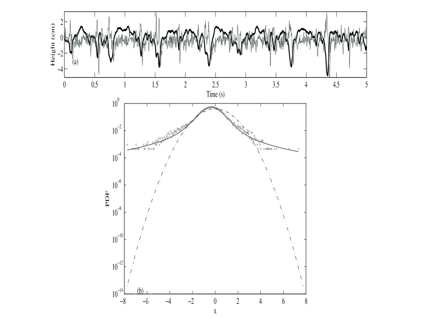
The first line of Tab.1 corresponds to the case I of capillary wind wave slopes at moderate wind speed and at a very short fetch. In this case, we find a stability index of 1.72 that is indicative of a strong non-Gaussian character. A very weak value of the skewness parameter is also found traducing a lack of asymmetry on the waveform. The scale parameter is at a relative low value compared to the normalized Gaussian standard deviation($\sim S_{2}(0,1/\sqrt{2},0)$). This may be related to a nonlinear effect involved on the generation of capillary waves by wind. The characteristics of the capillary wave slopes are shown in Fig.2. The Fig.2.a depicts a sample of the capillary wave profile and its slope while the corresponding probability distribution is shown in the part (b) of the figure with a normalized Gaussian law as a reference.

Figure 2: Fetch=2m. U${}_{\mbox{\tiny{10}}}$ = 6m/s. Part(a): Thick line: Normalized sample of surface wave. Thin line: Normalized instantaneous slope sample. Part(b): ’o’: PDF of slope experiment data. Solid line: $\alpha$ stabe PDF. Dashed-dotted line: Normalized Gaussian PDF

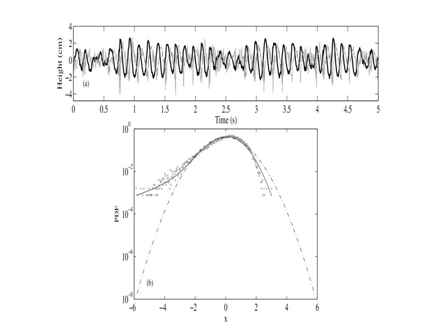
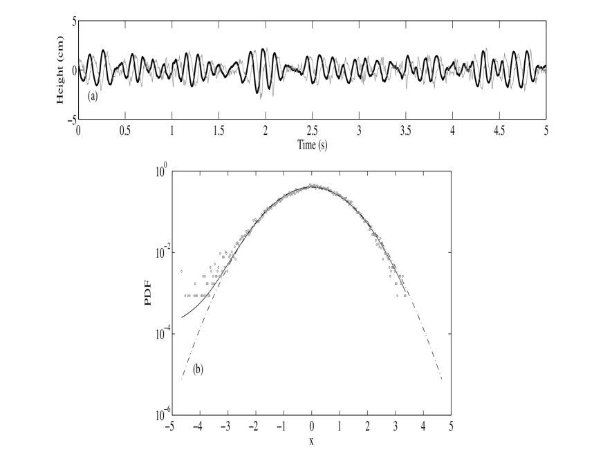
At larger fetch value corresponding to case II, the stability index grows. The scale parameter also increases. A striking feature is that the skewness parameter reaches to its negative limit value. This is in good agreement with time evolution of the slope presented in Fig3.a. Observing also that the corresponding surface waves are dominated by a Stokes component, we suggest the possible role of the Stokes effect in the asymmetric behavior of the slope and in the limit value obtained for the skewness parameter in the present case. However, in the general case, relation between asymmetry in the surface and in the slope variation is not easy to establish especially for a random wavefield. The Stokes effect yields a waveform with steeper crests increasing locally slopes and flatter troughs. Results of run at fetch of 6m and wind speed of 6m/s (case II-1) are shown in Fig.3. The asymmetry property is clearly visible on the slope samples (Fig.3.a) and is well represented by the PDF model (Fig.3.b). Modulational instabilities begin to occur in the wavefield owing to the nonlinear wave-wave interaction processes as the Benjamin-Feir instabilities. The sample of the wave signal presents wave trains formation that are reminiscent of these instabilities effects (see Fig.3.a). Such nonlinear effects are known in this case to dominate the effects of randomness. This would explain the reduction of slope magnitude and also the increase of the stability index to the near-Gaussian situation. By increasing the fetch value but taking a low wind speed (case II-2), the rate of input wind energy will be weaker than the rate of the self-nonlinearity of the wavefield. Thus, one can better put forward the wave modulation effect on the slope distribution and on its PDF. The corresponding PDF is shown in Fig.4.b with a very similar form to the normalized Gaussian except for the negative tail that is indicative of the presence of Stokes effect.

Figure 3: Fetch=6m. U${}_{\mbox{\tiny{10}}}$ = 6m/s. Part(a): Thick line: Normalized sample of surface wave. Thin line: Normalized instantaneous slope sample. Part(b): ’o’: PDF of slope experiment data. Solid line: $\alpha$ stabe PDF. Dashed-dotted line: Normalized Gaussian PDF

Figure 4: Fetch=13m. U${}_{\mbox{\tiny{10}}}$ = 3m/s. Part(a): Thick line: Normalized sample of surface wave. Thin line: Normalized instantaneous slope sample. Part(b): ’o’: PDF of slope experiment data. Solid line: $\alpha$ stabe PDF. Dashed-dotted line: Normalized Gaussian PDF

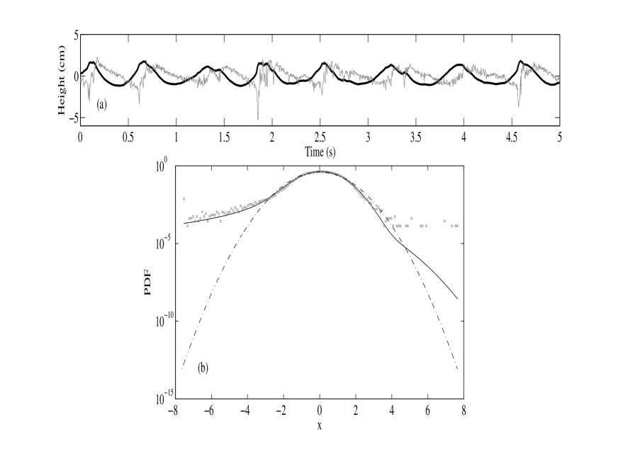
Finally, at high wind speed and large fetch corresponding to the case III, one can surprisingly find that values of the index stability but also the skewness and the scale parameter reduce reaching again a clearly non-Gaussian situation. In agreement with these values, from the Fig.5.a, it may be found that the magnitude of the wave slopes grows locally at the crests and the wave signal behaves strongly asymmetrical. From the physical background, it was shown by Trulsen and DystheTrulsen that such situation may be explained from a theoretical model based on a modified nonlinear Schrödinger equation. It allows one to predict the stabilization of the Stokes effects by the strong wind leading to the suppression of the modulational instabilities. The PDF of the case III are given in Fig.5.b in which it may be found that the stable PDF model reproduce well the distribution of the negative slope values and also the skewness of the slopes. However, at large positive values, the model fails to represent the data distribution. No clear interpretation was found for this difference but we believe that additional physical processes such as breaking wave would be involved.

Figure 5: Fetch=26m. U${}_{\mbox{\tiny{10}}}$ = 13m/s. Part(a): Thick line: Normalized sample of surface wave. Thin line: Normalized instantaneous slope sample. Part(b): ’o’: PDF of slope experiment data. Solid line: $\alpha$ stabe PDF. Dashed-dotted line: Normalized Gaussian PDF

IV Comparison with other models of slope distribution

In this section, we compare the properties of the stable law with the Gram Charlier and the Liu models. The Gram-Charlier model based on an expansion technique called Edgworth series was widely used in the past and permitted to develop a large part of the understanding of the non-Gaussian behavior of the sea surface. However, the limit of this model was earlier found by several authors. Many efforts were conducted to develop alternative ways from the statistical expansion technique. The Liu model was built in this context to improve the statistical representation of the sea surface slopes.

The Gram-Charlier series

The traditional method of interpreting the wind wave slopes has been to fit them to a Gram-Charlier series, which can be derived by assuming that surface waves are weakly nonlinear (Longuet-HigginsLonguet ). Basically, in this procedure the PDF of the wave slopes s(t) writes as:

$$\phi_{\mbox{\tiny{GC}}}(s)=\mbox{G}(s)\left[1+\frac{\mbox{C}_{3}}{6}\mbox{ H}_{3}(s)+\frac{\mbox{C}_{4}}{24}\mbox{ H}_{4}(s)\right]$$ (10)

where

$$\mbox{G}(s)=\frac{1}{\sigma\sqrt{2\pi}}\mbox{ exp }\left[-\left(\displaystyle\frac{s-<s>}{\sqrt{2}\sigma}\right)^{2}\right]$$

and $\sigma$ is the rms of the slope, when $\mbox{H}_{n}$ is the $\mbox{n}^{\mbox{th}}$ Hermite polynomial. The coefficients $\mbox{C}_{n}$ can be calculated from the statistical moments of $\phi_{\mbox{\tiny{GC}}}$(s) and G(s) as:

$$C_{n}=\frac{1}{\sigma^{n}}\displaystyle\int s^{n}\left[\phi_{\mbox{\tiny{GC}}}(s)-\mbox{G}(s)\right]ds$$

Clearly, the coefficients $\mbox{C}_{3}$ and $\mbox{C}_{4}$ in expression (10) are intended to include the skewness and the kurtosis that are the consequences of nonlinearities in the underlying physical processes. Of interest is that the PDF model becomes non-Gaussian. Note also that expression (10) is not always guaranteed to be positive, and is therefore not a valid probability distribution. The Gram-Charlier series diverges in many cases of interest. It converges only if $\phi_{\mbox{\tiny{GC}}}$(s) falls off faster than $\mbox{exp}(-s^{2}/4)$ at infinity (CramérCram ). For water waves applications, the skewness and kurtosis coefficients ($C_{3}$ and $C_{4}$) are found to be related to physical parameters in particular to the air flow speed value at 10m altitude (noted as the $\mbox{U}_{10}$). Here we adopt the values of these coefficients used by Cox & MunkCox and PlantPlant from a range of wind speed varying from 0.72 to 10.2 m/s (Note that Cox uses the wind speed at height of 12.5m instead of the traditional $\mbox{U}_{10}$). We fit the Gram-Charlier model with stable law using the Nelder-MeadNelder simplex method. The results of the fit are given in Tab.2. The method is based on the minimization of the euclidian norm of the error $\epsilon=||\mbox{ f}_{\alpha,\beta,\gamma,\mu}-\phi_{\mbox{\tiny{GC}}}||$ for 1000 points varying from -5 to +5. From each case, values of the best stable parameters and the error $\epsilon$ are shown.

U${}_{\mbox{\tiny{12.5}}}$ (m/s)	$\sigma$	$\mbox{C}_{3}^{{}^{CM}}$	$\mbox{C}_{4}^{{}^{CM}}$	$\alpha$	$\beta$	$\gamma$	$\mu$	$\epsilon$
0.72	0.0005	0.101	0.127	1.951	-0.330	0.695	-0.05	$1e^{-1}$
3.93	0.0098	0.003	0.129	1.957	0.022	0.695	0	$1.9e^{-2}$
4.92	0.0174	-0.080	-0.019	1.980	0.900	0.708	0.040	$8.6e^{-2}$
6.30	0.0170	-0.143	0.101	1.974	0.880	0.697	0.070	$1.5e^{-1}$
8.00	0.0191	-0.156	0.173	1.930	0.260	0.690	0.07	$1.5e^{-1}$
10.2	0.0357	-0.283	0.128	1.910	0.400	0.690	0.13	$2.7e^{-1}$

Table 2: Estimation of stable parameters ($\alpha,\beta,\gamma,\mu$) from the Gram-Charlier series used by Cox and Munk (1954) model

As a general remark for all cases, the values of the stability index $\alpha$ are close to $2$ that traduces the near-Gaussian assumption adopted in the Gram-Charlier model. The error $\epsilon$ increases with the wind speed values. Rather than a simple difference from the calculation, these error values reveal a more profound departure on the nature of both models. More precisely, at low wind speed, when the occurrence of large values of slope would be rare, a better agreement is found in particular around the peak of the PDF.

Figure 6: Results of the fit for U${}_{\mbox{\tiny{12.5}}}$ =8m/s. The solid line is the Gram-Charlier PDF. Dashed line represents the stable law of the fit. A fixed value of the probability is drawn with dotted line that allows one to visualize the asymmetry of both laws.

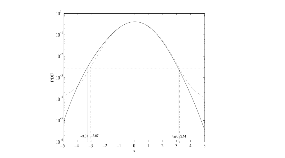
At high wind speed, the results of the Gram-Charlier series differ clearly from those of the stable law both at the tails of the probability and at its middle part. The Gram-Charlier model underestimates the extreme events giving a less heavy tails on the probability law (see Fig.6). At the middle part of probability law, it overestimates the effect of the skewness. Note that no clear tendency is found between the stable parameter $\beta$ and the skewness $\mbox{C}_{3}^{{}^{\mbox{\tiny{CM}}}}$. Finally, the location parameter $\mu$ is globally around zero and the scale parameter $\gamma$ is found at a quasi constant value around $\frac{1}{\sqrt{2}}$. They are directly related to the normalized Gaussian law of the function G(s) included in the expression (10).

The Liu model of slope PDF

A more advanced model is developed by Liu et alLiu to fit the joint probability of the surface wave slopes. Liu model is also based on the weakly nonlinear assumption of the surface Longuet . The basic form of Liu slope PDF writes as:

$$f_{L}^{n}(x,y)=\frac{n}{2\pi(n-1)}\left[1+\frac{x^{2}}{(n-1)}+\frac{y^{2}}{(n-1)}\right]^{-(n+2)/2}$$ (11)

where x,y are normalized slope components and n an integer parameter describing the peakedness of the surface slopes. Note that (11) refers to the case of isotropic sea surface and is not always suitable for anisotropic real surface. An empirical formulation inspired by Cox Longuet is used by Liu to handle the skewness effect. According to Liu , the expression (11) is an improvement of the Gram-Charlier distribution in particular for the range of large slopes. For convenience, here we consider the expression for y=0, i.e. we focus only on upwind direction. As a first remark, the positivity of the expression (11) is obviously guaranteed however it may be found that the expression of $f_{L}^{n}(x,0)$ does not represent a valid probability density function for any value of n. Indeed, the integral of this expression is not equal to unity. We addres this point by adopting a normalized form of the Liu PDF as:

$$\phi_{L}^{m}(x)=\frac{1}{\sqrt{\pi}}\left[1+\frac{x^{2}}{(m-1)}\right]^{(-\frac{m}{2}+1)}\displaystyle\frac{\Gamma(\frac{m}{2}-1)\sqrt{\frac{1}{m-1}}}{\Gamma(\frac{m}{2}-\frac{3}{2})}$$ (12)

The expression (12) is defined for $m\geq 4$. For m=4, one can easily find that

$$\phi_{L}^{4}(x)=\frac{1}{\pi}\left(\frac{\sqrt{3}}{3+x^{2}}\right)$$ (13)

Expression (13) belongs to the Cauchy stable law with $\mbox{X}\sim S_{1}(0,\sqrt{3},0)$. On the other hand, taking the logarithm of (12), the limit for large value of m writes as:

$$\mbox{log }\phi_{L}^{m}(x)\displaystyle\simeq_{m\rightarrow\infty}-\frac{m-2}{2}\mbox{ log}\left(1+\frac{x^{2}}{m-1}\right)$$ (14)

which reaches by simple series expansion to the normal distribution of $\mbox{X}\sim{\cal N}(0,1)$ or also the stable law with $\mbox{X}\sim S_{2}(0,\frac{1}{\sqrt{2}},0)$. The limit cases of the Liu formulation belong to the symmetrical stable distribution.

For intermediate values, the Liu PDF differs slightly from the stable distribution. In order to illustrate this relation, we compute a numerical adjustment of the stable parameters $\alpha$ and $\gamma$ to the expression (12) for m=4.5. The adjustment is based on the minimization of the euclidian norm $||\mbox{ f}_{\alpha,0,\gamma,0}(x)-\phi_{L}^{m}(x)||\leq\epsilon$ for 3000 points from x=-15 to 15. The results are shown in Fig.7. It may be found that the major difference between the two laws are clearly localized at the medium range values of the probability structure.

Figure 7: Semi-log representation of Liu PDF for m=4.5 and the stable law fit with $\alpha=1.221$ and $\gamma=1.3384$. The error $\epsilon=0.066277$. Solid line: Liu PDF model. Dashed line: Stable law.

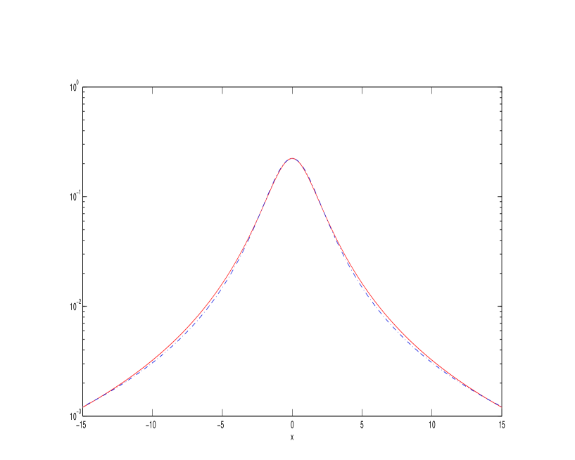
By varying the peakedness parameter m, this difference is retained systematically. Analytically, one can also decompose the modified Liu model to study its property. As an example, taking m=6, the Liu PDF writes as:

$$\phi_{L}^{6}(x)=\frac{1}{\pi}\frac{\sqrt{5}}{5+x^{2}}+\frac{1}{\pi}\frac{\sqrt{5}(5-x^{2})}{(5+x^{2})^{2}}$$ (15)

where the first term is a Cauchy law $S_{1}(0,\sqrt{5},0)$. As shown from the Fig.8, the second term possesses a significant positive values at the middle and the medium parts of the probability law. The magnitude of these positive values are responsible of the height of Liu PDF and the departure from the stable law at the medium range values. The negative values of the second term of (15) explain the similarity of the asymptotic behavior of both laws observed in Fig.7.

Figure 8: The corresponding figure of expression (15). The Cauchy law (first term) is on dashed line while solid line represents the second term with negative part. The zero value is drawn with dotted line

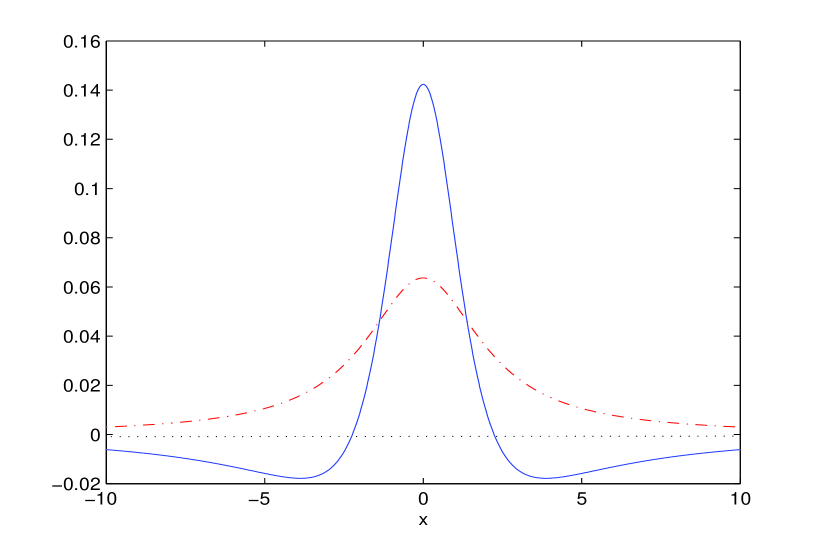
For higher values of m, the same expansion holds with a Cauchy law $S_{1}(0,\sqrt{m-1},0)$ as a first term but the second term becomes a sum of rational functions whose integral vanishes to ensure the normalization of the PDF.

According to the probability theory, the modified Liu PDF belongs to the family of the Generalized Student or T-distribution whose expression writes as:

$$\phi_{S}^{m}(x)=\displaystyle\frac{\Gamma(m+\frac{1}{2})}{\Gamma(\frac{m}{2})\quad\Gamma(\frac{1}{2})}\left(\frac{a}{(x^{2}+a^{2})^{m+\frac{1}{2}}}\right)$$ (16)

where m is now called freedom degrees and a is a scale parameter. The characteristic function of the T-distribution is given by:

$$\psi_{S}^{m}(t)=\quad 2\displaystyle\frac{|\mbox{at}|^{\frac{m}{2}}\quad\displaystyle K_{\frac{m}{2}}(|\mbox{at}|)}{2^{\frac{m}{2}}\Gamma(\frac{m}{2})}$$ (17)

where $K_{i}$ is the modified Bessel function. From (2) and (17), one can evaluate the difference between the stable and the T-distribution laws. As said in previous section, the stable laws decay as $|x|^{-\alpha-1}$ with $\alpha<2$. Here, it may be shown that the T-distribution laws have the same asymptotic behavior as $|x|^{-m-1}$ for all m$>$0. Note that as a consequence, the T-distribution laws are more accurate than the stable laws to approximate the near-Gaussian situation. Another significant difference concerns the variance of the laws: for all m$>$2, the T-distribution laws have finite variance given by $\sigma^{2}=\frac{a^{2}}{m-2}$ while the stable laws do not possess finite variance except only for $\alpha=2$. From the practical viewpoint, this lack of variance may be of crucial importance when one has to compute statistical values as the mean square slope that is necessary to evaluate the radar backscatter cross section.

Finally, from the expression (16), it appears that the T-distribution does not include a skewness property while the stable laws are naturally able to express the skewness effect. Recalling the importance of the skewness effect on the dynamic of the surface waves, this point may have significant consequences on the accuracy of the slope distribution model.

V Conclusion

The main purpose of this study was to highlight the possible use of $\alpha$-stable laws for water surface slopes representation. As said in the introduction of this paper, the fundamental argument on the use of $\alpha$-stable laws stems first from experimental observations of the main property of the wind driven water surface waves: a possible fractal representation, related to a spectral power law, nonlinear characters of the wind wavefield resulting in an asymmetry and a modulational instability of the surface, and a randomness of the slope, such as these abrupt changes shown here in section 3.

Considering these strongly disordered behaviors that may be found on slope variations, $\alpha$-stable laws seem à priori to be potential candidates for this objective. Starting from this idea, the study propose to apply the stable laws to represent the probability distribution of the slopes of wind driven water surface from laboratory experiments. It is found that the stable laws are well adapted to model the random characteristic of the slopes data in different cases of experiment configurations. From the proposed cases, the four stable parameters behave in good agreement with the effects of different physical processes observed and expected in the experiments. In particular, the stability index traduces fairly the non-Gaussianity of the slopes in the same sense as the Stokes and/or the modulational instability effects. Also the skewness parameter reproduces well the asymmetry tendency of the slopes under various situations. However, at extreme experiment condition (large fetch and high wind speed), the stable laws fail to reproduce the behavior of the upper part of the slopes.

From more theoretical consideration, comparisons with the Gram-Charlier and the Liu et alLiu models are carried out. It appears that the stable law differs completely from the Gram-Charlier model as well as in its mathematical structure than from the characteristics of its results. Indeed, one can recall that the Gram-Charlier model at its usual truncation order (third or fourth order) is part of the near-Gaussian approximation models, while the stable law is totally non-Gaussian except only when the stability index reaches its maximum value.

The comparison with the Liu model shows more similarities. Recalling that Liu model belongs to the T-distribution family, it is well established that both models are part of the so-called ”heavy tail probability laws”. They are both infinitely divisible probability laws but the T-distribution is not stable. This means that the sum of independent identically T-distributed variables does not follow the same law unlike the stable law that it is always the case.

From mathematical viewpoint such stability property lies onto fundamental characteristic based on the generalization of the central limit theorem (see Samorodnitsky and TaqquSamor ) and traduces the fact that the $\alpha$-stable laws constitute limit laws (or attractor laws) for all additive random processes. As a special case, we recall that for $\alpha=2$, from the central limit theorem, the Gaussian law is a limit law for all additive finite variance random processes. This is the profound justification of the popularity of the Gaussian model in many physical domains. In the realm of water surface waves, the random wavefield is usually considered as the sum of infinite number of random components. Owing to the weakness of the interactions between components, the corresponding motion of each component may be regarded as independent (see for example Phillips Phil ). Consequently, under the generalisation of the central limit theorem, the choice of stable law is then theoretically justified with a clear mathematical basis.

With regard to the practical viewpoint, the differences between the two laws are more important and have to be stressed here with respect to the study objective. These differences lie on four points concerning the closed form of the PDF, the finite variance value, the skewness representation and the interpretation of the physical processes through the PDF parameters.

As said in previous section, the T-distribution has a closed form of the PDF for all values of its parameters . There are only three cases of stable distributions for which a closed form expression of the PDF is known. This lack of closed form is apparently an inconvenient property of the stable law. However, as shown in this study, there exists robust techniques to implement the integral form of the stable PDF (see Zolotarev zol , WeronWeron , NolanNolan ). Other expansion techniques based on the Bergström series are also available to evaluate the stable PDF.

For physical applications, an appeal to statistical quantities associated with the PDF model would be useful. For example, for the sea surface remote sensing problem, it is known that the mean and the variance of the slopes are of importance. This is historically related to the assumption of near-Gaussian state in the development. Recalling that T-distribution has finite variance for all freedom degrees greater than 2. T-distribution appears as a well adapted choice for this purpose. However, the T-distribution and the stable distribution constitute fully non-Gaussian alternative and then fail to belong to the category of quasi-Gaussian solutions. In our opinion, an extension of the remote sensing or the hydrodynamical relationships in the sense as developed by Guéringuerin is required for a fully non-Gaussian solution.

As far as non-Gaussian random water surface is concerned, the skewness is undoubtedly one of its most important properties. The stable distribution has asymmetric form that allows one to include naturally the skewness. This is not the case of the T-distribution for which no extension to asymmetric case is previewed. Empirical asymmetric formulation has to be found (see Liu et alLiu ).

Before ending the paper, we focus on the interpretation of the physical processes through the probability distribution model. As we have shown in this study, the four stable parameters are able to traduce correctly the effects of physical processes as the asymmetry and the kurtosis of the slopes or also its level of non-Gaussianity. Use of $\alpha$-stable distribution instead of the traditional Gaussian or quasi-Gaussian distributions, combined to hydrodynamical laws will be of great help on understanding the physical behavior of the water wave slopes. In this sense, extension of the present work to the space representation of water wave slopes by the use of multivariate $\alpha$-stable distribution has to be carried out and constitutes our prospective task. An other way to be explored is also the use of truncated stable law that allows one to obtain finite values of statistical moments.

Acknowledgements The authors are particularly grateful to Yuri Stepanyants and to Fred Ramamonjiarisoa for their helpful discussions on the first draft of this manuscript. The authors thank also E. Michel for his help to improve the text.

References

- (1) Borak S., Härdel W. and Weron R. 2005 ”Stable Distribution”, SFB 649 Discussion Paper 2005-008
- (2) Chapron, B., V. Kerbaol, D. Vandemark, and Elfouhaily T. 2000, ”Importance of peakedness in sea surface slope measurements and applications”, J. Geophys. Res., vol. 105(C7), 17195 17202.
- (3) Coantic M. and Favre A. 1974 ”Activities and preliminary results of air-sea interaction research at IMST”, Advances in Geophysics, 10, 391.
- (4) Cox C. and Munk W. 1954 ”Statistics of sea surface derived from sun glitter”, Journal of Marine Research, 13, 199-227.
- (5) Cox C. and Munk W. 1956 ”Slopes of sea surface deduced from photographs of sun glitter”, Bull. of Scripps Institution of Oceanography, vol.6, 401-488.
- (6) Cramér H. 1957. ”Mathematical Methods of Statistics”. Princeton University Press, Princeton.
- (7) Guérin C.A. 2002. ”Scattering on rough surface with -stable non-Gaussian height distributions”. Waves in Random Media, vol. 12, 293-306.
- (8) Huang N. 1991,”The local properties of ocean surface waves by the phase-time method”, in Nonlinear Water Waves Workshop, University of Bristol.
- (9) Jähne B. and Riemer K.S. 1990 ”Two-dimensional wave number spectra of small scale water surface waves”, Journal of Geophysical Research, 95, 11531-11546.
- (10) Joelson M.,Dudok de Wit T.,Dussouliez P. and Ramamonjiarisoa A.,2000, ”Searching for chaotic and deterministic features in laboratory water surface waves”, Nonlinear Processes in Geophysics, vol.7, 37-48.
- (11) Kogon, S.M.and Williams D.B. 1998 ”Characteristic function based estimation of stable parameters”, in A Practical Guide to Heavy Tails, eds. R. Adler, R.Feldman, and M. Taqqu (Birkhauser, Boston).
- (12) Koutrouvelis I.A. 1980 ”Regression-Type Estimation of the Parameters of Stable Laws”, Journal of The American Statistical Association 75, 918-928.
- (13) Leykin I.A.,Donelan M.A.,Mellen R.H. and McLaughlin D.J.,1995 ”Asymmetry of wind waves studied in a laboratory tank”, Nonlinear Processes in Geophysics, vol.2, 280-289.
- (14) Lévy P.,1925, ”Calcul des probabilités”,Paris, Ed. Gauthier Villars.
- (15) Liu Y. Yan X.H. Liu W.T. and Hwang P. A. 1997 ”Probability Density Function of Ocean Surface Slopes and Its Effects on Radar Backscatter”, Journal of Physical Oceanography, 27, 782-797.
- (16) Longuet-Higgins M.S. 1963 ”The effect of nonlinearities on statistical distributions in theory of sea waves”, Journal of Fluid Mechanics, 16, 138-159.
- (17) Mellen R.H. and Leykin I.A. 1994,”Nonlinear dynamics of wind waves: multifractal phase/time effects”, Nonlinear Processes in Geophysics, vol.1, 51-56.
- (18) Nelder J. A. and Mead R., 1965, ”A simplex Method for function minimization”, Computer Journal 7, 308-313.
- (19) Nolan J.P., 1997 Numerical ”Calculation of Stable Densities and Distribution Functions” Communications in Statistics - Stochastic Models, Vol.13, pp. 759-774.
- (20) Onorato M., Osborne R., Serio M., Brandini C., Stansberg C.T., 2004 ”Observation of strongly non-Gaussian statistics for random sea surface gravity waves in wave flume experiments”, Phys. Rev. E, Vol.70, 067302.
- (21) Plant J.W. 2003 ”A new interpretation of sea-surface slope probability density functions”, Journal of Geophysical Research, 108, 3295-3299.
- (22) Phillips O.M. 1977 ”The dynamics of the Upper Ocean”, 2nd edn, Cambridge University Press.
- (23) Samorodnitsky, G. and Taqqu, M.S. 1994. ”Stable Non-Gaussian Random Processes”, Chapman and Hall.
- (24) Solow A.R. 2005,”Power law without complexity”, Ecology Letters, vol.8, 361-363.
- (25) Soriano G., Joelson M. and Saillard M. 2006, ”Doppler spectrum from two-dimensional ocean surface at microwave frequency”, IEEE Trans. Geoscience and Remote Sensing, Vol.44, 2430-2437.
- (26) Trulsen, K. and Dysthe, K.B. 1992. ”Action of windstress and breaking on the evolution of a wavetrain”, in ”Breaking Waves”, eds Banner and Grimshaw, Springer, 243 249.
- (27) Valenzuela, G. R., 1978. ”Theories for the interaction of electromagnetic and ocean wave-A review”. Bound.-Layer Meteor., Vol.13, 61-85.
- (28) Warnick K.F.,Millet F.W. and Arnold D.V. 2005. ”Physical and Geometrical Optics for 2-D Rough surfaces with power-law height spectra”, IEEE Transactions on Antennas and Propagation, vol. 53, num.3,922-932.
- (29) R.Weron 1995 ”Performance of the estimators of stable law parameters”,Research Report HSC/95/1, http://www.im.pwr.wroc.pl/ hugo/Publications.html
- (30) R.Weron, 2004 ”Computationally intensive Value at Risk calculations”, in ”Handbook of Computational Statistics: Concepts and Methods”, eds. J.E. Gentle, W. Haerdle, Y. Mori, Springer, Berlin, 911-950.
- (31) Zolotarev, M.V. 1986. ”One dimensional Stable Distributions”, Amer. Math. Soc., Vol 65 (Transl. of the original 1983 Russian).