MPP-2008-98
MZ-TH/08-28
TTP-08-44
SFB-CPP-08-79

Hadronic top-quark pair production
in association with a hard jet at next-to-leading order QCD:
Phenomenological studies for the Tevatron and the LHC

S. Dittmaier¹, P. Uwer² and S. Weinzierl³

¹ Max-Planck-Institut für Physik (Werner-Heisenberg-Institut),
D-80805 München, Germany

² Institut für Theoretische Teilchenphysik,
Universität Karlsruhe, D-76128 Karlsruhe, Germany

³ Institut für Physik,
Universität Mainz, D-55099 Mainz, Germany

We report on the calculation of the next-to-leading order QCD corrections to the production of top–antitop-quark pairs in association with a hard jet at the Tevatron and at the LHC. Results for integrated and differential cross sections are presented. We find a significant reduction of the scale dependence. In most cases the corrections are below 20% indicating that the perturbative expansion is well under control. Moreover, the forward–backward charge asymmetry of the top-quark, which is analyzed at the Tevatron, is studied at next-to-leading order. We find large corrections suggesting that the definition of the observable has to be refined.

October 2008

1 Introduction

The top-quark is by far the heaviest elementary fermion in the Standard Model (SM). With a mass of $(172.6\pm 1.4)$ GeV [1] its mass is about 36 times larger than the mass of the next heaviest fermion, the bottom quark. The large mass has lead to various speculations whether the top-quark behaves as a normal quark or whether it plays a special role in particle physics. The electroweak SU(2)$\times$U(1) gauge structure of the SM, which is successful in describing a large variety of measurements, would require the quark masses to be zero if the symmetry was un-broken. With the largest mass amongst the quarks it is thus natural to assume that the top-quark is most sensitive to the mechanism of electroweak symmetry breaking. In particular, the fact that the top-quark mass is close to the scale of electroweak symmetry breaking—or equivalently, that the Yukawa coupling to the Higgs is very close to one—has motivated different scenarios in which the top-quark drives the electroweak symmetry breaking. More details can be found in recent review articles [2, 3].

Ignoring the SM as the theory of particle physics one might still wonder whether the top-quark, which is almost as heavy as a gold atom, behaves as a point-like particle. A deviation from the point-like nature would appear as anomalous moments yielding differential distributions different from the point-like case. Anomalous couplings to the gluon are most naturally probed via the production of an additional jet. An indirect measurement through the measurement of the total cross section is in general more difficult. This is in particular true when the interference term with the corresponding Born amplitude gives no contribution to the total cross section due to discrete symmetries.

In the context of the SM we have the remarkable fact that the electroweak top-quark interactions are completely determined through the aforementioned SU(2)$\times$U(1) gauge structure of the SM. The only free parameter appearing in top-quark physics is thus the top-quark mass or equivalently the Yukawa coupling to the Higgs boson. Once this parameter is measured all remaining properties are predicted.

An important task for the ongoing Tevatron collider and the recently started LHC is the precise measurement of the top-quark properties. The ultimate goal is to measure the spin and the quantum numbers of the top-quark as precisely as possible. Any deviation from the SM would signal new physics. There is a variety of measurements which are currently done at the Tevatron and will be continued at the LHC. The total cross section, which is currently measured at the Tevatron with an accuracy of about 10% [4], is expected to be measured at the LHC with an accuracy of 5%. This measurement allows to make precise tests of the production mechanism. Other important measurements comprise the cross section for single top-quark production [5, 6, 7, 8, 9, 10, 11], the W-polarisation in top-quark decay or the spin correlations of top-quark pairs [12, 13, 14, 15, 16, 17, 18, 19, 20]. Of great interest is also the electric charge of the top-quark and its couplings to the Z-boson and the Higgs boson. They can be constrained via the measurements of the cross sections for ${\mathrm{t}}\bar{\mathrm{t}}\gamma$, ${\mathrm{t}}\bar{\mathrm{t}}Z$ [21], and ${\mathrm{t}}\bar{\mathrm{t}}H$ [22, 23, 24, 25] production.

The production of a top-quark pair together with an additional jet is a further important reaction. This becomes already clear from the simple observation that a substantial number of events in the inclusive top-quark sample is accompanied by an additional jet. Depending on the energy of the additional jet the fraction of events with an additional jet can easily be of the order of 10–30% or even more. For example at the LHC we find a cross section of 376 pb for the production of a top–antitop-quark pair with an additional jet with a transverse momentum above 50 GeV. This is almost half of the total top-quark pair cross section which is 806 pb [26] if evaluated in next-to-leading order (NLO). For a more precise understanding of the topology of top-quark events it is thus important to have also an improved understanding of top-quark pair production together with a jet. As mentioned already above, this reaction provides a sensitive tool to search for anomalous top-quark–gluon couplings. The emission of an additional gluon also leads to a rather interesting property of the cross section: The differential cross section contains contributions from the interference of C-odd and C-even parts of the amplitude[27, 28, 29, 30], where C denotes the charge conjugation (for a similar effect in QED see for example Refs. [31, 32]). While for the total cross section these contributions cancel when integrating over the (symmetric) phase space they can lead to a forward–backward charge asymmetry of the top-quark which is measured at the Tevatron [33, 34]. It should be stressed that no parity-violating interactions are involved. Note that the naively defined forward–backward charge asymmetry is zero at the LHC due to the symmetric initial state. A definition that leads to a non-trivial prediction here requires to select a preferred axis for each event[35], but it is not yet clear whether an asymmetry survives that is significant over all uncertainties. In inclusive top-quark pair production at the Tevatron the charge asymmetry appears first at one loop, because it results from interferences of C-odd with C-even parts of double-gluon exchange between initial and final states. The asymmetry for the inclusive sample has been studied in detail in Refs. [27, 28, 29, 30]. The available predictions for ${\mathrm{t}}\bar{\mathrm{t}}$ production—although of one-loop order—describes this asymmetry only at leading-order (LO) accuracy in QCD. Recently the analysis has been extended to take large threshold logarithms at the next-to-leading-log (NLL) level into account [36]. It was found that at least this class of higher-order contributions do not change the theoretical prediction dramatically. The main reason is that this type of corrections affect the asymmetric cross section roughly in the same way as the symmetric one. In the ratio the corrections thus cancel to a large extent and lead to a stable theoretical prediction. In ${\mathrm{t}}\bar{\mathrm{t}}{+}$jet production the asymmetry appears already in the tree amplitude. Thus, the NLO calculation described in this article provides a true NLO prediction for the asymmetry. The calculation presented in this work is an important tool in the experimental analysis of this observable at the Tevatron where the asymmetry is measured [33, 34]. In a previous letter [37] we reported that the asymmetry receives large corrections. In this paper we study the situation in more detail for various values of the lower cut on the transverse momentum of the hard tagging jet.

As aforementioned it is expected that the total cross section for top-quark pair production will be measured at the LHC with an accuracy of the order of 5%. Recently it has been shown in Refs. [26, 38, 39] that the accuracy of the currently available NLO predictions is only at the level of 12% (at NLO, but further reduced by the inclusion of the threshold logarithms) and largely dominated by the scale uncertainty. In Ref. [26] an estimate to the next-to-next-to-leading order (NNLO) cross section has been given. The approximation is based on the assumption that the NNLO corrections will be dominated by the threshold region as it is the case for the NLO corrections. In the threshold region the logarithmic behaviour together with the two-loop Coulomb singularity is derived from general arguments. In addition the complete scale dependence at two loops is included in the approximation. Using this approximation to the full NNLO result it is shown in Ref. [26] that the theoretical uncertainty may decrease to a few per cent. The remaining scale uncertainty is of the same order as the uncertainty induced by the parton distribution functions. Recently some progress towards a complete NNLO calculation has been made [40, 41, 42, 43, 44, 45, 46, 47, 48]. The one-loop corrections to ${\mathrm{t}}\bar{\mathrm{t}}+{\mbox{1-jet}}$ constitute an important ingredient to the NNLO calculation of ${\mathrm{t}}\bar{\mathrm{t}}$ production at hadron colliders. In this context we mention that—besides our NLO calculation presented here and in Ref. [37]—part of the one-loop amplitudes to ${\mathrm{g}}{\mathrm{g}}\to{\mathrm{t}}\bar{\mathrm{t}}{\mathrm{g}}$ have also been evaluated in Ref. [49].

Apart from its significance as signal process it turns out that ${\mathrm{t}}\bar{\mathrm{t}}+{\mbox{1-jet}}$ production is also an important background to various new physics searches. A prominent example is Higgs production via vector-boson fusion. This reaction represents an important discovery channel for a SM Higgs boson with a mass of up to several $100\,\mathrm{GeV}$ [50, 51]. The major background to this reaction is due to ${\mathrm{t}}\bar{\mathrm{t}}+{\mbox{1-jet}}$ [52], again underlining the need for precise theoretical predictions for this process.

It is well known that predictions at LO in the coupling constant of QCD are plagued by large uncertainties. In many cases the LO predictions in QCD give only a rough estimate. Only by including NLO corrections a quantitatively reliable prediction can be obtained. Given that the conceptual problems in such calculations are solved since quite some time, one might think that doing the required calculations should be a straightforward task. Unfortunately it turns out that this is not the case. The calculation of radiative corrections for $2\to 3$ and $2\to 4$ reactions is still non-trivial—not speaking about reactions with an even higher multiplicity. The complexity of the corresponding matrix elements renders computer codes quite lengthy and CPU time consuming. The (more or less) automatically generated code may in addition lead to numerical instabilities. In particular, the reduction of one-loop tensor integrals to scalar one-loop integrals is in general difficult to do in a numerically stable way. In that context the calculation of the one-loop corrections to top-quark pair production with an additional jet is also interesting as a benchmark process for the development of new methods.

In this paper we extend our previous work [37] on the NLO QCD corrections to ${\mathrm{t}}\bar{\mathrm{t}}{+}$jet production at hadron colliders, where we discussed the scale dependence of the integrated cross sections at the Tevatron and the LHC and of the top-quark charge asymmetry at the Tevatron. We supplement this discussion upon including more numerical results showing the dependence on the lower cut set on the transverse momentum of the hard tagging jet and present first results on differential distributions. Moreover, we provide numerical results on the virtual one-loop and real-emission corrections for single phase-space points, in order to facilitate future comparisons to our calculation.

This article is organized as follows: In Section 2 we briefly describe the calculation of the NLO corrections. Numerical results are presented in Section 3. In the appendices we provide numerical results on the virtual and real corrections for individual phase-space points; moreover, we collect the tables with the results for the differential cross sections there.

2 Outline of the calculation

2.1 Born approximation

In Born approximation the partonic reactions are

$${\mathrm{g}}{\mathrm{g}}\to{\mathrm{t}}\bar{\mathrm{t}}{\mathrm{g}},\quad q\bar{q}\to{\mathrm{t}}\bar{\mathrm{t}}{\mathrm{g}},\quad q{\mathrm{g}}\to{\mathrm{t}}\bar{\mathrm{t}}q,\quad{\mathrm{g}}\bar{q}\to{\mathrm{t}}\bar{\mathrm{t}}\bar{q}.$$ (2.1)

The last three reactions are related by crossing. Therefore, the required generic matrix elements are

$$0\to{\mathrm{t}}\bar{\mathrm{t}}{\mathrm{g}}{\mathrm{g}}{\mathrm{g}},\quad 0\to{\mathrm{t}}\bar{\mathrm{t}}q\bar{q}{\mathrm{g}}.$$ (2.2)

In the following we generically denote the external momenta and helicities with $\{p_{i}\}$ and $\{\lambda_{i}\}$ and identify the light partons with $i=1,2,3$. The letter of a specific parton if used as an argument denotes the combination of spin, momentum, and (if relevant) colour of this parton, i.e. ${\mathrm{t}}=(p_{{\mathrm{t}}},\lambda_{{\mathrm{t}}},i_{{\mathrm{t}}})$ or ${\mathrm{g}}_{i}=(p_{i},\lambda_{i},a_{i})$. Representative sets of Born diagrams for the ${\mathrm{g}}{\mathrm{g}}$ and $q\bar{q}$ channels are depicted in Figure 2.1.

                    

             

Figure 2.1: Representative sets of LO diagrams for ${\mathrm{g}}{\mathrm{g}}$ fusion and $q\bar{q}$ annihilation in hadronic ${\mathrm{t}}\bar{\mathrm{t}}{+}$jet production.

In total, there are 16 LO diagrams for $0\to{\mathrm{t}}\bar{\mathrm{t}}{\mathrm{g}}{\mathrm{g}}{\mathrm{g}}$ and 5 for $0\to{\mathrm{t}}\bar{\mathrm{t}}q\bar{q}{\mathrm{g}}$. The colour decomposition for a tree amplitude corresponding to the process $0\to{\mathrm{t}}\bar{\mathrm{t}}{\mathrm{g}}{\mathrm{g}}{\mathrm{g}}$ is

$${\cal A}_{5}^{(0)}({\mathrm{t}},{\mathrm{g}}_{1},{\mathrm{g}}_{2},{\mathrm{g}}_{3},\bar{\mathrm{t}}) = g_{\mathrm{s}}^{3}\sum\limits_{\sigma\in S_{3}}\left(T^{a_{\sigma_{1}}}T^{a_{\sigma_{2}}}T^{a_{\sigma_{3}}}\right)_{i_{{\mathrm{t}}}j_{\bar{\mathrm{t}}}}A_{5}^{(0)}({\mathrm{t}},{\mathrm{g}}_{\sigma_{1}},{\mathrm{g}}_{\sigma_{2}},{\mathrm{g}}_{\sigma_{3}},\bar{\mathrm{t}}),$$ (2.3)

where $g_{\mathrm{s}}$ is the strong coupling constant, $S_{3}$ the symmetric group and $\sigma=(\sigma_{1},\sigma_{2},\sigma_{3})\in S_{3}$ a permutation. The generators of the SU(N) gauge group in the fundamental representation are given by $T^{a}$, and $a_{i}$ is the colour index of gluon ${\mathrm{g}}_{i}$. The sum extends over all permutations in $S_{3}$. Physically this corresponds to all possible colour orderings of the gluons. The function $A_{5}^{(0)}({\mathrm{t}},{\mathrm{g}}_{1},{\mathrm{g}}_{2},{\mathrm{g}}_{3},\bar{\mathrm{t}})$ is thus the colour-ordered subamplitude often also called partial amplitude. Due to the colour-ordering, only diagrams with a particular ordering contribute to $A_{5}^{(0)}({\mathrm{t}},{\mathrm{g}}_{1},{\mathrm{g}}_{2},{\mathrm{g}}_{3},\bar{\mathrm{t}})$. The partial amplitudes contain the kinematic information and are individually gauge invariant. The corresponding colour decomposition for the process $0\to{\mathrm{t}}\bar{\mathrm{t}}q\bar{q}{\mathrm{g}}$ reads

$${\cal A}_{5}^{(0)}({\mathrm{t}},\bar{\mathrm{t}},q,\bar{q},g) = g_{\mathrm{s}}^{3}\left[\frac{1}{2}\delta_{i_{{\mathrm{t}}}j_{\bar{q}}}T^{a}_{i_{q}j_{\bar{\mathrm{t}}}}A_{5,1}^{(0)}({{\mathrm{t}},\bar{\mathrm{t}},q,\bar{q},g,})+\frac{1}{2}\delta_{i_{q}j_{\bar{\mathrm{t}}}}T^{a}_{i_{{\mathrm{t}}}j_{\bar{q}}}A_{5,2}^{(0)}({{\mathrm{t}},\bar{\mathrm{t}},q,\bar{q},g,})\right.$$ (2.4)

$$\left.-\frac{1}{2N}\delta_{i_{{\mathrm{t}}}j_{\bar{\mathrm{t}}}}T^{a}_{i_{q}j_{\bar{q}}}A_{5,3}^{(0)}({{\mathrm{t}},\bar{\mathrm{t}},q,\bar{q},g,})-\frac{1}{2N}\delta_{i_{q}j_{\bar{q}}}T^{a}_{i_{{\mathrm{t}}}j_{\bar{\mathrm{t}}}}A_{5,4}^{(0)}({{\mathrm{t}},\bar{\mathrm{t}},q,\bar{q},g,})\right].$$

We note that the amplitudes $A_{5,i}^{(0)}$ ($i=1,2,3,4$) are linearly dependent. The relation

$$0=A_{5,1}^{(0)}+A_{5,2}^{(0)}-A_{5,3}^{(0)}-A_{5,4}^{(0)}$$

can be used to express for example $A_{5,4}^{(0)}$ in terms of $A_{5,i}^{(0)}$ with $i=1,2,3$. This is particularly useful for the evaluation of the squared amplitude. Compact analytic results for the LO amplitudes are given in Ref. [20] where the amplitudes have been used in the calculation of the NLO corrections for top-quark pair production. In addition we also performed several independent calculations, including one with Madgraph [55], and found complete numerical agreement among all those calculations.

2.2 Virtual corrections

The virtual corrections consist of the one-loop corrections to the LO reactions. One can classify the corrections into self-energy, vertex, box-type, and pentagon-type corrections where all the external legs are directly connected to the loop thus forming a pentagon. The latter are the most complicated ones due to their complexity and the involved tensor integrals. Typical examples of the pentagon graphs are shown in Figure 2.2.

             

             

Figure 2.2: Representative sets of pentagon diagrams for ${\mathrm{g}}{\mathrm{g}}$ fusion and $q\bar{q}$ annihilation in hadronic ${\mathrm{t}}\bar{\mathrm{t}}{+}$jet production at NLO QCD.

Specifically, there are 24 pentagons for $0\to{\mathrm{t}}\bar{\mathrm{t}}{\mathrm{g}}{\mathrm{g}}{\mathrm{g}}$ and 8 for $0\to{\mathrm{t}}\bar{\mathrm{t}}q\bar{q}{\mathrm{g}}$. The total number of diagrams is 354 for the $0\to{\mathrm{t}}\bar{\mathrm{t}}{\mathrm{g}}{\mathrm{g}}{\mathrm{g}}$ case and 94 for the $0\to{\mathrm{t}}\bar{\mathrm{t}}q\bar{q}{\mathrm{g}}$ case. The challenging step in this context is the numerically fast and stable reduction of the tensor integrals to scalar one-loop integrals.

Before describing the details we briefly outline the general setup. Owing to the involved kinematics the individual Feynman diagrams lead to large expressions which are cumbersome to evaluate. To be able to handle the large expressions and to ensure a fast numerical evaluation at the end we used a decomposition of the amplitude according to the spin and colour structure. Schematically the decomposition of the one-loop amplitude ${\cal A}^{(1)}_{5}$ reads

$${\cal A}^{(1)}_{5}=\sum_{c,s}{\cal C}_{c}\times{\cal S}_{s}(\{p_{i}\},\{\lambda_{i}\})\times f^{(1)}_{cs}(\{p_{i}\cdot p_{j}\}),$$ (2.5)

where ${\cal C}_{c}$ denote the colour structures, ${\cal S}_{s}$ are the spin structures (elsewhere called “standard matrix elements”), and the functions $f^{(1)}_{cs}$ are scalar functions that depend only on the scalar products of the external momenta $p_{i}$. In detail, for $0\to{\mathrm{t}}\bar{\mathrm{t}}{\mathrm{g}}{\mathrm{g}}{\mathrm{g}}$ there are 10 independent colour structures ${\cal C}_{c}$ of the form

$$\left(T^{a_{\sigma_{1}}}T^{a_{\sigma_{2}}}T^{a_{\sigma_{3}}}\right)_{i_{{\mathrm{t}}}j_{\bar{\mathrm{t}}}},\qquad\left(T^{a_{\sigma_{1}}}\right)_{i_{{\mathrm{t}}}j_{\bar{\mathrm{t}}}}\delta^{a_{\sigma_{2}}a_{\sigma_{3}}},\qquad{\mathrm{i}}f^{a_{1}a_{2}a_{3}}\delta_{i_{{\mathrm{t}}}j_{\bar{\mathrm{t}}}},$$

where the structure constant of the SU(3) gauge group $f^{abc}$ is defined in the usual way through

$$[T^{a},T^{b}]={\mathrm{i}}f^{abc}T^{c}.$$ (2.6)

We note that the counting refers to the group SU(3); for SU(N) there are 11 independent structures. For N=3 the generic structure $\mbox{Tr}[T^{a_{1}}T^{a_{2}}T^{a_{3}}]\delta_{i_{{\mathrm{t}}}j_{\bar{\mathrm{t}}}}$ of the SU(N) case can be further reduced, because $d^{a_{1}a_{2}a_{3}}\delta_{i_{{\mathrm{t}}}j_{\bar{\mathrm{t}}}}$ appearing through $\mbox{Tr}[T^{a_{1}}T^{a_{2}}T^{a_{3}}]={1\over 4}(d^{a_{1}a_{2}a_{3}}+if^{a_{1}a_{2}a_{3}})$ is expressible in terms of the other 10 structures within SU(3) representations. Allowing only the use of relations which are compatible with conventional dimensional regularisation when simplifying the Lorentz structure of the amplitude, we find a few hundred spin structures, such as

$$[\bar{\varv}_{\bar{\mathrm{t}}}u_{\mathrm{t}}]\,({\varepsilon}_{1}\cdot{\varepsilon}_{2})\,({\varepsilon}_{3}\cdot p_{2}),\qquad[\bar{\varv}_{\bar{\mathrm{t}}}\mathchoice{\hbox to0.0pt{\hss$\displaystyle/$\hss\kern-4.66318pt}\hbox{$\displaystyle{\varepsilon}$}}{\hbox to0.0pt{\hss$\textstyle/$\hss\kern-4.66318pt}\hbox{$\textstyle{\varepsilon}$}}{\hbox to0.0pt{\hss$\scriptstyle/$\hss\kern-3.26422pt}\hbox{$\scriptstyle{\varepsilon}$}}{\hbox to0.0pt{\hss$\scriptscriptstyle/$\hss\kern-2.33159pt}\hbox{$\scriptscriptstyle{\varepsilon}$}}_{3}u_{\mathrm{t}}]\,({\varepsilon}_{1}\cdot{\varepsilon}_{2}),\qquad[\bar{\varv}_{\bar{\mathrm{t}}}\mathchoice{\hbox to0.0pt{\hss$\displaystyle/$\hss\kern-4.66318pt}\hbox{$\displaystyle{\varepsilon}$}}{\hbox to0.0pt{\hss$\textstyle/$\hss\kern-4.66318pt}\hbox{$\textstyle{\varepsilon}$}}{\hbox to0.0pt{\hss$\scriptstyle/$\hss\kern-3.26422pt}\hbox{$\scriptstyle{\varepsilon}$}}{\hbox to0.0pt{\hss$\scriptscriptstyle/$\hss\kern-2.33159pt}\hbox{$\scriptscriptstyle{\varepsilon}$}}_{2}\mathchoice{\hbox to0.0pt{\hss$\displaystyle/$\hss\kern-4.66318pt}\hbox{$\displaystyle{\varepsilon}$}}{\hbox to0.0pt{\hss$\textstyle/$\hss\kern-4.66318pt}\hbox{$\textstyle{\varepsilon}$}}{\hbox to0.0pt{\hss$\scriptstyle/$\hss\kern-3.26422pt}\hbox{$\scriptstyle{\varepsilon}$}}{\hbox to0.0pt{\hss$\scriptscriptstyle/$\hss\kern-2.33159pt}\hbox{$\scriptscriptstyle{\varepsilon}$}}_{3}u_{\mathrm{t}}]\,({\varepsilon}_{1}\cdot p_{3}),\qquad\mbox{etc.},$$

where an obvious notation for the Dirac spinors $\bar{\varv}_{\bar{\mathrm{t}}}$, $u_{t}$ and gluon polarization vectors ${\varepsilon}_{i}$ is used. Restricting to four dimensions and using explicitly four-dimensional helicity techniques the number of independent structures may be further reduced. Each gluon polarization vector can be “gauged” to be orthogonal to an arbitrary light-like reference vector, a fact that reduces the algebraic expressions considerably. A useful choice is, e.g., given by the cyclic set of conditions

$$p_{2}\cdot{\varepsilon}_{1}=p_{3}\cdot{\varepsilon}_{2}=p_{1}\cdot{\varepsilon}_{3}=0,$$ (2.7)

which supplements the transversality relations $p_{i}\cdot{\varepsilon}_{i}=0$. However, more than 100 spin structures still remain (in $D$ dimensions) in spite of this simplification. For $0\to{\mathrm{t}}\bar{\mathrm{t}}q\bar{q}{\mathrm{g}}$ there are only 4 colour structures (as in LO),

$$\delta_{i_{{\mathrm{t}}}j_{\bar{q}}}T^{a}_{i_{q}j_{\bar{\mathrm{t}}}},\quad\delta_{i_{q}j_{\bar{\mathrm{t}}}}T^{a}_{i_{{\mathrm{t}}}j_{\bar{q}}},\quad\delta_{i_{{\mathrm{t}}}j_{\bar{\mathrm{t}}}}T^{a}_{i_{q}j_{\bar{q}}},\quad\delta_{i_{q}j_{\bar{q}}}T^{a}_{i_{{\mathrm{t}}}j_{\bar{\mathrm{t}}}},$$ (2.8)

but also more than 100 spin structures, such as

$$[\bar{\varv}_{\bar{\mathrm{t}}}u_{\mathrm{t}}]\,[\bar{\varv}_{\bar{q}}\mathchoice{\hbox to0.0pt{\hss$\displaystyle/$\hss\kern-5.03125pt}\hbox{$\displaystyle p$}}{\hbox to0.0pt{\hss$\textstyle/$\hss\kern-5.03125pt}\hbox{$\textstyle p$}}{\hbox to0.0pt{\hss$\scriptstyle/$\hss\kern-3.52188pt}\hbox{$\scriptstyle p$}}{\hbox to0.0pt{\hss$\scriptscriptstyle/$\hss\kern-2.51563pt}\hbox{$\scriptscriptstyle p$}}_{{\mathrm{t}}}u_{q}]\,({\varepsilon}\cdot p_{{\mathrm{t}}}),\qquad[\bar{\varv}_{\bar{\mathrm{t}}}u_{\mathrm{t}}]\,[\bar{\varv}_{\bar{q}}\mathchoice{\hbox to0.0pt{\hss$\displaystyle/$\hss\kern-4.66318pt}\hbox{$\displaystyle{\varepsilon}$}}{\hbox to0.0pt{\hss$\textstyle/$\hss\kern-4.66318pt}\hbox{$\textstyle{\varepsilon}$}}{\hbox to0.0pt{\hss$\scriptstyle/$\hss\kern-3.26422pt}\hbox{$\scriptstyle{\varepsilon}$}}{\hbox to0.0pt{\hss$\scriptscriptstyle/$\hss\kern-2.33159pt}\hbox{$\scriptscriptstyle{\varepsilon}$}}u_{q}],\qquad[\bar{\varv}_{\bar{\mathrm{t}}}\gamma^{\mu}u_{\mathrm{t}}]\,[\bar{\varv}_{\bar{q}}\gamma_{\mu}u_{q}]({\varepsilon}\cdot p_{{\mathrm{t}}}),\qquad\mbox{etc.}\,.$$

We stress that the algebraic reduction of each Feynman diagram to the standard form shown in Eq. (2.5)  proceeds in $D=4-2\epsilon$ space–time dimensions, i.e. only Dirac equations, transversality and gauge conditions of polarization vectors, and momentum conservation are used. We have followed two different strategies for the evaluation of the decomposition shown in Eq. (2.5) . In one implementation all Feynman diagrams were first combined and then projected onto the different structures. The idea behind this is to form gauge independent quantities where some cancellations may happen. In the second approach the decomposition is applied to each individual Feynman diagram. In the latter the numerical evaluation of the functions $f_{cs}$ is most efficiently done if the colour structures completely factorizes. For diagrams without 4-gluon vertices this is trivially the case. Diagrams where the number $n_{4}$ of 4-gluon vertices is greater than 0 are decomposed into $3^{n_{4}}$ terms, each with its own colour structure. Denoting such one-loop (sub)graphs generically $\Gamma$, their contributions $f^{(\Gamma)}_{cs}$ to the functions $f_{cs}$ are written as

$$f^{(\Gamma)}_{cs}=c^{(\Gamma)}_{c}f^{(\Gamma)}_{s}$$ (2.9)

with constants $c^{(\Gamma)}_{c}$, i.e. the total colour structure of $\Gamma$ is $\sum_{c}{\cal C}_{c}c^{(\Gamma)}_{c}$. The colour-stripped functions $f^{(\Gamma)}_{s}$, which contain the time-consuming loop functions are the same for all colour channels. Writing the LO amplitude as

$${\cal A}^{(0)}_{5}=\sum_{c}{\cal C}_{c}A^{(0)}_{5,c}(\{p_{i}\},\{\lambda_{i}\}),$$ (2.10)

the contribution of $\Gamma$ to the one-loop-corrected spin- and colour-averaged squared amplitude is evaluated as follows,

$$\sum_{\mbox{\scriptsize colour, spin}}2\mathrm{Re}\left\{{{\cal A}_{5}^{(0)}}^{\ast}{\cal A}^{(\Gamma)}_{5}\right\}$$ (2.11)

$$= 2\mathrm{Re}\left\{\sum_{c,c^{\prime}}C_{cc^{\prime}}c^{(\Gamma)}_{c^{\prime}}\sum_{s}f^{(\Gamma)}_{s}(\{p_{i}\cdot p_{j}\})\,\sum_{\{\lambda_{i}\}}A^{(0)}_{5,c}(\{p_{i}\},\{\lambda_{i}\})^{*}\,{\cal S}_{s}(\{p_{i}\},\{\lambda_{i}\})\right\}.$$

In detail, the colour correlation matrix

$$C_{cc^{\prime}}=\sum_{\mbox{\scriptsize colour}}{\cal C}^{\dagger}_{c}{\cal C}_{c^{\prime}}$$ (2.12)

is calculated only once and for all for the whole process, and the interferences ${A^{(0)}_{5,c}}^{\ast}{\cal S}_{s}$ of the LO amplitude and the different spin structures ${\cal S}_{s}$ are only calculated once per phase-space point for every spin state. The approach where first all the diagrams are combined and then the projection is done yields similar formulae. The final formula then reads:

$$\sum_{\mbox{\scriptsize colour, spin}}2\mathrm{Re}\left\{({\cal A}_{5}^{(0)})^{\dagger}{\cal A}_{5}\right\}$$ (2.13)

$$= 2\mathrm{Re}\left\{\sum_{\{\lambda_{i}\}}\sum_{c,c^{\prime}}\sum_{s,s^{\prime}}C_{cc^{\prime}}f_{cs}(\{p_{i}\cdot p_{j}\})f^{(0)\ast}_{c^{\prime}s^{\prime}}(\{p_{i}\cdot p_{j}\})\,{\cal S}_{s}(\{p_{i}\},\{\lambda_{i}\}){\cal S}^{*}_{s^{\prime}}(\{p_{i}\},\{\lambda_{i}\})\right\},$$

where $f^{(0)}_{cs}$ are the scalar functions appearing in the decomposition of the Born amplitude. To ensure the correctness of our results the two slightly different approaches were implemented in two complete independent computer codes. We note at this point that no significant difference between the two approaches concerning speed and numerical stability was observed. We also note that we used as far as possible different methods and also different tools to obtain the various ingredients discussed above. In the following we give some details of the techniques employed in the two implementations.

Version 1 of the virtual corrections is essentially obtained following the method described in Ref. [23], where ${\mathrm{t}}\bar{\mathrm{t}}{\mathrm{H}}$ production at hadron colliders was considered. Feynman diagrams and amplitudes have been generated with the FeynArts package [56, 57] and further processed with in-house Mathematica routines, which automatically create an output in Fortran. The infrared (IR), i.e. soft and collinear, singularities—which are treated in dimensional regularisation in both calculations—are analytically separated from the finite remainder in terms of triangle subdiagrams, as described in Refs. [23, 58]. This separation, in particular, allows for a transparent evaluation of so-called rational terms that originate from $D$-dependent terms multiplying IR divergences, which appear as single or double poles in $(D-4)$. As generally shown in Ref. [59], after properly separating IR from ultraviolet (UV) divergences such rational terms originating from IR divergences completely cancel; this general result is confirmed in our explicit calculation. The tensor integrals appearing in the pentagon diagrams are directly reduced to box integrals following Ref. [60]. (Similar methods have been proposed in Ref. [61].) This method does not introduce inverse Gram determinants in this step, thereby avoiding notorious numerical instabilities in regions where these determinants become small. Box and lower-point integrals are reduced à la Passarino–Veltman [62] to scalar integrals, which are either calculated analytically or using the results of Refs. [63, 64, 65]. Sufficient numerical stability is already achieved in this way. Nevertheless the integral evaluation is currently further refined by employing the more sophisticated methods described in Ref. [66] in order to numerically stabilize the tensor integrals in exceptional phase-space regions.

Version 2 of the evaluation of loop diagrams starts with the generation of diagrams and amplitudes via QGRAF [67], which are then further manipulated with Form [68] and Maple and eventually automatically translated into C++ code. The reduction of the the 5-point tensor integrals to scalar integrals is performed with an extension of the method described in Ref. [69]. In this procedure also inverse Gram determinants of four four-momenta are avoided. The lower-point tensor integrals are reduced using an independent implementation of the Passarino–Veltman procedure. The IR-finite scalar integrals are evaluated using the FF package [70, 71]. Although the entire procedure is sufficiently stable, further numerical stabilization of the tensor reduction is planned following the expansion techniques suggested in Ref. [72] for exceptional phase-space regions.

As stated above we used dimensional regularisation to regularise UV as well as soft and collinear divergences. We renormalised the coupling in a mixed scheme where the light flavours are treated according to the modified minimal subtraction $\overline{\mbox{MS}}\$, while the top-quark loop of the gluon self-energy is subtracted at zero momentum. The top-quark mass is renormalised in the on-shell scheme. More specifially we used the renormalisation constants as given for example in Ref. [23]. In these formulae the divergences of UV and IR origin are separated. They allow us to check UV and IR finiteness separately.

2.3 Real corrections

The generic matrix elements for the real corrections are given by

$$0\to{\mathrm{t}}\bar{\mathrm{t}}gggg,\quad 0\to{\mathrm{t}}\bar{\mathrm{t}}q\bar{q}gg,\quad 0\to{\mathrm{t}}\bar{\mathrm{t}}q\bar{q}q^{\prime}\bar{q}^{\prime},\quad 0\to{\mathrm{t}}\bar{\mathrm{t}}q\bar{q}q\bar{q}$$ (2.14)

with $q\neq q^{\prime}$. The various partonic processes are obtained from these matrix elements by all possible crossings of light particles into the initial state. While the crossing symmetry is extremely helpful in constructing the required amplitudes it should be kept in mind that the large number of possible channels obtained from the different crossings lead to a significant increase in the computational complexity, given that every channel has to be integrated over the phase space. The amplitude for the process $0\to{\mathrm{t}}\bar{\mathrm{t}}q\bar{q}q\bar{q}$ with identical quarks $q$ can be obtained from the amplitude of the process $0\to{\mathrm{t}}\bar{\mathrm{t}}q\bar{q}q^{\prime}\bar{q}^{\prime}$ with non-identical quarks $q$ and $q^{\prime}$:

$${\cal A}_{6}^{(0)}({\mathrm{t}},\bar{\mathrm{t}},q,\bar{q},q,\bar{q}) = {\cal A}_{6}^{(0)}({\mathrm{t}},\bar{\mathrm{t}},q,\bar{q},q^{\prime},\bar{q}^{\prime})-{\cal A}_{6}^{(0)}({\mathrm{t}},\bar{\mathrm{t}},q,\bar{q}^{\prime},q^{\prime},\bar{q}).$$ (2.15)

The colour decomposition of a tree amplitude corresponding to the process $0\to{\mathrm{t}}\bar{\mathrm{t}}{\mathrm{g}}{\mathrm{g}}{\mathrm{g}}{\mathrm{g}}$ is

$${\cal A}_{6}^{(0)}({\mathrm{t}},{\mathrm{g}}_{1},{\mathrm{g}}_{2},{\mathrm{g}}_{3},{\mathrm{g}}_{4},\bar{\mathrm{t}})=g_{\mathrm{s}}^{4}\sum\limits_{\sigma\in S_{4}}\left(T^{a_{\sigma_{1}}}T^{a_{\sigma_{2}}}T^{a_{\sigma_{3}}}T^{a_{\sigma_{4}}}\right)_{i_{{\mathrm{t}}}j_{\bar{\mathrm{t}}}}A_{6}^{(0)}({\mathrm{t}},{\mathrm{g}}_{\sigma_{1}},{\mathrm{g}}_{\sigma_{2}},{\mathrm{g}}_{\sigma_{3}},{\mathrm{g}}_{\sigma_{4}},\bar{\mathrm{t}}),$$ (2.16)

where the sum is over all permutations $\sigma=(\sigma_{1},\sigma_{2},\sigma_{3},\sigma_{4})$ of the symmetric group $S_{4}$. The colour decomposition for the process $0\to{\mathrm{t}}\bar{\mathrm{t}}q\bar{q}g{\mathrm{g}}$ reads

$${\cal A}_{6}^{(0)}({\mathrm{t}},\bar{\mathrm{t}},q,\bar{q},{\mathrm{g}}_{1},{\mathrm{g}}_{2})=\frac{g_{\mathrm{s}}^{4}}{2}\sum\limits_{(\sigma_{1}\sigma_{2})\in S_{2}}\biggl{[}\delta_{i_{{\mathrm{t}}}j_{\bar{q}}}\left(T^{a_{\sigma_{1}}}T^{a_{\sigma_{2}}}\right)_{i_{q}j_{\bar{\mathrm{t}}}}A_{6,1}^{(0)}({{\mathrm{t}},\bar{\mathrm{t}},q,\bar{q},{\mathrm{g}}_{\sigma_{1}},{\mathrm{g}}_{\sigma_{2}}})$$ (2.17)

$$+T^{a_{\sigma_{1}}}_{i_{{\mathrm{t}}}j_{\bar{q}}}T^{a_{\sigma_{2}}}_{i_{q}j_{\bar{\mathrm{t}}}}A_{6,2}^{(0)}({{\mathrm{t}},\bar{\mathrm{t}},q,\bar{q},{\mathrm{g}}_{\sigma_{1}},{\mathrm{g}}_{\sigma_{2}}})+\left(T^{a_{\sigma_{1}}}T^{a_{\sigma_{2}}}\right)_{i_{{\mathrm{t}}}j_{\bar{q}}}\delta_{i_{q}j_{\bar{\mathrm{t}}}}A_{6,3}^{(0)}({{\mathrm{t}},\bar{\mathrm{t}},q,\bar{q},{\mathrm{g}}_{\sigma_{1}},{\mathrm{g}}_{\sigma_{2}}})$$

$$-\frac{1}{N}\delta_{i_{{\mathrm{t}}}j_{\bar{\mathrm{t}}}}\left(T^{a_{\sigma_{1}}}T^{a_{\sigma_{2}}}\right)_{i_{q}j_{\bar{q}}}A_{6,4}^{(0)}({{\mathrm{t}},\bar{\mathrm{t}},q,\bar{q},{\mathrm{g}}_{\sigma_{1}},{\mathrm{g}}_{\sigma_{2}}}-\frac{1}{N}T^{a_{\sigma_{1}}}_{i_{{\mathrm{t}}}j_{\bar{\mathrm{t}}}}T^{a_{\sigma_{2}}}_{i_{q}j_{\bar{q}}}A_{6,5}^{(0)}({{\mathrm{t}},\bar{\mathrm{t}},q,\bar{q},{\mathrm{g}}_{\sigma_{1}},{\mathrm{g}}_{\sigma_{2}}})$$

$$-\frac{1}{N}\left(T^{a_{\sigma_{1}}}T^{a_{\sigma_{2}}}\right)_{i_{{\mathrm{t}}}j_{\bar{\mathrm{t}}}}\delta_{i_{q}j_{\bar{q}}}A_{6,6}^{(0)}({{\mathrm{t}},\bar{\mathrm{t}},q,\bar{q},{\mathrm{g}}_{\sigma_{1}},{\mathrm{g}}_{\sigma_{2}}})\biggr{]},$$

where again the sum is over all permutations of the gluon legs. Finally, the colour decomposition of the process $0\to{\mathrm{t}}\bar{\mathrm{t}}q\bar{q}q^{\prime}\bar{q}^{\prime}$ is

$${\cal A}_{6}^{(0)}({\mathrm{t}},\bar{\mathrm{t}},q,\bar{q},q^{\prime},\bar{q}^{\prime})=\frac{g_{\mathrm{s}}^{4}}{4}\biggl{[}\delta_{i_{{\mathrm{t}}}j_{\bar{q}}}\delta_{i_{q}j_{\bar{q}^{\prime}}}\delta_{i_{q^{\prime}}j_{\bar{\mathrm{t}}}}A_{6,1}^{(0)}({\mathrm{t}},\bar{\mathrm{t}},q,\bar{q},q^{\prime},\bar{q}^{\prime})+\delta_{i_{{\mathrm{t}}}j_{\bar{q}^{\prime}}}\delta_{i_{q^{\prime}}j_{\bar{q}}}\delta_{i_{q}j_{\bar{\mathrm{t}}}}A_{6,1}^{(0)}({\mathrm{t}},\bar{\mathrm{t}},q^{\prime},\bar{q}^{\prime},q,\bar{q})$$ (2.18)

$$-\frac{1}{N}\delta_{i_{{\mathrm{t}}}j_{\bar{q}}}\delta_{i_{q}j_{\bar{\mathrm{t}}}}\delta_{i_{q^{\prime}}j_{\bar{q}^{\prime}}}A_{6,2}^{(0)}({\mathrm{t}},\bar{\mathrm{t}},q,\bar{q},q^{\prime},\bar{q}^{\prime})-\frac{1}{N}\delta_{i_{{\mathrm{t}}}j_{\bar{q}^{\prime}}}\delta_{i_{q^{\prime}}j_{\bar{\mathrm{t}}}}\delta_{i_{q}j_{\bar{q}}}A_{6,2}^{(0)}({\mathrm{t}},\bar{\mathrm{t}},q^{\prime},\bar{q}^{\prime},q,\bar{q})\hskip 71.13188pt$$

$$-\frac{1}{N}\delta_{i_{q}j_{\bar{q}^{\prime}}}\delta_{i_{q^{\prime}}j_{q}}\delta_{i_{{\mathrm{t}}}j_{\bar{\mathrm{t}}}}A_{6,3}^{(0)}({\mathrm{t}},\bar{\mathrm{t}},q,\bar{q},q^{\prime},\bar{q}^{\prime})+\frac{1}{N^{2}}\delta_{i_{{\mathrm{t}}}j_{\bar{\mathrm{t}}}}\delta_{i_{q}j_{\bar{q}}}\delta_{i_{q^{\prime}}j_{\bar{q}^{\prime}}}A_{6,4}^{(0)}({\mathrm{t}},\bar{\mathrm{t}},q,\bar{q},q^{\prime},\bar{q}^{\prime})\biggr{]}.$$

To extract the IR singularities and for their combination with the virtual corrections we employ the dipole subtraction formalism [73, 74, 75]. Specifically, the formulation [75] for massive quarks is used. At NLO schematically one has the following contributions:

$$\langle O\rangle^{{\mathrm{NLO}}} = \int\limits_{n+1}O_{n+1}d\sigma^{\mathrm{R}}+\int\limits_{n}O_{n}d\sigma^{\mathrm{V}}+\int\limits_{n}O_{n}d\sigma^{\mathrm{C}}.$$ (2.19)

Here $d\sigma^{\mathrm{R}}$ denotes the real emission contribution, whose matrix elements are given by the square of the Born amplitudes with $6$ partons $|{\cal A}^{(0)}_{6}|^{2}$, $d\sigma^{\mathrm{V}}$ is the virtual contribution, whose matrix elements are given by the interference term of the one-loop amplitudes ${\cal A}^{(1)}_{5}$ with $5$ partons with the corresponding Born amplitude ${\cal A}^{(0)}_{5}$, and $d\sigma^{\mathrm{C}}$ denotes a collinear subtraction term, which originates from the factorisation of the initial-state collinear singularities. The function $O_{n}$ defined on the $n$-particle phase space stands for any prescription ($\theta$-functions for phase-space cuts, $\delta$-functions for distributions) defining an IR-safe observable. Taken separately, the individual contributions are IR divergent, and only their sum is finite. In order to render the individual contributions finite, so that the phase-space integrations can be performed by Monte Carlo methods, one adds and subtracts a suitably chosen “counterterm” $d\sigma^{\mathrm{A}}$:

$$\langle O\rangle^{{\mathrm{NLO}}} = \int\limits_{n+1}\left(O_{n+1}d\sigma^{\mathrm{R}}-O_{n}d\sigma^{\mathrm{A}}\right)+\int\limits_{n}\left(O_{n}d\sigma^{\mathrm{V}}+O_{n}d\sigma^{\mathrm{C}}+O_{n}\int\limits_{1}d\sigma^{\mathrm{A}}\right).$$ (2.20)

The matrix element corresponding to the approximation term $d\sigma^{\mathrm{A}}$ is given as a sum over dipoles:

$$d\sigma^{\mathrm{A}} \propto \sum\limits_{\mathrm{pairs}\;i,j}\;\sum\limits_{k\neq i,j}{\cal D}_{ij,k}.$$ (2.21)

Each dipole contribution has the following form:

$${\cal D}_{ij,k} = -\frac{1}{2p_{i}\cdot p_{j}}{\cal A}_{5}^{(0)\;\ast}\left(p_{1},...,\tilde{p}_{(ij)},...,\tilde{p}_{k},...\right)\frac{{\bf T}_{k}\cdot{\bf T}_{ij}}{{\bf T}^{2}_{ij}}V_{ij,k}{\cal A}_{5}^{(0)}\left(p_{1},...,\tilde{p}_{(ij)},...,\tilde{p}_{k},...\right).$$

Here ${\bf T}_{i}$ denotes the colour charge operator for parton $i$ and $V_{ij,k}$ is a matrix in the spin space of the emitter parton $(ij)$. The momenta $\tilde{p}_{(ij)}$ and $\tilde{p}_{k}$ are obtained from the momenta $p_{i},p_{j}$ and $p_{k}$. In general, the operators ${\bf T}_{i}$ lead to colour correlations, while the $V_{ij,k}$’s may lead to spin correlations. The approximation $d\sigma^{\mathrm{A}}$ has to fulfill the requirement that $d\sigma^{\mathrm{A}}$ is a proper approximation of $d\sigma^{\mathrm{R}}$ with the same point-wise singular behaviour (in $D=4-2\epsilon$ dimensions) as $d\sigma^{\mathrm{R}}$ itself. Thus, $d\sigma^{\mathrm{A}}$ acts as a local counterterm for $d\sigma^{\mathrm{R}}$, and one can safely perform the limit $\varepsilon\rightarrow 0$. This defines the finite contribution

$$\langle O\rangle^{{\mathrm{NLO}}}_{\{n+1\}} = \int\limits_{n+1}\left(\left.O_{n+1}d\sigma^{\mathrm{R}}\right|_{\varepsilon=0}-\left.O_{n}d\sigma^{\mathrm{A}}\right|_{\varepsilon=0}\right)\,.$$ (2.22)

The subtraction term can be integrated over the unresolved one-parton phase space. Due to this integration, all spin correlations average out, but colour correlations still remain. In a compact notation, the result of this integration is often written as

$$d\sigma^{\mathrm{C}}+\int\limits_{1}d\sigma^{\mathrm{A}} = {\bf I}\otimes d\sigma^{B}+{\bf K}\otimes d\sigma^{B}+{\bf P}\otimes d\sigma^{B}.$$ (2.23)

The notation $\otimes$ indicates that colour correlations still remain and that an integration is involved. The term ${\bf I}\otimes d\sigma^{B}$ lives on the phase space of the Born configuration and has the appropriate singularity structure to cancel the IR divergences coming from the one-loop amplitude. Therefore, $d\sigma^{\mathrm{V}}+{\bf I}\otimes d\sigma^{B}$ is IR finite. The terms $({\bf K}+{\bf P})\otimes d\sigma^{B}$ involve in addition an integration over the momentum fraction $x$ that rules the collinear splitting of the incoming parton. From the integration of the subtraction terms we obtain the finite contribution

$$\langle O\rangle^{{\mathrm{NLO}}}_{\{n\}} = \int\limits_{n}O_{n}\left(d\sigma^{\mathrm{V}}+{\bf I}\otimes d\sigma^{B}+{\bf K}\otimes d\sigma^{B}+{\bf P}\otimes d\sigma^{B}\right)_{\varepsilon=0}\,.$$ (2.24)

The final structure of an NLO calculation in the subtraction formalism is then

$$\langle O\rangle^{{\mathrm{NLO}}} = \langle O\rangle^{{\mathrm{NLO}}}_{\{n+1\}}+\langle O\rangle^{{\mathrm{NLO}}}_{\{n\}}.$$ (2.25)

Since both contributions on the right-hand side of Eq. (2.25)  are now finite, they can be evaluated with numerical methods. The explicit forms of the dipole terms ${\cal D}_{ij,k}$, together with the integrated counterparts, can be found in Ref. [73] for massless QCD and in Refs. [74, 75] including massive quarks.

Analogously to our evaluation of the virtual corrections, we have also performed two independent calculations of the real corrections.

One calculation of the real corrections results from a fully automated calculation based on helicity amplitudes, as described in Ref. [76]. Individual helicity amplitudes are computed with the help of Berends–Giele recurrence relations [77]. The evaluation of colour factors and the generation of subtraction terms is automated. For the channel ${\mathrm{g}}{\mathrm{g}}\to{\mathrm{t}}\bar{\mathrm{t}}{\mathrm{g}}{\mathrm{g}}$ a dedicated soft-insertion routine [78] is used for the generation of the phase space.

The second calculation uses for the LO $2\to 3$ processes and the ${\mathrm{g}}{\mathrm{g}}\to{\mathrm{t}}\bar{\mathrm{t}}{\mathrm{g}}{\mathrm{g}}$ process optimized code obtained from a Feynman diagrammatic approach. As in the calculation described before, standard techniques like colour decomposition and the use of helicity amplitudes are employed. For the $2\to 4$ processes including light quarks, Madgraph [55] has been used. The subtraction terms according to Ref. [75] are obtained in a semi-automatized manner based on a library written in C++.

The two independent computer codes were compared point-wise at a few phase-space points. In addition the entire numerical integration of the real corrections was done independently using the two codes. We found complete agreement of the numerical results when the numerical uncertainty from the phase-space integration is taken into account.

3 Numerical results

3.1 Setup

In the following we consistently use the CTEQ6 [79] set of parton distribution functions (PDFs). In detail, we take CTEQ6L1 PDFs with a one-loop running $\alpha_{\mathrm{s}}$ in LO and CTEQ6M PDFs with a two-loop running $\alpha_{\mathrm{s}}$ in NLO. The number of active flavours is $N_{\mathrm{F}}=5$, and the respective QCD parameters are $\Lambda_{5}^{\mathrm{LO}}=165\,\mathrm{MeV}$ and $\Lambda_{5}^{\overline{\mathrm{MS}}}=226\,\mathrm{MeV}$. As mentioned earlier the top-quark loop in the gluon self-energy is subtracted at zero momentum. In this scheme the running of $\alpha_{\mathrm{s}}$ is generated solely by the contributions of the light quark and gluon loops. The top-quark mass is renormalized in the on-shell scheme, as numerical value we take $m_{\mathrm{t}}=174\,\mathrm{GeV}$. If not stated otherwise, we identify the renormalization and factorization scales, $\mu_{\mathrm{ren}}$ and $\mu_{\mathrm{fact}}$, with $m_{\mathrm{t}}$.

For the definition of the tagged hard jet we apply the jet algorithm of Ref. [80] with $R=1$ and require a transverse momentum of $p_{\mathrm{T,jet}}>p_{\mathrm{T,jet,cut}}$ with $p_{\mathrm{T,jet,cut}}=20\,\mathrm{GeV}$ and $p_{\mathrm{T,jet,cut}}=50\,\mathrm{GeV}$ for the hardest jet at the Tevatron and the LHC, respectively. The outgoing (anti)top-quarks are neither affected by the jet algorithm nor by the phase-space cut. We assume them as always tagged. Note that the LO prediction and the virtual corrections are not influenced by the recombination procedure of the jet algorithm, but the real corrections are.

Up to the transverse-momentum cut $p_{\mathrm{T,jet,cut}}=50\,\mathrm{GeV}$ for the LHC, the setup used in this article coincides with the one used in Ref. [37]. There, $p_{\mathrm{T,jet,cut}}=20\,\mathrm{GeV}$ was used both for the Tevatron and the LHC.

3.2 Results for the Tevatron

As discussed in Ref. [37], the integrated LO cross section for ${\mathrm{t}}\bar{\mathrm{t}}+{\mbox{1-jet}}$ production at the Tevatron is dominated by the $q\bar{q}$ channel with about 85%, followed by the ${\mathrm{g}}{\mathrm{g}}$ channel with about 7%. This is rather similar to inclusive top-quark pair cross section where again at LO about 90% is obtained from $q\bar{q}$ channel and about 10% from the ${\mathrm{g}}{\mathrm{g}}$ channel. In difference to the inclusive case the $q{\mathrm{g}}$ ($\bar{q}{\mathrm{g}}$) are not suppressed in the coupling. This accounts for the slightly larger contribution from these channels. One should keep in mind that the precise contribution of individual channels depends on the factorisation scale as well as on the chosen parton distributions. As a consequence the aforementioned numbers give just a qualitative picture.

	$\sigma_{{\mathrm{t}}\bar{\mathrm{t}}\mathrm{jet}}[\,\mathrm{pb}]$		$A^{{\mathrm{t}}}_{\mathrm{FB}}[\%]$
$p_{\mathrm{T,jet,cut}}$ [GeV]	LO	NLO	LO	NLO
20	1.583(2)${}^{+0.96}_{-0.55}$	1.791(1)${}^{+0.16}_{-0.31}$	$-7.69(4)^{+0.10}_{-0.085}$	$-1.77(5)^{+0.58}_{-0.30}$
30	0.984(1)${}^{+0.60}_{-0.34}$	1.1194(8)${}^{+0.11}_{-0.20}$	$-8.29(5)^{+0.12}_{-0.085}$	$-2.27(4)^{+0.31}_{-0.51}$
40	0.6632(8)${}^{+0.41}_{-0.23}$	0.7504(5)${}^{+0.072}_{-0.14}$	$-8.72(5)^{+0.13}_{-0.10}$	$-2.73(4)^{+0.35}_{-0.49}$
50	0.4670(6)${}^{+0.29}_{-0.17}$	0.5244(4)${}^{+0.049}_{-0.096}$	$-8.96(5)^{+0.14}_{-0.11}$	$-3.05(4)^{+0.49}_{-0.39}$

Table 3.1: Cross section $\sigma_{{\mathrm{t}}\bar{\mathrm{t}}\mathrm{jet}}$ and forward–backward charge asymmetry $A^{{\mathrm{t}}}_{\mathrm{FB}}$ at the Tevatron for different values of $p_{\mathrm{T,jet,cut}}$ for $\mu=\mu_{\mathrm{fact}}=\mu_{\mathrm{ren}}=m_{\mathrm{t}}$. The upper and lower indices are the shifts towards $\mu=m_{\mathrm{t}}/2$ and $\mu=2m_{\mathrm{t}}$.

In Table 3.1 we provide the LO and NLO predictions for the integrated cross sections for different values of the cut on the transverse momentum of the hard jet (left part). The values presented are for the central scale $\mu=\mu_{\mathrm{fact}}=\mu_{\mathrm{ren}}=m_{\mathrm{t}}$. In parentheses we quote the uncertainty due to the numerical integration. The scale dependence is indicated by the upper and lower indices. The upper (lower) index represents the change when the scale is shifted towards $\mu=m_{\mathrm{t}}/2$ ($\mu=2m_{\mathrm{t}}$). Rescaling the common scale $\mu=\mu_{\mathrm{fact}}=\mu_{\mathrm{ren}}$ from the default value $m_{\mathrm{t}}$ up (down) by a factor 2 changes the cross section in LO and NLO by about $60\%$ ($35\%$) and $9\%$ ($18\%$), respecively, i.e. the scale uncertainty is reduced considerably through the inclusion of the NLO corrections. The above findings are rather insensitive to the chosen cut value. We find only variations at the per-cent level. In particular, there is no big difference for the lowest cut value compared to the other values, suggesting that the perturbative expansion is under control and not spoiled by the appearance of large logarithms. Compared with the total cross section we find that for the small $p_{\mathrm{T}}$ cut of 20 $\,\mathrm{GeV}$ the ${\mathrm{t}}\bar{\mathrm{t}}+{\mbox{1-jet}}$ events represent almost 30 % of the total cross section. This fraction shows an evident dependence on the value chosen for the $p_{\mathrm{T}}$ cut. The fraction is reduced to about 8% when 50 $\,\mathrm{GeV}$ is chosen for the cut. The NLO corrections change the ratio for a given value of $p_{\mathrm{T}}$ cut only at the level of a few per cent.

In the right part of Table 3.1 we show results for the forward–backward charge asymmetry. In LO the top-quark charge asymmetry is defined by

$$A^{{\mathrm{t}}}_{\mathrm{FB,LO}}=\frac{\sigma^{-}_{\mathrm{LO}}}{\sigma^{+}_{\mathrm{LO}}},$$ (3.1)

with the definition

$$\sigma^{\pm}_{\mathrm{LO}}=\sigma_{\mathrm{LO}}(y_{{\mathrm{t}}}{>}0)\pm\sigma_{\mathrm{LO}}(y_{{\mathrm{t}}}{<}0),$$ (3.2)

where $y_{{\mathrm{t}}}$ denotes the rapidity of the top-quark. Cross-section contributions $\sigma(y_{{\mathrm{t}}}$ $\stackrel{{\scriptstyle>}}{{\mbox{\scriptsize$<$}}}$ $0)$ correspond to top-quarks in the forward or backward hemispheres, respectively, where incoming protons fly into the forward direction by definition. Denoting the corresponding NLO contributions to the cross sections by $\delta\sigma^{\pm}_{\mathrm{NLO}}$, we define the asymmetry at NLO by

$$A^{{\mathrm{t}}}_{\mathrm{FB,NLO}}=\frac{\sigma^{-}_{\mathrm{LO}}}{\sigma^{+}_{\mathrm{LO}}}\left(1+\frac{\delta\sigma^{-}_{\mathrm{NLO}}}{\sigma^{-}_{\mathrm{LO}}}-\frac{\delta\sigma^{+}_{\mathrm{NLO}}}{\sigma^{+}_{\mathrm{LO}}}\right),$$ (3.3)

i.e. via a consistent expansion in $\alpha_{\mathrm{s}}$. Note, however, that the LO cross sections in Eq. (3.3)  are evaluated in the NLO setup (PDFs, $\alpha_{\mathrm{s}}$). In Ref. [37] it was already pointed out that the LO asymmetry for a $p_{{\mathrm{T}}}$-cut of 20 $\,\mathrm{GeV}$, which is about $-7.7\%$ with a small scale uncertainty, is reduced to about $-1.8\%$ with the rather large scale uncertainty that is—assessed conservatively—almost as large as its absolute size. The reason for this growing scale uncertainty when going from LO to NLO simply results from the fact that the LO prediction for $A^{{\mathrm{t}}}_{\mathrm{FB}}$ is independent of the renormalization scale, since the strong coupling drops out in the ratio. Thus, the scale dependence does not reflect the total theoretical uncertainty in LO at all for this quantity. Table 3.1 shows that this feature qualitatively holds true also for larger values of $p_{\mathrm{T,jet,cut}}$ used for the jet definition, but the LO and NLO asymmetries are shifted towards larger absolute values for a larger cut.

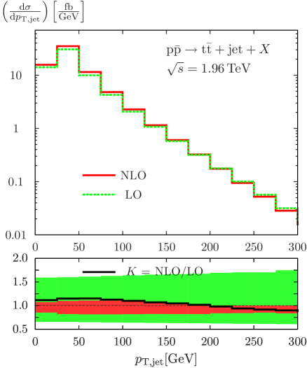
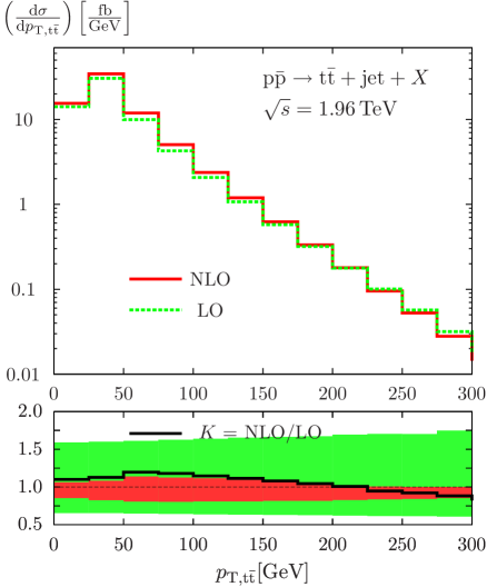
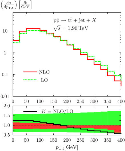
Figure 3.1 shows the distributions in the transverse momenta of the hard jet, $p_{\mathrm{T,jet}}$, of the total ${\mathrm{t}}\bar{\mathrm{t}}$ system, $p_{{\mathrm{T}},{\mathrm{t}}\bar{\mathrm{t}}}$, and of the top-quark, $p_{{\mathrm{T}},{\mathrm{t}}}$.

Figure 3.1: Transverse-momentum distributions of the hard jet ($p_{\mathrm{T,jet}}$), of the total ${\mathrm{t}}\bar{\mathrm{t}}$ system ($p_{{\mathrm{T}},{\mathrm{t}}\bar{\mathrm{t}}}$), and of the top-quark ($p_{{\mathrm{T}},{\mathrm{t}}}$) at the Tevatron. The lower panels show the ratios $K=\mathrm{NLO/LO}$ as well as the LO and NLO scale uncertainties corresponding to a rescaling of $\mu=\mu_{\mathrm{fact}}=\mu_{\mathrm{ren}}=m_{\mathrm{t}}$ by a factor 2.

In LO $p_{\mathrm{T,jet}}$ and $p_{{\mathrm{T}},{\mathrm{t}}\bar{\mathrm{t}}}$ coincide because of momentum conservation in the transverse plane, but the radiation of two jets in the real corrections renders them different. The numerical results in Figure 3.1, however, reveal that the differences are very small. The shown $p_{{\mathrm{T}}}$ distributions drop with growing $p_{{\mathrm{T}}}$, where the spectrum for the top-quark is much harder than the ones for the jet and the ${\mathrm{t}}\bar{\mathrm{t}}$ system. In the $p_{\mathrm{T,jet}}$ and $p_{{\mathrm{T}},{\mathrm{t}}\bar{\mathrm{t}}}$ spectra 93% of the events are concentrated below a $p_{\mathrm{T}}$ of about $100\,\mathrm{GeV}$ at NLO, while 92% of the events have a $p_{{\mathrm{T}},{\mathrm{t}}}$ with less than $200\,\mathrm{GeV}$. Employing a fixed scale $\mu=m_{\mathrm{t}}$, the NLO corrections do not simply rescale the LO shape, but induce distortions at the level of some 10%, which redistribute events from larger to smaller transverse momenta. We believe that two effects contribute to these distorsions. First of all, the use of a fixed renormalization scale $\mu_{\mathrm{ren}}=m_{\mathrm{t}}$ is not an appropriate choice for high $p_{{\mathrm{T}}}$ events. Due to the large value of $\alpha_{\mathrm{s}}$ the LO calculation overestimates the cross section for high $p_{{\mathrm{T}}}$ and the NLO calculation has to compensate this scale choice. We expect that the distortions due to this effect are reduced if an appropriate $p_{{\mathrm{T}}}$-dependent scale choice is used, such as $\mu=\sqrt{p_{{\mathrm{T}}}^{2}+m_{\mathrm{t}}^{2}}$. As a second effect in particular the $p_{{\mathrm{T}}}$ distribution of the top-quarks can become softer due to the emission of additional particles, which is accounted for the first time by an NLO calculation.

As can also be seen from the lower panel of each plot, we find again an important reduction of the scale dependence when the NLO corrections are taken into account. At least for the $p_{\mathrm{T,jet}}$- and $p_{{\mathrm{T}},{\mathrm{t}}\bar{\mathrm{t}}}$-distribution the corrections are of moderate size. For the $p_{{\mathrm{T}},{\mathrm{t}}}$-distribution we find large corrections for large values of $p_{{\mathrm{T}},{\mathrm{t}}}$. The corrections are almost 50% for a $p_{\mathrm{T}}$ arround 400 $\,\mathrm{GeV}$. As mentioned this could probably be cured by employing a $p_{{\mathrm{T}}}$-dependent scale.

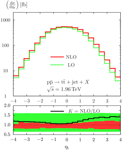
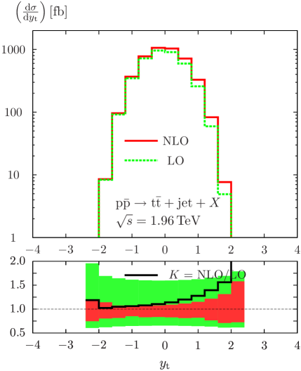
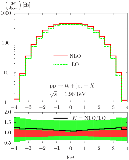
Figure 3.2: Distributions in the pseudo-rapidity ($\eta_{\mathrm{t}}$) and rapidity ($y_{\mathrm{t}}$) of the top-quark, and in the rapidity ($y_{\mathrm{jet}}$) of the hard jet at the Tevatron. The lower panels show the ratios $K=\mathrm{NLO/LO}$ as well as the LO and NLO scale uncertainties corresponding to a rescaling of $\mu=\mu_{\mathrm{fact}}=\mu_{\mathrm{ren}}=m_{\mathrm{t}}$ by a factor 2.

Figure 3.2 depicts the distributions in the pseudo-rapidity and rapidity of the top-quark, $\eta_{\mathrm{t}}$ and $y_{\mathrm{t}}$, and in the rapidity, $y_{\mathrm{jet}}$, of the hard jet. For massless momenta the pseudo-rapidity, which is defined through

$$\eta=-\ln\left(\tan\left({\vartheta\over 2}\right)\right)$$ (3.4)

($\vartheta$ is the scattering angle with respect to the beam axis), is equivalent to the rapidity defined through

$$y={1\over 2}\ln\left({E+p_{z}\over E-p_{z}}\right)$$ (3.5)

($E$ denotes the energy, $p_{z}$ the three-momentum component along the beam axis). For the massive top-quark we observe a rather important difference between the $\eta_{\mathrm{t}}$ and $y_{\mathrm{t}}$ distribution. Recently there has been significant interest in the rapidity distribution of the jet, as MC@NLO [81] and Alpgen with MLM matching [82] disagree on this distribution. Our result includes for the first time the full ${\cal O}(\alpha_{s}^{4})$ matrix elements. Note that the set-up of ref. [82] differs from the one used here, therefore the distributions should not be compared directly.

At NLO, 90% of the events are concentrated within $|\eta_{\mathrm{t}}|<2.0$. Demanding $|y_{\mathrm{t}}|<1.2$ selects 96% of the events. For $y_{\mathrm{jet}}$ we find that 94% of the events are contained in $|y_{\mathrm{jet}}|<2.4$.

The reduction of the forward–backward asymmetry $A^{{\mathrm{t}}}_{\mathrm{FB}}$ discussed above induced by the NLO corrections is clearly visible in the $\eta_{\mathrm{t}}$ and $y_{\mathrm{t}}$ distributions. The corrections are larger in the forward direction. The asymmetry in the LO distributions is thus reduced by the NLO corrections. It is hardly conceivable that this higher-order effect can be absorbed into LO predictions by phase-space-dependent scale choices. It should be realized that the forward–backward-symmetric rapidity distribution of the hard jet gets distorted by the corrections as well. The corrections increase for large values of $|y_{\mathrm{jet}}|$.

At least in the regions of the distributions in which the rate is not too much suppressed, the NLO corrections reduce the scale uncertainty of the LO distributions in a similar way as observed for the integrated cross section.

3.3 Results for the LHC

Table 3.2 shows the integrated cross section for various values of the cut $p_{\mathrm{T,jet,cut}}$ on the transverse momentum of the hard tagging jet at the LHC.

	$\sigma_{{\mathrm{t}}\bar{\mathrm{t}}\mathrm{jet}}[\,\mathrm{pb}]$
$p_{\mathrm{T,jet,cut}}$ [GeV]	LO	NLO
20	710.8(8)${}^{+358}_{-221}$	692(3)3${}^{-40}_{-62}$
50	326.6(4)${}^{+168}_{-103}$	376.2(6)${}^{+17}_{-48}$
100	146.7(2)${}^{+77}_{-47}$	175.0(2)${}^{+10}_{-24}$
200	46.67(6)${}^{+26}_{-15}$	52.81(8)${}^{+0.8}_{-6.7}$

Table 3.2: Cross section $\sigma_{{\mathrm{t}}\bar{\mathrm{t}}\mathrm{jet}}$ at the LHC for different values of $p_{\mathrm{T,jet,cut}}$ for $\mu=\mu_{\mathrm{fact}}=\mu_{\mathrm{ren}}=m_{\mathrm{t}}$. The upper and lower indices are the shifts towards $\mu=m_{\mathrm{t}}/2$ and $\mu=2m_{\mathrm{t}}$.

In contrast to the Tevatron, the ${\mathrm{g}}{\mathrm{g}}$ channel comprises about 70% of the LO ${\mathrm{p}}{\mathrm{p}}$ cross section, followed by $q{\mathrm{g}}$ with about 22% [37]. We note that the importance of the $q{\mathrm{g}}$ channel is very different from the inclusive top-quark production. For inclusive top-quark pair production this channel is suppressed—despite the large parton luminosity in this channel—because it appears only at NLO. For ${\mathrm{t}}\bar{\mathrm{t}}+{\mbox{1-jet}}$ production the $q{\mathrm{g}}$ channel appears already in LO and thus gives a significant contribution due to the large parton luminosity. Comparing the LO and NLO predictions we find again that the large scale dependence of about 100% in the LO cross section is considerably reduced after including the NLO corrections. The ratio of the NLO ${\mathrm{t}}\bar{\mathrm{t}}+{\mbox{1-jet}}$ cross section to the total NLO ${\mathrm{t}}\bar{\mathrm{t}}$ cross section is about 47%, 22%, and 7% for a $p_{\mathrm{T}}$ cut of $50\,\mathrm{GeV}$, $100\,\mathrm{GeV}$, and $200\,\mathrm{GeV}$, respectively.

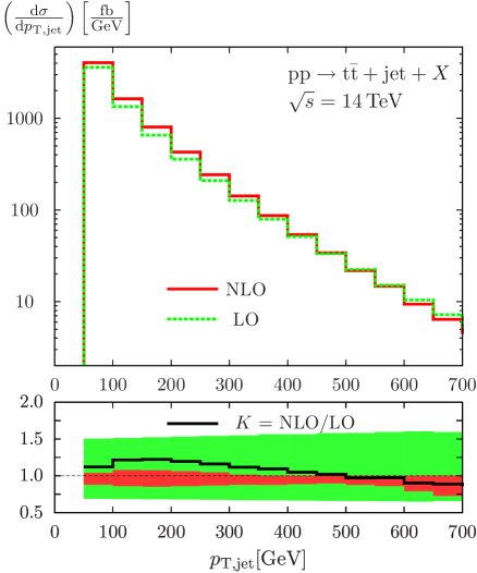
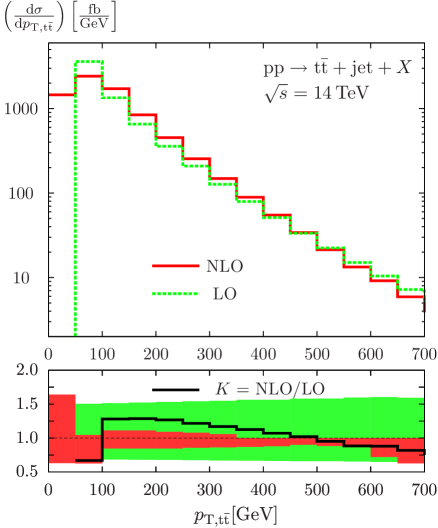
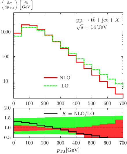
In Figure 3.3 we show the distributions in the transverse momenta of the hard jet, $p_{\mathrm{T,jet}}$, of the total ${\mathrm{t}}\bar{\mathrm{t}}$ system, $p_{{\mathrm{T}},{\mathrm{t}}\bar{\mathrm{t}}}$, and of the top-quark, $p_{{\mathrm{T}},{\mathrm{t}}}$.

Figure 3.3: Transverse-momentum distributions of the hard jet ($p_{\mathrm{T,jet}}$), of the total ${\mathrm{t}}\bar{\mathrm{t}}$ system ($p_{{\mathrm{T}},{\mathrm{t}}\bar{\mathrm{t}}}$), and of the top-quark ($p_{{\mathrm{T}},{\mathrm{t}}}$) at the LHC. The lower panels show the ratios $K=\mathrm{NLO/LO}$ as well as the LO and NLO scale uncertainties corresponding to a rescaling of $\mu=\mu_{\mathrm{fact}}=\mu_{\mathrm{ren}}=m_{\mathrm{t}}$ by a factor 2.

The distributions become harder in $p_{{\mathrm{T}}}$ when going from the Tevatron to the LHC, as expected from the higher scattering energy. At NLO, 92% of the events have transverse momenta $p_{\mathrm{T,jet}}<250\,\mathrm{GeV}$, and 94% have $p_{{\mathrm{T}},{\mathrm{t}}}<300\,\mathrm{GeV}$ in the respective distributions. In contrast to the Tevatron, the $p_{\mathrm{T,jet}}$ and $p_{{\mathrm{T}},{\mathrm{t}}\bar{\mathrm{t}}}$ distributions, which are identical in LO become different in NLO. For the $p_{\mathrm{T,jet}}$-distribution the lowest bin ($0<p_{\mathrm{T,jet}}<50\,\mathrm{GeV}$) is always empty due to the cut applied. For the $p_{{\mathrm{T}},{\mathrm{t}}\bar{\mathrm{t}}}$ this holds also true in LO because the transverse momenta between the ${\mathrm{t}}\bar{\mathrm{t}}$ system and the additional hard jet are balanced. In NLO the lowest bin in the $p_{{\mathrm{T}},{\mathrm{t}}\bar{\mathrm{t}}}$ distribution is populated due to an additional jet. For large $p_{{\mathrm{T}}}$ the difference between $p_{\mathrm{T,jet}}$ and $p_{{\mathrm{T}},{\mathrm{t}}\bar{\mathrm{t}}}$ distributions is at the level of about 10%. This is again due to the presence of the additonal jet. As observed already for the Tevatron, the shapes of the $p_{{\mathrm{T}}}$ distributions receive distortions by the corrections.

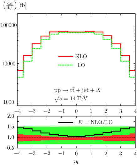
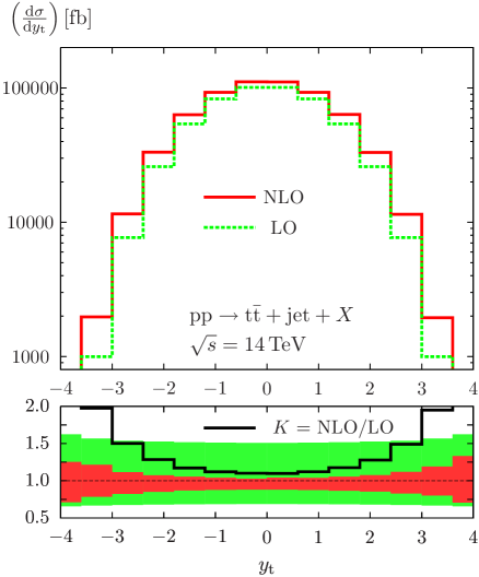
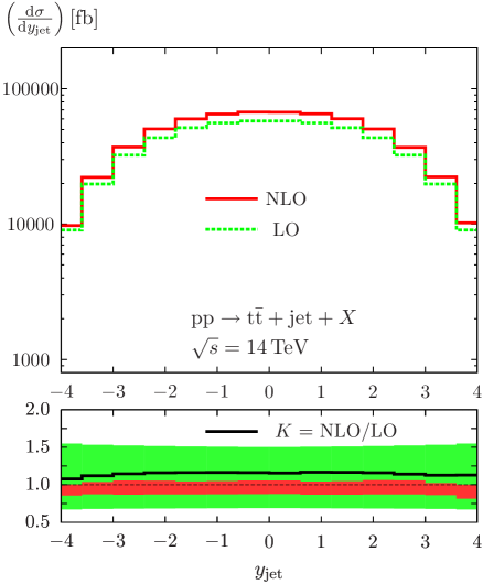
Figure 3.4 illustrates the distributions in the pseudo-rapidity and rapidity of the top-quark, $\eta_{\mathrm{t}}$ and $y_{\mathrm{t}}$, and in the rapidity, $y_{\mathrm{jet}}$, of the hard jet.

Figure 3.4: Distributions in the pseudo-rapidity ($\eta_{\mathrm{t}}$) and rapidity ($y_{\mathrm{t}}$) of the top-quark, and in the rapidity ($y_{\mathrm{jet}}$) of the hard jet at the LHC. The lower panels show the ratios $K=\mathrm{NLO/LO}$ as well as the LO and NLO scale uncertainties corresponding to a rescaling of $\mu=\mu_{\mathrm{fact}}=\mu_{\mathrm{ren}}=m_{\mathrm{t}}$ by a factor 2.

In the respective distributions 92% of the NLO events concentrate within the regions $|\eta_{\mathrm{t}}|<3.0$, 96% have $|y_{\mathrm{t}}|<2.4$, and 96% have $|y_{\mathrm{jet}}|<3.6$ in the respective distributions, i.e. these distributions get broadened roughly by one unit in the transistion from Tevatron to LHC. As for the Tevatron, we find distortions of the shapes induced by the corrections that are hard to mimic by phase-space-dependent scale choices. All the shown $y$ and $\eta$ distributions at the LHC are forward–backward-symmetric, but actually the distributions of top and antitop-quarks are intrinsically different. Numerically we do not observe a significant difference, so that we show only the distributions for the top-quark.

Again, in all shown distributions a reduction of the scale uncertainty by the NLO corrections is visible that is comparable to the one in the integrated cross section.

4 Conclusions

The production of ${\mathrm{t}}\bar{\mathrm{t}}{+}$jet final states represents important processes both at the Tevatron and the LHC. The signal is interesting in its own right, because large fractions of the ${\mathrm{t}}\bar{\mathrm{t}}$ samples show additional jet activity and deviations from the SM could signal new physics such as top-quark compositeness. Moreover, ${\mathrm{t}}\bar{\mathrm{t}}{+}$jet production delivers a large background to many searches at the LHC, such as for the Higgs boson via weak-vector-boson fusion.

We have presented NLO QCD predictions for ${\mathrm{t}}\bar{\mathrm{t}}{+}$jet production at the Tevatron and the LHC. The NLO corrections reduce the scale uncertainty of the total cross section and of the differential distributions compared to a LO calculation, which can only provide qualitative predictions. Further theoretical improvements could only be achieved by dedicated QCD resummations, since a full treatment at NNLO is certainly out of reach. Already the presented NLO calculation is quite complicated. For this reason we have also documented a set of numerical results for the one-loop correction and for the real-emission parts at single phase-space points, in order to facilitate comparisons to our calculation by other groups.

The charge asymmetry of the top-quark, which is measured at the Tevatron, is significantly decreased at NLO and is almost washed out by the residual scale dependence. We have studied the dependence of the NLO asymmetry on the cut on the transverse momentum of the hard tagging jet. Further refinements in the description of the charge asymmetry are required to stabilize the predictions with respect to higher-order corrections. Moreover, the top-quark decay should be taken into account properly.

Finally, the presented NLO QCD calculation for the ${\mathrm{t}}\bar{\mathrm{t}}{+}$jet process represents a building block for a full NNLO QCD prediction for ${\mathrm{t}}\bar{\mathrm{t}}$ production, a demanding and important calculation that is currently in progress by various groups.

Appendix

Appendix A Benchmark numbers for the virtual corrections

In order to facilitate a comparison to our calculation, we provide explicit numbers on the squared LO amplitude and the corresponding virtual corrections for a single non-exceptional phase-space point. The set of momenta for $ab\to{\mathrm{t}}\bar{\mathrm{t}}c$ with the explicit partonic reactions ${\mathrm{g}}{\mathrm{g}}\to{\mathrm{t}}\bar{\mathrm{t}}{\mathrm{g}}$, $q\bar{q}\to{\mathrm{t}}\bar{\mathrm{t}}{\mathrm{g}}$, $q{\mathrm{g}}\to{\mathrm{t}}\bar{\mathrm{t}}q$, and ${\mathrm{g}}\bar{q}\to{\mathrm{t}}\bar{\mathrm{t}}\bar{q}$ is chosen as

$$p_{a} = \scriptstyle(500,0,0,500),$$

$$p_{b} = \scriptstyle(500,0,0,-500),$$

$$p_{{\mathrm{t}}} = \scriptstyle(458.5331753852783,207.0255169909440,0,370.2932732896167),$$

$$p_{\bar{\mathrm{t}}} = \scriptstyle(206.6000026080000,-10.65693677252589,42.52372780926147,-102.3998210421085),$$

$$p_{c} = \scriptstyle(334.8668220067217,-196.3685802184181,-42.52372780926147,-267.8934522475083),$$ (A.1)

with the obvious notation $p=(p^{0},p^{1},p^{2},p^{3})$ and all the components given in GeV. The top-quark mass is set to $m_{\mathrm{t}}=174\,\mathrm{GeV}$. We give numbers on the spin- and colour-averaged squared LO amplitude $|{\cal A}_{5}^{(0)}|^{2}$ as well as for the contribution $2\mathrm{Re}({\cal A}_{5}^{(0)}{{\cal A}_{5}^{(1)}}^{\ast})$. For the Born amplitude we factor out the coupling, we define

$${1\over 4}{1\over{\cal N}_{c}}\sum_{\mbox{\scriptsize spin,colour}}|{\cal A}_{5}^{(0)}|^{2}=g_{\mathrm{s}}^{6}a_{0}.$$ (A.2)

The factor ${1/{\cal N}_{c}}$ is due to the average over the incoming colour. For the channel ${\mathrm{g}}{\mathrm{g}}$, $q\bar{q}$, $q{\mathrm{g}}$, ${\mathrm{g}}\bar{q}$ we have ${\cal N}_{c}=64,$ 9, 24, 24. Note that the coefficient $a_{0}$ only depends on the chosen phase-space point—which implicitly also contains the information about the top-quark mass.

	$a_{0}[\,\mathrm{GeV}^{-2}]$
${\mathrm{g}}{\mathrm{g}}\to{\mathrm{t}}\bar{\mathrm{t}}{\mathrm{g}}$
Version 1	$0.6566843362709776\cdot 10^{-3}$
Version 2	$0.6566843362709785\cdot 10^{-3}$
Madgraph	$0.6566843362709775\cdot 10^{-3}$
$q\bar{q}\to{\mathrm{t}}\bar{\mathrm{t}}{\mathrm{g}}$
Version 1	$0.5790368001550936\cdot 10^{-4}$
Version 2	$0.5790368001550953\cdot 10^{-4}$
Madgraph	$0.5790368001550938\cdot 10^{-4}$
$q{\mathrm{g}}\to{\mathrm{t}}\bar{\mathrm{t}}q$
Version 1	$0.1607845322071585\cdot 10^{-4}$
Version 2	$0.1607845322071587\cdot 10^{-4}$
Madgraph	$0.1607845322071585\cdot 10^{-4}$
${\mathrm{g}}\bar{q}\to{\mathrm{t}}\bar{\mathrm{t}}\bar{q}$
Version 1	$0.2603527972645622\cdot 10^{-3}$
Version 2	$0.2603527972645625\cdot 10^{-3}$
Madgraph	$0.2603527972645620\cdot 10^{-3}$

Table A.1: Colour and spin averaged LO matrix elements squared.

The results for $a_{0}$ are shown in Table A.1. Version 1 and Version 2 correspond to our implementations. For completeness we compare also with Madgraph. The one-loop contribution ${\cal A}^{(1)}$ is renormalised and thus UV finite. However, the virtual corrections still contain collinear and soft singularities. Similar to what has been done in Ref. [54] in a comparison of the virtual corrections to WW+jet production, we use the decomposition

$${1\over 4}{1\over{\cal N}_{c}}\sum_{\mbox{\scriptsize spin,colour}}2\mathrm{Re}({\cal A}_{5}^{(0)}{{\cal A}_{5}^{(1)}}^{\ast})=g_{\mathrm{s}}^{6}a_{0}\,\Gamma(1+\epsilon)\left({4\pi\mu\over m_{\mathrm{t}}^{2}}\right)^{\epsilon}\left(c_{-2}{1\over\epsilon^{2}}+c_{-1}{1\over\epsilon}+c_{0}+{\cal O}(\epsilon)\right).$$ (A.3)

The results are shown in Table A.2. In addition we also give the corresponding results for the I-operator of the dipole subtraction function as defined in Ref. [75], with the auxiliary parameter $\kappa=2/3$. We us the same decomposition as for the one-loop corrections. The individual coefficients are shown in Table A.3. Note that the coefficients $c_{i}$ with $i=-2,-1,0$ contain one factor of $\alpha_{\mathrm{s}}$. We use

$$\alpha_{s}(\mu)=\frac{4\pi}{\beta_{0}L}\left(1-\frac{\beta_{1}}{\beta_{0}^{2}}\frac{\ln L}{L}\right),\;\;\;L=\ln(\mu^{2}/\Lambda^{2}),\;\;\;\beta_{0}=11-\frac{2}{3}N_{f},\;\;\;\beta_{1}=102-\frac{38}{3}N_{f}.$$ (A.4)

with $N_{f}=5$ and $\Lambda=226\,\mathrm{MeV}$, leading to

$$\alpha_{\mathrm{s}}(m_{\mathrm{t}})=0.1075205492734706.$$ (A.5)

	$c_{-2}$	$c_{-1}$	$c_{0}$
${\mathrm{g}}{\mathrm{g}}\to{\mathrm{t}}\bar{\mathrm{t}}{\mathrm{g}}$
Version 1	$-0.1540118420981379$	0.0731096895036588	0.5295183452346090
Version 2	$-0.1540118421074573$	0.0731096894943437	0.5295183452413002
$q\bar{q}\to{\mathrm{t}}\bar{\mathrm{t}}{\mathrm{g}}$
Version 1	$-0.0969704191047176$	$-0.0126983208241891$	0.2435672439083931
Version 2	$-0.0969704191046950$	$-0.0126983208241662$	0.2435672439081981
$q{\mathrm{g}}\to{\mathrm{t}}\bar{\mathrm{t}}q$
Version 1	$-0.0969704191047088$	$-0.0056430956994203$	0.4003849386477017
Version 2	$-0.0969704191046951$	$-0.0056430956994064$	0.4003849386472126
${\mathrm{g}}\bar{q}\to{\mathrm{t}}\bar{\mathrm{t}}\bar{q}$
Version 1	$-0.0969704191046802$	0.0833362739128030	0.5384721403213878
Version 2	$-0.0969704191046950$	0.0833362739127883	0.5384721403213897

Table A.2: Coefficients for colour and spin averaged virtual corrections.

	$c_{-2}$	$c_{-1}$	$c_{0}$
${\mathrm{g}}{\mathrm{g}}\to{\mathrm{t}}\bar{\mathrm{t}}{\mathrm{g}}$
Version 1	0.1540118421074569	$-0.0731096894943435$	$-0.5280576886301999$
Version 2	0.1540118421074573	$-0.0731096894943437$	$-0.5280576886302015$
$q\bar{q}\to{\mathrm{t}}\bar{\mathrm{t}}{\mathrm{g}}$
Version 1	0.0969704191046952	0.0126983208241661	$-0.3992776407671517$
Version 2	0.0969704191046950	0.0126983208241662	$-0.3992776407671513$
$q{\mathrm{g}}\to{\mathrm{t}}\bar{\mathrm{t}}q$
Version 1	0.0969704191046950	0.0056430956994063	$-0.4069645466913195$
Version 2	0.0969704191046951	0.0056430956994064	$-0.4069645466913194$
${\mathrm{g}}\bar{q}\to{\mathrm{t}}\bar{\mathrm{t}}\bar{q}$
Version 1	0.0969704191046950	$-0.0833362739127882$	$-0.3392937280293060$
Version 2	0.0969704191046950	$-0.0833362739127883$	$-0.3392937280293059$

Table A.3: Coefficients for colour and spin averaged results for the I-operator.

For the LO amplitudes we find an agreement of at least 14 digits—pretty close to what one can get using 64bit double precision with 53bits for the mantissa. For the one-loop corrections we find at least an agreement of 10 digits for the finite terms. For the $q\bar{q}$, $q{\mathrm{g}}$, and ${\mathrm{g}}\bar{q}$ channels, which are numerically less involved, we find an agreement of up to 14 digits. The finite terms from the I-operator agree even better. The coefficients of all divergences typically agree to 10 digits, or better in the cases with external quarks. We note, however, that we do not cancel the IR divergences numerically. We also observe a cancellation between the finite part of the I-operator and the corresponding virtual contributions. For the ${\mathrm{g}}{\mathrm{g}}\to{\mathrm{t}}\bar{\mathrm{t}}{\mathrm{g}}$ channel almost three digits are cancelled in the combination.

Appendix B Benchmark numbers for the subtraction terms

In this section we give also results for the subtraction term in the dipole formalism for one phase-space point. We find this useful to facilitate the comparison of upcoming calculations. Recently some effort has been invested to automatize this part of the calculation [83, 84, 85, 86]. The results presented here may provide an interesting benchmark point for these attempts. The set of momenta for $ab\to{\mathrm{t}}\bar{\mathrm{t}}cd$ is chosen as

$$p_{a} = \scriptstyle(2100,-0,-0,2100),$$

$$p_{b} = \scriptstyle(2800,-0,-0,-2800),$$

$$p_{{\mathrm{t}}} = \scriptstyle(1581.118367308447,1254.462316247655,-766.9360998604944,-554.7905976902205),$$

$$p_{\bar{\mathrm{t}}} = \scriptstyle(1460.449317799282,-975.9731477430979,-466.5314749495881,965.6402060944737),$$

$$p_{c} = \scriptstyle(545.4084744819,218.7220720302516,472.0439121434804,-163.7241712507502),$$

$$p_{d} = \scriptstyle(1313.023840410371,-497.2112405348086,761.423662666602,-947.1254371535031),$$ (B.1)

with all components given in GeV. The top-quark mass is set to $m_{\mathrm{t}}=174\,\mathrm{GeV}$. We give numbers on the spin- and colour-averaged squared real emission amplitude $|{\cal A}^{(0)}_{6}|^{2}$ as well as for the sum of the subtraction terms. We define the numbers $b_{0}$ by

$${1\over 4}{1\over{\cal N}_{c}}{1\over{\cal S}}\sum_{\mbox{\scriptsize spin,colour}}|{\cal A}^{(0)}_{6}|^{2}=b_{0}.$$ (B.2)

The factor $1/4$ accounts for the average over the spins of the initial partons, the factor ${1/{\cal N}_{c}}$ is due to the average over the colour of the incoming partons. ${\cal N}_{c}$ contains a factor 8 for every incoming gluon and a factor 3 for every incoming quark or antiquark. ${\cal S}$ is the symmetry factor accounting for identical particles in the final state. The numbers for the dipole subtraction terms are defined analogously:

$${1\over 4}{1\over{\cal S}}\sum\limits_{\mathrm{pairs}\;i,j}\;\sum\limits_{k\neq i,j}{\cal D}_{ij,k}=d_{0}.$$ (B.3)

Note that the factor for the average over the colour of the incoming partons is included in the definition of ${\cal D}_{ij,k}$. The numbers $b_{0}$ and $d_{0}$ contain the strong coupling constant. As numerical value for $\alpha_{\mathrm{s}}$ we use again Eq. (A.4)  with $N_{f}=5$ and $\Lambda=226\,\mathrm{MeV}$, i.e. the value given in Eq. (A.5) .

	$b_{0}[\,\mathrm{GeV}^{-4}]$	$d_{0}[\,\mathrm{GeV}^{-4}]$
${\mathrm{g}}(p_{a}){\mathrm{g}}(p_{b})\to{\mathrm{t}}(p_{{\mathrm{t}}})\bar{\mathrm{t}}(p_{\bar{\mathrm{t}}}){\mathrm{g}}(p_{c}){\mathrm{g}}(p_{d})$
Version 1	$3.12815868347843\cdot 10^{-9}$	$4.1037601540955\cdot 10^{-9}$
Version 2	$3.12815868347842\cdot 10^{-9}$	$4.1037601540962\cdot 10^{-9}$
$q(p_{a})\bar{q}(p_{b})\to{\mathrm{t}}(p_{{\mathrm{t}}})\bar{\mathrm{t}}(p_{\bar{\mathrm{t}}}){\mathrm{g}}(p_{c}){\mathrm{g}}(p_{d})$
Version 1	$4.48308845446477\cdot 10^{-10}$	$4.90476067759639\cdot 10^{-10}$
Version 2	$4.48308845446475\cdot 10^{-10}$	$4.90476067759631\cdot 10^{-10}$
$q(p_{a}){\mathrm{g}}(p_{b})\to{\mathrm{t}}(p_{{\mathrm{t}}})\bar{\mathrm{t}}(p_{\bar{\mathrm{t}}}){\mathrm{g}}(p_{c})q(p_{d})$
Version 1	$1.10256509258713\cdot 10^{-10}$	$1.919073353538\cdot 10^{-10}$
Version 2	$1.10256509258713\cdot 10^{-10}$	$1.919073353539\cdot 10^{-10}$
$\bar{q}(p_{a}){\mathrm{g}}(p_{b})\to{\mathrm{t}}(p_{{\mathrm{t}}})\bar{\mathrm{t}}(p_{\bar{\mathrm{t}}})\bar{q}(p_{c}){\mathrm{g}}(p_{d})$
Version 1	$1.384600673183816\cdot 10^{-10}$	$3.3382231835799\cdot 10^{-10}$
Version 2	$1.384600673183812\cdot 10^{-10}$	$3.3382231835798\cdot 10^{-10}$
${\mathrm{g}}(p_{a}){\mathrm{g}}(p_{b})\to{\mathrm{t}}(p_{{\mathrm{t}}})\bar{\mathrm{t}}(p_{\bar{\mathrm{t}}})\bar{q}(p_{c})q(p_{d})$
Version 1	$2.42841040229558\cdot 10^{-10}$	$4.271065781530\cdot 10^{-10}$
Version 2	$2.42841040229557\cdot 10^{-10}$	$4.271065781532\cdot 10^{-10}$

Table B.1: Colour and spin averaged real emission matrix element squared and dipole subtraction terms related to the processes $0\to{\mathrm{t}}\bar{\mathrm{t}}{\mathrm{g}}{\mathrm{g}}{\mathrm{g}}{\mathrm{g}}$ and $0\to{\mathrm{t}}\bar{\mathrm{t}}q\bar{q}{\mathrm{g}}{\mathrm{g}}$.

	$b_{0}[\,\mathrm{GeV}^{-4}]$	$d_{0}[\,\mathrm{GeV}^{-4}]$
$q(p_{a})q^{\prime}(p_{b})\to{\mathrm{t}}(p_{{\mathrm{t}}})\bar{\mathrm{t}}(p_{\bar{\mathrm{t}}})q^{\prime}(p_{c})q(p_{d})$
Version 1	$4.44137855516180\cdot 10^{-12}$	$1.6381811832266\cdot 10^{-11}$
Version 2	$4.44137855516180\cdot 10^{-12}$	$1.6381811832275\cdot 10^{-11}$
$\bar{q}(p_{a})\bar{q}^{\prime}(p_{b})\to{\mathrm{t}}(p_{{\mathrm{t}}})\bar{\mathrm{t}}(p_{\bar{\mathrm{t}}})\bar{q}(p_{c})\bar{q}^{\prime}(p_{d})$
Version 1	$1.733763330485899\cdot 10^{-11}$	$1.06832579841007\cdot 10^{-10}$
Version 2	$1.733763330485899\cdot 10^{-11}$	$1.06832579841000\cdot 10^{-10}$
$q(p_{a})\bar{q}^{\prime}(p_{b})\to{\mathrm{t}}(p_{{\mathrm{t}}})\bar{\mathrm{t}}(p_{\bar{\mathrm{t}}})\bar{q}^{\prime}(p_{c})q(p_{d})$
Version 1	$4.796260245409952\cdot 10^{-12}$	$1.8776008214791\cdot 10^{-11}$
Version 2	$4.796260245409957\cdot 10^{-12}$	$1.8776008214799\cdot 10^{-11}$
$q(p_{a})\bar{q}(p_{b})\to{\mathrm{t}}(p_{{\mathrm{t}}})\bar{\mathrm{t}}(p_{\bar{\mathrm{t}}})\bar{q}^{\prime}(p_{c})q^{\prime}(p_{d})$
Version 1	$6.13924303047741\cdot 10^{-11}$	$6.990891152615\cdot 10^{-11}$
Version 2	$6.13924303047739\cdot 10^{-11}$	$6.990891152614\cdot 10^{-11}$
$q(p_{a})q(p_{b})\to{\mathrm{t}}(p_{{\mathrm{t}}})\bar{\mathrm{t}}(p_{\bar{\mathrm{t}}})q(p_{c})q(p_{d})$
Version 1	$1.371477814148721\cdot 10^{-11}$	$4.1848434402744\cdot 10^{-11}$
Version 2	$1.371477814148719\cdot 10^{-11}$	$4.1848434402750\cdot 10^{-11}$
$\bar{q}(p_{a})\bar{q}(p_{b})\to{\mathrm{t}}(p_{{\mathrm{t}}})\bar{\mathrm{t}}(p_{\bar{\mathrm{t}}})\bar{q}(p_{c})\bar{q}(p_{d})$
Version 1	$1.411042000289490\cdot 10^{-11}$	$6.3674516988854\cdot 10^{-11}$
Version 2	$1.411042000289488\cdot 10^{-11}$	$6.3674516988857\cdot 10^{-11}$
$q(p_{a})\bar{q}(p_{b})\to{\mathrm{t}}(p_{{\mathrm{t}}})\bar{\mathrm{t}}(p_{\bar{\mathrm{t}}})\bar{q}(p_{c})q(p_{d})$
Version 1	$2.054843839960259\cdot 10^{-11}$	$3.6253236096328\cdot 10^{-11}$
Version 2	$2.054843839960252\cdot 10^{-11}$	$3.6253236096334\cdot 10^{-11}$

Table B.2: Colour and spin averaged real emission matrix element squared and dipole subtraction terms related to the processes $0\to{\mathrm{t}}\bar{\mathrm{t}}q\bar{q}q^{\prime}\bar{q}^{\prime}$ and $0\to{\mathrm{t}}\bar{\mathrm{t}}q\bar{q}q\bar{q}$.

The results for $b_{0}$ and $d_{0}$ are shown in Tables B.1 and B.2. The two implementations agree at least to 14 digits for the matrix elements squared and at least to 12 digits for the sum of the subtraction terms.

Appendix C Tables for histograms

In this appendix we give the tables for the differential distributions. For each distribution, we list the NLO predictions for the scale choice $\mu=m_{\mathrm{t}}/2$, $\mu=m_{\mathrm{t}}$ and $\mu=2m_{\mathrm{t}}$. In all tables we have set $\mu=\mu_{\mathrm{ren}}=\mu_{\mathrm{fact}}$. The errors result from the Monte Carlo integration. The bin is specified by its central value. The bin width—which we chose constant for the entire histogram—is obtained from the distance of two neighboring bin positions. Note that we use the same definition for the cross section as described in Section 3. In particular, we demand a minimum $p_{{\mathrm{T}}}$ for the additional jet. For the Tevatron $20\,\mathrm{GeV}$ is used while for the LHC $50\,\mathrm{GeV}$ is used.

	${\frac{d\sigma}{dp_{{\mathrm{T}},\mathrm{jet}}}}[\frac{\mbox{\scriptsize fb}}{\mbox{\scriptsize GeV}}]$
$p_{{\mathrm{T}},\mathrm{jet}}$ [GeV]	$\mu=m_{\mathrm{t}}/2$	$\mu=m_{\mathrm{t}}$	$\mu=2m_{\mathrm{t}}$
$12.5$	$16.83\pm 0.07$	$15.70\pm 0.04$	$13.4\pm 0.2$
$37.5$	$38.47\pm 0.04$	$35.08\pm 0.03$	$28.83\pm 0.02$
$62.5$	$12.67\pm 0.02$	$11.45\pm 0.01$	$9.340\pm 0.009$
$87.5$	$5.29\pm 0.01$	$4.805\pm 0.008$	$3.92\pm 0.005$
$112.5$	$2.465\pm 0.007$	$2.277\pm 0.006$	$1.864\pm 0.003$
$137.5$	$1.216\pm 0.005$	$1.146\pm 0.003$	$0.943\pm 0.002$
$162.5$	$0.629\pm 0.004$	$0.604\pm 0.002$	$0.496\pm 0.001$
$187.5$	$0.326\pm 0.003$	$0.324\pm 0.002$	$0.2659\pm 0.0007$
$212.5$	$0.173\pm 0.002$	$0.174\pm 0.001$	$0.1460\pm 0.0005$
$237.5$	$0.093\pm 0.001$	$0.0945\pm 0.0008$	$0.0796\pm 0.0004$
$262.5$	$0.047\pm 0.001$	$0.0522\pm 0.0006$	$0.0445\pm 0.0003$
$287.5$	$0.0252\pm 0.0007$	$0.0285\pm 0.0003$	$0.0238\pm 0.0002$
$312.5$	$0.0113\pm 0.0006$	$0.0151\pm 0.0003$	$0.0129\pm 0.0001$

Table C.1: The transverse momentum distribution of the hard jet at the Tevatron.

	${\frac{d\sigma}{dp_{{\mathrm{T}},{\mathrm{t}}\bar{\mathrm{t}}}}}[\frac{\mbox{\scriptsize fb}}{\mbox{\scriptsize GeV}}]$
$p_{{\mathrm{T}},{\mathrm{t}}\bar{\mathrm{t}}}[\mbox{GeV}]$	$\mu=m_{\mathrm{t}}/2$	$\mu=m_{\mathrm{t}}$	$\mu=2m_{\mathrm{t}}$
$12.5$	$16.43\pm 0.07$	$15.49\pm 0.04$	$13.2\pm 0.2$
$37.5$	$37.25\pm 0.05$	$34.43\pm 0.03$	$28.46\pm 0.02$
$62.5$	$13.56\pm 0.02$	$11.91\pm 0.01$	$9.61\pm 0.01$
$87.5$	$5.66\pm 0.01$	$5.036\pm 0.007$	$4.053\pm 0.004$
$112.5$	$2.648\pm 0.007$	$2.373\pm 0.005$	$1.919\pm 0.003$
$137.5$	$1.309\pm 0.006$	$1.194\pm 0.003$	$0.967\pm 0.002$
$162.5$	$0.669\pm 0.004$	$0.623\pm 0.002$	$0.509\pm 0.001$
$187.5$	$0.345\pm 0.002$	$0.332\pm 0.001$	$0.2720\pm 0.0007$
$212.5$	$0.180\pm 0.002$	$0.1791\pm 0.0008$	$0.1482\pm 0.0005$
$237.5$	$0.096\pm 0.001$	$0.0953\pm 0.0006$	$0.0797\pm 0.0004$
$262.5$	$0.0466\pm 0.0009$	$0.0525\pm 0.0005$	$0.0443\pm 0.0002$
$287.5$	$0.0243\pm 0.0007$	$0.0280\pm 0.0003$	$0.0239\pm 0.0002$
$312.5$	$0.0113\pm 0.0005$	$0.0144\pm 0.0003$	$0.0126\pm 0.0001$

Table C.2: The transverse momentum distribution of the total ${\mathrm{t}}\bar{\mathrm{t}}$ system at the Tevatron.

	${\frac{d\sigma}{dp_{{\mathrm{T}},{\mathrm{t}}}}}[\frac{\mbox{\scriptsize fb}}{\mbox{\scriptsize GeV}}]$
$p_{{\mathrm{T}},{\mathrm{t}}}[\mbox{GeV}]$	$\mu=m_{\mathrm{t}}/2$	$\mu=m_{\mathrm{t}}$	$\mu=2m_{\mathrm{t}}$
$12.5$	$4.12\pm 0.02$	$3.58\pm 0.01$	$2.910\pm 0.007$
$37.5$	$10.96\pm 0.03$	$9.62\pm 0.02$	$7.78\pm 0.02$
$62.5$	$14.31\pm 0.03$	$12.68\pm 0.02$	$10.35\pm 0.02$
$87.5$	$14.11\pm 0.03$	$12.63\pm 0.02$	$10.58\pm 0.02$
$112.5$	$11.67\pm 0.03$	$10.66\pm 0.02$	$8.72\pm 0.01$
$137.5$	$8.53\pm 0.02$	$7.94\pm 0.01$	$6.59\pm 0.01$
$162.5$	$5.75\pm 0.02$	$5.48\pm 0.01$	$4.570\pm 0.008$
$187.5$	$3.59\pm 0.03$	$3.59\pm 0.01$	$3.019\pm 0.008$
$212.5$	$2.23\pm 0.02$	$2.24\pm 0.01$	$1.923\pm 0.006$
$237.5$	$1.30\pm 0.01$	$1.391\pm 0.008$	$1.189\pm 0.004$
$262.5$	$0.76\pm 0.01$	$0.837\pm 0.006$	$0.721\pm 0.004$
$287.5$	$0.43\pm 0.01$	$0.488\pm 0.004$	$0.428\pm 0.003$
$312.5$	$0.237\pm 0.009$	$0.286\pm 0.004$	$0.254\pm 0.003$
$337.5$	$0.139\pm 0.006$	$0.167\pm 0.003$	$0.146\pm 0.002$
$362.5$	$0.067\pm 0.005$	$0.088\pm 0.003$	$0.082\pm 0.002$
$387.5$	$0.032\pm 0.005$	$0.051\pm 0.002$	$0.047\pm 0.001$

Table C.3: The transverse momentum distribution of the top-quark at the Tevatron.

	${\frac{d\sigma}{d\eta_{{\mathrm{t}}}}}[\mbox{fb}]$
$\eta_{{\mathrm{t}}}$	$\mu=m_{\mathrm{t}}/2$	$\mu=m_{\mathrm{t}}$	$\mu=2m_{\mathrm{t}}$
$-3.8$	$6.6\pm 0.2$	$6.3\pm 0.1$	$5.2\pm 0.1$
$-3.4$	$16.0\pm 0.3$	$13.7\pm 0.2$	$11.2\pm 0.1$
$-3.0$	$33.5\pm 0.4$	$30.1\pm 0.3$	$24.1\pm 0.2$
$-2.6$	$70.1\pm 0.8$	$62.5\pm 0.3$	$50.9\pm 0.2$
$-2.2$	$136.4\pm 0.8$	$123.3\pm 0.5$	$100.3\pm 0.3$
$-1.8$	$237\pm 1$	$219.6\pm 0.9$	$188\pm 9$
$-1.4$	$363\pm 1$	$338.1\pm 0.8$	$279.6\pm 0.5$
$-1.0$	$483\pm 1$	$451.8\pm 0.8$	$376.2\pm 0.6$
$-0.6$	$546\pm 2$	$519\pm 1$	$437\pm 2$
$-0.2$	$573\pm 2$	$543.8\pm 0.9$	$454.5\pm 0.6$
$0.2$	$573\pm 2$	$534.3\pm 0.8$	$446.2\pm 0.6$
$0.6$	$542\pm 1$	$496.6\pm 0.9$	$409.1\pm 0.6$
$1.0$	$467\pm 1$	$420.7\pm 0.8$	$341.4\pm 0.6$
$1.4$	$354\pm 1$	$310\pm 1$	$248.6\pm 0.5$
$1.8$	$229\pm 1$	$197.2\pm 0.5$	$165\pm 9$
$2.2$	$130.5\pm 0.7$	$109.4\pm 0.4$	$86.4\pm 0.3$
$2.6$	$65.9\pm 0.5$	$55.3\pm 0.3$	$43.0\pm 0.2$
$3.0$	$32.4\pm 0.4$	$26.6\pm 0.2$	$20.9\pm 0.2$
$3.4$	$15.2\pm 0.3$	$12.4\pm 0.1$	$9.7\pm 0.1$
$3.8$	$6.7\pm 0.2$	$5.7\pm 0.1$	$4.42\pm 0.08$

Table C.4: The pseudo-rapidity distribution of the top-quark at the Tevatron.

	${\frac{d\sigma}{dy_{{\mathrm{t}}}}}[\mbox{fb}]$
$y_{{\mathrm{t}}}$	$\mu=m_{\mathrm{t}}/2$	$\mu=m_{\mathrm{t}}$	$\mu=2m_{\mathrm{t}}$
$-1.8$	$9.8\pm 0.3$	$8.5\pm 0.1$	$6.9\pm 0.1$
$-1.4$	$103.5\pm 0.8$	$96.3\pm 0.4$	$78.5\pm 0.3$
$-1.0$	$388\pm 1$	$368.4\pm 0.8$	$314\pm 9$
$-0.6$	$826\pm 2$	$777\pm 2$	$645.0\pm 0.8$
$-0.2$	$1144\pm 2$	$1063\pm 1$	$888\pm 2$
$0.2$	$1131\pm 3$	$1035\pm 1$	$856.6\pm 0.8$
$0.6$	$799\pm 2$	$716\pm 1$	$581.9\pm 0.8$
$1.0$	$379\pm 1$	$329.4\pm 0.9$	$270\pm 9$
$1.4$	$100.9\pm 0.6$	$82.9\pm 0.3$	$63.5\pm 0.2$
$1.8$	$10.1\pm 0.1$	$7.68\pm 0.08$	$5.46\pm 0.07$

Table C.5: The rapidity distribution of the top-quark at the Tevatron.

	${\frac{d\sigma}{dy_{\mathrm{jet}}}}[\mbox{fb}]$
$y_{\mathrm{jet}}$	$\mu=m_{\mathrm{t}}/2$	$\mu=m_{\mathrm{t}}$	$\mu=2m_{\mathrm{t}}$
$-3.8$	$1.5\pm 0.1$	$1.26\pm 0.09$	$1.0\pm 0.1$
$-3.4$	$10.8\pm 0.4$	$9.4\pm 0.2$	$7.5\pm 0.2$
$-3.0$	$41.1\pm 0.7$	$35.8\pm 0.4$	$28.5\pm 0.3$
$-2.6$	$100\pm 1$	$88.0\pm 0.6$	$70.3\pm 0.4$
$-2.2$	$192\pm 1$	$168.2\pm 0.7$	$135.0\pm 0.5$
$-1.8$	$295\pm 1$	$266\pm 1$	$215.5\pm 0.6$
$-1.4$	$397\pm 2$	$357\pm 1$	$293.3\pm 0.6$
$-1.0$	$456\pm 2$	$422\pm 1$	$348.4\pm 0.6$
$-0.6$	$481\pm 2$	$447\pm 1$	$380\pm 9$
$-0.2$	$471\pm 2$	$449\pm 2$	$374.4\pm 0.7$
$0.2$	$475\pm 2$	$448\pm 2$	$374.9\pm 0.7$
$0.6$	$477\pm 2$	$445\pm 2$	$380\pm 9$
$1.0$	$457\pm 2$	$421\pm 1$	$348.8\pm 0.5$
$1.4$	$396\pm 2$	$359\pm 1$	$292.8\pm 0.5$
$1.8$	$294\pm 1$	$265\pm 1$	$214.9\pm 0.5$
$2.2$	$191\pm 2$	$167.9\pm 0.6$	$135.3\pm 0.5$
$2.6$	$101.1\pm 0.9$	$89.0\pm 0.5$	$70.1\pm 0.4$
$3.0$	$41.8\pm 0.6$	$36.1\pm 0.4$	$28.7\pm 0.3$
$3.4$	$11.3\pm 0.3$	$9.8\pm 0.2$	$7.7\pm 0.2$
$3.8$	$1.5\pm 0.1$	$1.16\pm 0.09$	$0.92\pm 0.07$

Table C.6: The rapidity distribution of the hard jet at the Tevatron.

	${\frac{d\sigma}{dp_{{\mathrm{T}},\mathrm{jet}}}}[\frac{\mbox{\scriptsize fb}}{\mbox{\scriptsize GeV}}]$
$p_{{\mathrm{T}},\mathrm{jet}}[\mbox{GeV}]$	$\mu=m_{\mathrm{t}}/2$	$\mu=m_{\mathrm{t}}$	$\mu=2m_{\mathrm{t}}$
$25$	$0$	$0$	$0$
$75$	$4201\pm 11$	$4045\pm 5$	$3553\pm 4$
$125$	$1762\pm 5$	$1635\pm 2$	$1405\pm 2$
$175$	$863\pm 3$	$802\pm 2$	$685\pm 1$
$225$	$454\pm 3$	$428\pm 1$	$368.0\pm 0.8$
$275$	$254\pm 2$	$242.7\pm 0.7$	$210.9\pm 0.5$
$325$	$144\pm 1$	$142.1\pm 0.5$	$124.9\pm 0.4$
$375$	$85.9\pm 0.7$	$86.8\pm 0.4$	$76.2\pm 0.3$
$425$	$51.5\pm 0.5$	$53.8\pm 0.3$	$47.7\pm 0.2$
$475$	$31.3\pm 0.6$	$34.1\pm 0.2$	$30.6\pm 0.1$
$525$	$19.1\pm 0.5$	$21.8\pm 0.3$	$20.0\pm 0.1$
$575$	$12.6\pm 0.2$	$14.7\pm 0.2$	$13.01\pm 0.08$
$625$	$7.4\pm 0.2$	$9.4\pm 0.1$	$9.06\pm 0.06$
$675$	$4.7\pm 0.1$	$6.40\pm 0.09$	$6.07\pm 0.05$

Table C.7: The transverse momentum distribution of the hard jet at the LHC.

	${\frac{d\sigma}{dp_{{\mathrm{T}},{\mathrm{t}}\bar{\mathrm{t}}}}}[\frac{\mbox{\scriptsize fb}}{\mbox{\scriptsize GeV}}]$
$p_{{\mathrm{T}},{\mathrm{t}}\bar{\mathrm{t}}}[\mbox{GeV}]$	$\mu=m_{\mathrm{t}}/2$	$\mu=m_{\mathrm{t}}$	$\mu=2m_{\mathrm{t}}$
$25$	$2390\pm 10$	$1457\pm 6$	$920\pm 2$
$75$	$1512\pm 11$	$2418\pm 5$	$2524\pm 4$
$125$	$1915\pm 5$	$1722\pm 3$	$1460\pm 1$
$175$	$938\pm 3$	$843\pm 2$	$714\pm 1$
$225$	$496\pm 2$	$454\pm 1$	$383.9\pm 0.7$
$275$	$274\pm 1$	$254.4\pm 0.7$	$217.9\pm 0.5$
$325$	$157\pm 1$	$148.7\pm 0.5$	$128.2\pm 0.4$
$375$	$88\pm 1$	$89.2\pm 0.4$	$77.7\pm 0.3$
$425$	$54.5\pm 0.8$	$54.9\pm 0.3$	$48.3\pm 0.2$
$475$	$31.6\pm 0.6$	$34.1\pm 0.2$	$30.7\pm 0.2$
$525$	$18.8\pm 0.6$	$21.4\pm 0.2$	$19.8\pm 0.1$
$575$	$11.5\pm 0.2$	$13.3\pm 0.2$	$13.07\pm 0.09$
$625$	$6.6\pm 0.2$	$9.2\pm 0.2$	$8.50\pm 0.08$
$675$	$3.7\pm 0.1$	$5.91\pm 0.07$	$5.72\pm 0.06$

Table C.8: The transverse momentum distribution of the total ${\mathrm{t}}\bar{\mathrm{t}}$ system at the LHC.

	${\frac{d\sigma}{dp_{{\mathrm{T}},{\mathrm{t}}}}}[\frac{\mbox{\scriptsize fb}}{\mbox{\scriptsize GeV}}]$
$p_{{\mathrm{T}},{\mathrm{t}}}[\mbox{GeV}]$	$\mu=m_{\mathrm{t}}/2$	$\mu=m_{\mathrm{t}}$	$\mu=2m_{\mathrm{t}}$
$25$	$995\pm 3$	$881\pm 2$	$740\pm 2$
$75$	$2152\pm 5$	$1930\pm 4$	$1639\pm 2$
$125$	$2029\pm 6$	$1858\pm 3$	$1597\pm 3$
$175$	$1338\pm 11$	$1276\pm 2$	$1115\pm 2$
$225$	$723\pm 7$	$744\pm 2$	$662\pm 2$
$275$	$368\pm 2$	$400\pm 1$	$365.8\pm 0.9$
$325$	$178\pm 2$	$209.3\pm 0.8$	$196.4\pm 0.5$
$375$	$83\pm 1$	$110.5\pm 0.6$	$107.5\pm 0.6$
$425$	$37.9\pm 0.7$	$58.4\pm 0.4$	$60.1\pm 0.5$
$475$	$14.9\pm 0.6$	$31.8\pm 0.3$	$33.8\pm 0.2$
$525$	$4.5\pm 0.4$	$17.5\pm 0.2$	$19.6\pm 0.1$
$575$	$0.1\pm 0.3$	$9.6\pm 0.2$	$11.4\pm 0.2$
$625$	–	$5.4\pm 0.1$	$6.6\pm 0.1$
$675$	–	$3.0\pm 0.1$	$4.21\pm 0.07$

Table C.9: The transverse momentum distribution of the top-quark at the LHC.

	${\frac{d\sigma}{d\eta_{{\mathrm{t}}}}}[\mbox{pb}]$
$\eta_{{\mathrm{t}}}$	$\mu=m_{\mathrm{t}}/2$	$\mu=m_{\mathrm{t}}$	$\mu=2m_{\mathrm{t}}$
$-5.7$	$0.27\pm 0.04$	$0.21\pm 0.01$	$0.184\pm 0.008$
$-5.1$	$0.85\pm 0.04$	$0.71\pm 0.03$	$0.58\pm 0.01$
$-4.5$	$2.58\pm 0.07$	$2.27\pm 0.03$	$1.92\pm 0.04$
$-3.9$	$7.5\pm 0.1$	$6.55\pm 0.05$	$5.35\pm 0.05$
$-3.3$	$18.3\pm 0.1$	$16.3\pm 0.1$	$13.54\pm 0.07$
$-2.7$	$36.4\pm 0.2$	$32.8\pm 0.1$	$27.86\pm 0.07$
$-2.1$	$56.1\pm 0.2$	$52.2\pm 0.1$	$45.05\pm 0.09$
$-1.5$	$69.6\pm 0.2$	$66.7\pm 0.2$	$58.3\pm 0.1$
$-0.9$	$70.4\pm 0.5$	$69.7\pm 0.1$	$61.64\pm 0.09$
$-0.3$	$66.6\pm 0.2$	$66.7\pm 0.1$	$59.28\pm 0.09$
$0.3$	$67.0\pm 0.2$	$66.5\pm 0.1$	$59.39\pm 0.09$
$0.9$	$71.4\pm 0.3$	$69.5\pm 0.3$	$61.57\pm 0.09$
$1.5$	$69.6\pm 0.2$	$66.6\pm 0.3$	$58.1\pm 0.1$
$2.1$	$56.3\pm 0.3$	$52.8\pm 0.3$	$45.10\pm 0.08$
$2.7$	$36.0\pm 0.2$	$32.6\pm 0.2$	$27.80\pm 0.08$
$3.3$	$18.3\pm 0.1$	$16.3\pm 0.1$	$13.43\pm 0.08$
$3.9$	$7.8\pm 0.2$	$6.57\pm 0.05$	$5.43\pm 0.04$
$4.5$	$2.6\pm 0.1$	$2.28\pm 0.04$	$1.82\pm 0.03$
$5.1$	$0.83\pm 0.04$	$0.70\pm 0.02$	$0.61\pm 0.01$
$5.7$	$0.25\pm 0.02$	$0.20\pm 0.01$	$0.171\pm 0.009$

Table C.10: The pseudo-rapidity distribution of the top-quark at the LHC.

	${\frac{d\sigma}{dy_{{\mathrm{t}}}}}[\mbox{pb}]$
$y_{{\mathrm{t}}}$	$\mu=m_{\mathrm{t}}/2$	$\mu=m_{\mathrm{t}}$	$\mu=2m_{\mathrm{t}}$
$-3.9$	$0.093\pm 0.008$	$0.075\pm 0.006$	$0.053\pm 0.004$
$-3.3$	$2.39\pm 0.06$	$1.97\pm 0.04$	$1.55\pm 0.02$
$-2.7$	$12.9\pm 0.1$	$11.55\pm 0.09$	$9.52\pm 0.05$
$-2.1$	$35.7\pm 0.2$	$33.3\pm 0.1$	$28.35\pm 0.07$
$-1.5$	$66.7\pm 0.2$	$63.3\pm 0.2$	$55.1\pm 0.1$
$-0.9$	$96.5\pm 0.3$	$92.9\pm 0.2$	$81.5\pm 0.1$
$-0.3$	$114.1\pm 0.6$	$111.1\pm 0.2$	$97.7\pm 0.1$
$0.3$	$115.6\pm 0.3$	$110.9\pm 0.2$	$97.7\pm 0.1$
$0.9$	$96.5\pm 0.2$	$92.9\pm 0.2$	$81.4\pm 0.2$
$1.5$	$67.0\pm 0.3$	$63.5\pm 0.2$	$55.0\pm 0.1$
$2.1$	$35.6\pm 0.2$	$33.1\pm 0.1$	$28.32\pm 0.07$
$2.7$	$12.8\pm 0.1$	$11.45\pm 0.07$	$9.50\pm 0.06$
$3.3$	$2.32\pm 0.08$	$1.95\pm 0.03$	$1.56\pm 0.02$
$3.9$	$0.095\pm 0.006$	$0.071\pm 0.005$	$0.050\pm 0.003$

Table C.11: The rapidity distribution of the top-quark at the LHC.

	${\frac{d\sigma}{dy_{\mathrm{jet}}}}[\mbox{pb}]$
$y_{\mathrm{jet}}$	$\mu=m_{\mathrm{t}}/2$	$\mu=m_{\mathrm{t}}$	$\mu=2m_{\mathrm{t}}$
$-5.1$	$0.05\pm 0.04$	$0.18\pm 0.02$	$0.12\pm 0.01$
$-4.5$	$2.2\pm 0.1$	$2.09\pm 0.07$	$1.88\pm 0.04$
$-3.9$	$9.8\pm 0.2$	$9.8\pm 0.1$	$8.34\pm 0.07$
$-3.3$	$23.0\pm 0.2$	$22.2\pm 0.1$	$19.38\pm 0.08$
$-2.7$	$39.1\pm 0.3$	$37.1\pm 0.1$	$32.21\pm 0.08$
$-2.1$	$53.3\pm 0.5$	$50.5\pm 0.1$	$44.01\pm 0.09$
$-1.5$	$62.6\pm 0.5$	$59.9\pm 0.2$	$52.2\pm 0.1$
$-0.9$	$68.3\pm 0.6$	$65.1\pm 0.2$	$56.8\pm 0.1$
$-0.3$	$71.1\pm 0.3$	$67.2\pm 0.1$	$58.8\pm 0.1$
$0.3$	$70.7\pm 0.3$	$67.0\pm 0.3$	$58.8\pm 0.1$
$0.9$	$68.1\pm 0.3$	$65.4\pm 0.3$	$56.8\pm 0.2$
$1.5$	$63.0\pm 0.3$	$60.1\pm 0.1$	$52.1\pm 0.1$
$2.1$	$53.6\pm 0.3$	$50.5\pm 0.1$	$44.0\pm 0.1$
$2.7$	$39.1\pm 0.3$	$36.9\pm 0.1$	$32.18\pm 0.09$
$3.3$	$22.8\pm 0.2$	$22.3\pm 0.1$	$19.3\pm 0.1$
$3.9$	$9.9\pm 0.1$	$10.2\pm 0.4$	$8.34\pm 0.06$
$4.5$	$2.09\pm 0.09$	$2.2\pm 0.1$	$1.88\pm 0.06$
$5.1$	$0.12\pm 0.02$	$0.13\pm 0.02$	$0.12\pm 0.01$

Table C.12: The rapidity distribution of the hard jet at the LHC.

References

• [1] CDF - Run II and D0 - Run II, U. Heintz, (2008), arXiv:0806.1202.
• [2] W. Bernreuther, J. Phys. G35, 083001 (2008), arXiv:0805.1333.
• [3] T. Han, (2008), arXiv:0804.3178.
• [4] E. Vanes, Plenary Talk at ICHEP 08, Philadelphia, USA, Jul. 29th - Aug. 5th, 2008.
• [5] D0, V. M. Abazov et al., Phys. Rev. Lett. 98, 181802 (2007), hep-ex/0612052.
• [6] D0, V. M. Abazov et al., Phys. Rev. D78, 012005 (2008), arXiv:0803.0739.
• [7] CDF, T. Aaltonen et al., (2008), arXiv:0809.2581.
• [8] B. W. Harris, E. Laenen, L. Phaf, Z. Sullivan, and S. Weinzierl, Phys. Rev. D66, 054024 (2002), hep-ph/0207055.
• [9] Z. Sullivan, Phys. Rev. D70, 114012 (2004), hep-ph/0408049.
• [10] N. Kidonakis, Phys. Rev. D74, 114012 (2006), hep-ph/0609287.
• [11] N. Kidonakis, Phys. Rev. D75, 071501 (2007), hep-ph/0701080.
• [12] CDF, A. A. Affolder et al., Phys. Rev. Lett. 84, 216 (2000), hep-ex/9909042.
• [13] CDF, D. E. Acosta et al., Phys. Rev. D71, 031101 (2005), hep-ex/0411070.
• [14] CDF, A. Abulencia et al., Phys. Rev. D73, 111103 (2006), hep-ex/0511023.
• [15] CDF II, A. Abulencia et al., Phys. Rev. D75, 052001 (2007), hep-ex/0612011.
• [16] D0, V. M. Abazov et al., Phys. Rev. Lett. 100, 062004 (2008), arXiv:0711.0032.
• [17] D0, V. M. Abazov et al., Phys. Rev. D75, 031102 (2007), hep-ex/0609045.
• [18] D0, V. M. Abazov et al., Phys. Lett. B617, 1 (2005), hep-ex/0404040.
• [19] W. Bernreuther, A. Brandenburg, Z. G. Si, and P. Uwer, Phys. Rev. Lett. 87, 242002 (2001), hep-ph/0107086.
• [20] W. Bernreuther, A. Brandenburg, Z. G. Si, and P. Uwer, Nucl. Phys. B690, 81 (2004), hep-ph/0403035.
• [21] A. Lazopoulos, T. McElmurry, K. Melnikov, and F. Petriello, (2008), arXiv:0804.2220.
• [22] W. Beenakker et al., Phys. Rev. Lett. 87, 201805 (2001), hep-ph/0107081.
• [23] W. Beenakker et al., Nucl. Phys. B653, 151 (2003), hep-ph/0211352.
• [24] S. Dawson, L. H. Orr, L. Reina, and D. Wackeroth, Phys. Rev. D67, 071503 (2003), hep-ph/0211438.
• [25] S. Dawson, C. Jackson, L. H. Orr, L. Reina, and D. Wackeroth, Phys. Rev. D68, 034022 (2003), hep-ph/0305087.
• [26] S. Moch and P. Uwer, (2008), arXiv:0804.1476.
• [27] F. Halzen, P. Hoyer, and C. S. Kim, Phys. Lett. B195, 74 (1987).
• [28] J. H. Kühn and G. Rodrigo, Phys. Rev. D59, 054017 (1999), hep-ph/9807420.
• [29] J. H. Kühn and G. Rodrigo, Phys. Rev. Lett. 81, 49 (1998), hep-ph/9802268.
• [30] M. T. Bowen, S. D. Ellis, and D. Rainwater, Phys. Rev. D73, 014008 (2006), hep-ph/0509267.
• [31] F. A. Berends, K. J. F. Gaemers, and R. Gastmans, Nucl. Phys. B63, 381 (1973).
• [32] F. A. Berends, R. Kleiss, S. Jadach, and Z. Was, Acta Phys. Polon. B14, 413 (1983).
• [33] D0, V. M. Abazov et al., Phys. Rev. Lett. 100, 142002 (2008), 0712.0851.
• [34] CDF, T. Aaltonen et al., (2008), arXiv:0806.2472.
• [35] O. Antunano, J. H. Kühn, and G. Rodrigo, Phys. Rev. D77, 014003 (2008), arXiv:0709.1652.
• [36] L. G. Almeida, G. Sterman, and W. Vogelsang, Phys. Rev. D78, 014008 (2008), arXiv:0805.1885.
• [37] S. Dittmaier, P. Uwer, and S. Weinzierl, Phys. Rev. Lett. 98, 262002 (2007), hep-ph/0703120.
• [38] M. Cacciari, S. Frixione, M. M. Mangano, P. Nason, and G. Ridolfi, (2008), arXiv:0804.2800.
• [39] N. Kidonakis and R. Vogt, (2008), arXiv:0805.3844.
• [40] J. G. Körner, Z. Merebashvili, and M. Rogal, Phys. Rev. D73, 034030 (2006), hep-ph/0511264.
• [41] J. G. Körner, Z. Merebashvili, and M. Rogal, Phys. Rev. D77, 094011 (2008), arXiv:0802.0106.
• [42] S. Moch and A. Mitov, Acta Phys. Polon. B38, 3507 (2007), arXiv:0711.1121.
• [43] M. Czakon, A. Mitov, and S. Moch, Phys. Lett. B651, 147 (2007), 0705.1975.
• [44] M. Czakon, A. Mitov, and S. Moch, Nucl. Phys. B798, 210 (2008), arXiv:0707.4139.
• [45] M. Czakon, Phys. Lett. B664, 307 (2008), arXiv:0803.1400.
• [46] R. Bonciani, A. Ferroglia, T. Gehrmann, D. Maitre, and C. Studerus, (2008), arXiv:0806.2301.
• [47] C. Anastasiou and S. M. Aybat, (2008), arXiv:0809.1355.
• [48] B. Kniehl, J. G. Korner, Z. Merebashvili, and M. Rogal, (2008), arXiv:0809.3980.
• [49] R. K. Ellis, W. T. Giele, Z. Kunszt, and K. Melnikov, (2008), arXiv:0806.3467.
• [50] S. Asai et al., Eur. Phys. J. C32S2, 19 (2004), hep-ph/0402254.
• [51] S. Abdullin et al., Eur. Phys. J. C39S2, 41 (2005).
• [52] A. Alves, O. Eboli, T. Plehn, and D. L. Rainwater, Phys. Rev. D69, 075005 (2004), hep-ph/0309042.
• [53] C. Buttar et al., (2006), hep-ph/0604120.
• [54] NLO Multileg Working Group, Z. Bern et al., (2008), arXiv:0803.0494.
• [55] T. Stelzer and W. F. Long, Comput. Phys. Commun. 81, 357 (1994), hep-ph/9401258.
• [56] J. Küblbeck, M. Böhm, and A. Denner, Comput. Phys. Commun. 60, 165 (1990).
• [57] T. Hahn, Comput. Phys. Commun. 140, 418 (2001), hep-ph/0012260.
• [58] S. Dittmaier, Nucl. Phys. B675, 447 (2003), hep-ph/0308246.
• [59] A. Bredenstein, A. Denner, S. Dittmaier, and S. Pozzorini, JHEP 08, 108 (2008), arXiv:0807.1248.
• [60] A. Denner and S. Dittmaier, Nucl. Phys. B658, 175 (2003), hep-ph/0212259.
• [61] T. Binoth, J. P. Guillet, G. Heinrich, E. Pilon, and C. Schubert, JHEP 10, 015 (2005), hep-ph/0504267.
• [62] G. Passarino and M. J. G. Veltman, Nucl. Phys. B160, 151 (1979).
• [63] G. ’t Hooft and M. J. G. Veltman, Nucl. Phys. B153, 365 (1979).
• [64] W. Beenakker and A. Denner, Nucl. Phys. B338, 349 (1990).
• [65] A. Denner, U. Nierste, and R. Scharf, Nucl. Phys. B367, 637 (1991).
• [66] A. Denner and S. Dittmaier, Nucl. Phys. B734, 62 (2006), hep-ph/0509141.
• [67] P. Nogueira, J. Comput. Phys. 105, 279 (1993).
• [68] J. A. M. Vermaseren, (2000), math-ph/0010025.
• [69] W. T. Giele and E. W. N. Glover, JHEP 04, 029 (2004), hep-ph/0402152.
• [70] G. J. van Oldenborgh and J. A. M. Vermaseren, Z. Phys. C46, 425 (1990).
• [71] G. J. van Oldenborgh, Comput. Phys. Commun. 66, 1 (1991).
• [72] W. Giele, E. W. N. Glover, and G. Zanderighi, Nucl. Phys. Proc. Suppl. 135, 275 (2004), hep-ph/0407016.
• [73] S. Catani and M. H. Seymour, Nucl. Phys. B485, 291 (1997), hep-ph/9605323.
• [74] L. Phaf and S. Weinzierl, JHEP 04, 006 (2001), hep-ph/0102207.
• [75] S. Catani, S. Dittmaier, M. H. Seymour, and Z. Trócsańyi, Nucl. Phys. B627, 189 (2002), hep-ph/0201036.
• [76] S. Weinzierl, Eur. Phys. J. C45, 745 (2006), hep-ph/0510157.
• [77] F. A. Berends and W. T. Giele, Nucl. Phys. B306, 759 (1988).
• [78] S. Weinzierl and D. A. Kosower, Phys. Rev. D60, 054028 (1999), hep-ph/9901277.
• [79] J. Pumplin et al., JHEP 07, 012 (2002), hep-ph/0201195.
• [80] S. D. Ellis and D. E. Soper, Phys. Rev. D48, 3160 (1993), hep-ph/9305266.
• [81] S. Frixione, P. Nason, and B. R. Webber, JHEP 08, 007 (2003), hep-ph/0305252.
• [82] M. L. Mangano, M. Moretti, F. Piccinini, and M. Treccani, JHEP 01, 013 (2007), hep-ph/0611129.
• [83] T. Gleisberg and F. Krauss, Eur. Phys. J. C53, 501 (2008), arXiv:0709.2881.
• [84] M. H. Seymour and C. Tevlin, (2008), arXiv:0803.2231.
• [85] K. Hasegawa, S. Moch, and P. Uwer, (2008), arXiv:0807.3701.
• [86] R. Frederix, T. Gehrmann, and N. Greiner, (2008), arXiv:0808.2128.