Halo stochasticity in global clustering analysis

Abstract

Galaxy clustering and cosmic magnification can be used to estimate the dark matter power spectrum if the theoretical relation between the distribution of galaxies and the distribution of dark matter is precisely known. In the present work we study the statistics of haloes, which in the halo model determines the distribution of galaxies. Haloes are known to be biased tracer of dark matter, and at large scales it is usually assumed there is no intrinsic stochasticity between the two fields (i.e., $r=1$). Following the work of Seljak & Warren (2004), we explore how correct this assumption is and, moving a step further, we try to qualify the nature of stochasticity. We use Principal Component Analysis applied to the outputs of a cosmological N-body simulation as a function of mass to: (1) explore the behaviour of stochasticity in the correlation between haloes of different masses; (2) explore the behaviour of stochasticity in the correlation between haloes and dark matter. We show results obtained using a catalogue with $2.1$ million haloes, from a PMFAST simulation with box size of $1000h^{-1}$Mpc and with about $4$ billion particles.

In the relation between different populations of haloes we find that stochasticity is not-negligible even at large scales. In agreement with the conclusions of Tegmark & Bromley (1999) who studied the correlations of different galaxy populations, we found that the shot-noise subtracted stochasticity is qualitatively different from ‘enhanced’ shot noise and, specifically, it is dominated by a single stochastic eigenvalue. We call this the ‘minimally stochastic’ scenario, as opposed to shot noise which is ‘maximally stochastic’. In the correlation between haloes and dark matter, we find that stochasticity is minimized, as expected, near the dark matter peak ($k\sim 0.02~{}h~{}\rm{Mpc}^{-1}$ for a $\Lambda$CDM cosmology), and, even at large scales, it is of the order of $15$ per cent above the shot noise. Moreover, we find that the reconstruction of the dark matter distribution is improved when we use eigenvectors as tracers of the bias, but still the reconstruction is not perfect, due to stochasticity.

1 Introduction

The observational determination of the dark matter distribution is important not only to constrain cosmological parameters, but also to understand galaxy formation and the relation between the dark matter and the galaxy distributions. The dark matter distribution can either be estimated indirectly through the study of the galaxy distribution, or directly through weak gravitational lensing. Using the first approach, many galaxy redshift surveys, such as 2dFGRS (e.g., Peacock et al., 2001) and SDSS (e.g., Tegmark et al., 2004b), have mapped the three-dimensional distribution of around a million galaxies to determine the real-space power spectra $P(k)$ of the matter fluctuations. Results from these surveys, together with the measurements of the CMB by WMAP, favour a flat, dark-energy dominated cosmology (Spergel et al., 2003; Tegmark et al., 2004a). Of course, when using maps of galaxies to determine the dark matter distribution, one has to take into account that galaxies are a biased tracer of dark matter, that the bias depends on galaxy properties and it can be scale-dependent and stochastic.

Seljak & Warren (2004, hereafter SW04) proposed to use faint galaxies as dark matter tracer, since these are expected to occupy low mass haloes, which have a large scale bias approximately independent of halo mass (e.g., Mo & White, 1996; Sheth et al., 2001). Pen (2004) suggested to get a dark matter three-dimensional map and power spectrum using galaxy tomography, i.e., combining projected weak-lensing with the cross-correlation between galaxies with distance information (from galaxy surveys). Galaxy-mass correlation can also be measured using cosmic magnification, which is the magnification of background sources due to the foreground matter distribution. Scranton et al. (2005) detected a cosmic magnification signal correlating foreground galaxies with background quasars. Zhang & Pen (2005, 2006) proposed to study cosmic magnification using $21$ cm emitting galaxies. All these approaches assume a perfect correlation ($r=1$) between galaxies and dark matter and between galaxies of different luminosities. We stress here that with the term stochasticity we refer to the scatter in the correlation between two fields (we refer to Section 2 for a more rigorous definition), without implication on the deterministic nature of the universe. This is analogous to the quantum mechanical density matrix. In analogy to the density matrix, stochasticity corresponds to a mixed state. When there are multiple bins, for example in mass, deterministic means a pure state, which is determined by a single state vector. Being not deterministic opens the dimensionality of the problem, and this paper quantifies this effect.

On the observational side, Wild et al. (2005) found stochasticity between different galaxy populations, both when defined by colour or spectral type. On the theoretical side, SW04 found that stochasticity is not negligible both between haloes and dark matter and between haloes of different masses. Following SW04, we explore in more details the relative bias and stochasticity between haloes populations, with the goal of estimating the relative importance of this scatter. We use here a method, based on Principal Component Analysis (PCA), to isolate the stochastic signal. The same method was used by Tegmark & Bromley (hereafter TB99 1999) to study stochasticity between different galaxy populations in the Las Campanas Redshift Survey. This method is here tested using halo catalogues from N-body simulations performed using the PMFAST code (Merz et al., 2005), where we assumed that higher-mass haloes correspond to higher-luminosity galaxies, as justified by the tight relation between the halo mass and luminosity (Guzik & Seljak, 2002; Hoekstra et al., 2005; Mandelbaum et al., 2006; van den Bosch et al., 2007). We compare the stochastic signal with the shot noise, which is a well understood stochastic field, and stress the fundamental difference of our findings with a shot noise model.

In Section 2 we give a brief review of the definitions of the parameters used in this paper. In Section 3 we describe the simulations and the generation of the halo catalogue. In Section 4 are presented the results of the correlation between haloes of different mass. The bias and the stochasticity between haloes and dark matter are described in Section 5. Finally we summarize our conclusions in Section 6.

2 Bias and Stochasticity

Observationally it has long been understood that galaxies of different masses and colours have different clustering properties (e.g., the recent works of: Norberg et al., 2002; Zehavi et al., 2005; Meneux et al., 2006; Wang et al., 2007; Swanson et al., 2008). Similarly, it has been understood theoretically that haloes of different mass are mutually biased. In recent years, this has been generalized to allow for stochasticity in addition to bias: a better quantitative model of biasing, stochasticity, allows a more accurate reconstruction of cosmological parameters and, even more importantly, a better understanding of errors (e.g., Pen, 1998; Dekel & Lahav, 1999).

These concepts have been primarily discussed in the context of two populations. In this paper, we will generalize this to a continuum distribution of populations, or bins. The generalization of bias might appear straightforward, but a consistent and optimal measure must be introduced. Stochasticity is even more complex, and potentially an open ended statistical description.

Stochasticity is a small effect, which describes a lack of coherence between populations. In a Principal Component Analysis framework there are different possible outcomes: 1. one might find that a single parameter (eigenvector) describes the apparent stochasticity between all pairs of populations. We call this ‘minimally stochastic’, since a single second parameters accounts for most of the stochasticity. Or 2. the stochasticity might be pluralistic, and might not be captured in one or a small number of components. An example of the latter is shot noise, which is pairwise uncorrelated and cannot be described by a single coherent component. We call this ‘maximally stochastic’, where the number of hidden variables is equal to the number of bins. The present work uses numerical simulations to quantify stochasticity above and beyond shot noise statistics.

Following the notation of Seljak & Warren (2004) we define the bias between two populations (e.g., haloes and dark matter), as the ratio of the power spectrum of the two density fields:

$$\langle b^{2}(k)\rangle\equiv\frac{P_{h}(k)}{P_{DM}(k)}=\frac{\langle\delta^{2}_{h}(\mathbf{k})\rangle}{\langle\delta^{2}_{DM}(\mathbf{k})\rangle}$$ (1)

where $\delta_{h}$ and $\delta_{DM}$ are respectively the density fluctuation of haloes and dark matter and the average is done over the modes.

We also define the cross-correlation coefficient $r$, which quantifies the stochasticity between two density fields. In the case of haloes and dark matter, it can be expressed as:

$$r(k)=\frac{\langle\delta_{h}(\mathbf{k})\delta_{DM}(\mathbf{k})\rangle}{\sqrt{\langle\delta^{2}_{h}(\mathbf{k})\rangle\langle\delta^{2}_{DM}(\mathbf{k})\rangle}}$$ (2)

where $-1\leq r\leq 1$. If $r=1$ there is no stochasticity, and the distribution of dark matter can be derived from that of haloes, once the bias is known.

Bias and cross-correlation coefficient are related through the quantity $\sigma_{b}$, the relative rms fluctuations in $b$, defined as:

$$\left(\frac{\sigma_{b}}{b}\right)^{2}=\frac{\langle(\delta_{h}-b\delta_{DM})^{2}\rangle}{\langle\delta^{2}_{h}\rangle}.$$ (3)

From equations (2) and (3), we have the stochastic scatter:

$$\frac{\sigma_{b}}{b}=\sqrt{2(1-r)}\equiv\mathcal{S}$$ (4)

Hereafter, when we talk about stochasticity, we will refer to this quantity $\mathcal{S}$. In fact, even a small departure of $r$ from $1$ implies not-negligible rms fluctuations. Stochasticity gives the error when we estimate the dark matter density field from the halo distribution only through the bias.

In this work we qualify stochasticity between multiple halo populations and between haloes and dark matter.

3 The Simulations

The simulations were performed using the PMFAST code, a parallel, particle-mesh code (Merz et al., 2005). This code was run on the CITA itanium cluster, which has 8 nodes of 4 processors each, and a total of 512GB of RAM, allowing simulations with many particles and a large dynamic range in mass. We ran several simulations using the standard cosmology with $\Omega_{\Lambda}=0.73$, $h=0.7$ and box sizes from $100h^{-1}\rm{Mpc}$ to $1000h^{-1}\rm{Mpc}$. The number of particles ranges from $160^{3}$ to $1624^{3}$. In this paper we use the results obtained with the largest simulation ($=1000h^{-1}\rm{Mpc}$ box size and $1624^{3}$ particles). In this simulation the wavemode $k$ can be as small as $k=0.6283\times 10^{-2}h~{}\rm{Mpc}^{-1}$, so that large scales are well sampled. The particle mass is $\approx 1.75\times 10^{10}h^{-1}\rm{M}_{\odot}$. This samples haloes both above and below $\rm{M}_{\ast}$, representing rare and common haloes. Halo catalogs are defined using the spherical overdensity method (Cole & Lacey, 1996): once the density peaks in the particle field are identified, the overdensity in the cells around the peaks is calculated; haloes are then defined to be the spherical regions with overdensity $\delta=178$.

Figure 1: Mass function of the halo catalogue (dotted line) compared with the Press-Shechter (solid black line) and the Sheth & Tormen (gray long-dashed line) approximations. Because of the limited resolution in the simulation, we consider only haloes with a mass higher than $\rm{M}_{cut}=1.5\times 10^{12}h^{-1}\rm{M}_{\odot}$ (gray vertical solid line).

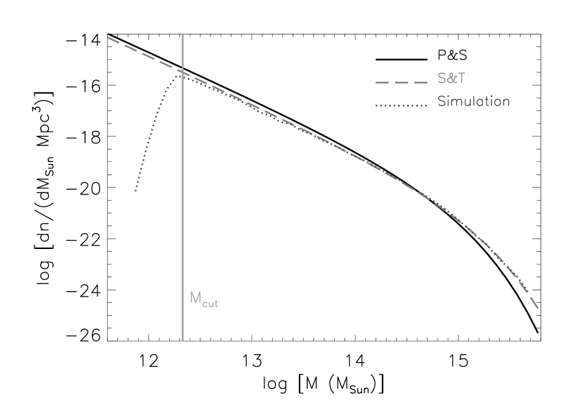
The mass function of the halo catalogs is then compared both with the analytical Press & Schechter (Press & Schechter, 1974) and with the Sheth & Tormen approximation (Sheth & Tormen, 1999). Because of the limited resolution in the simulation, haloes with too few particles have to be excluded from the catalogue. As shown in Fig. 1, small-mass haloes depart from the Press & Schechter and the Sheth & Tormen mass functions. We include in the halo catalogue only haloes above resolution limits, i.e., above $\rm{M}_{cut}=1.5\times 10^{12}h^{-1}\rm{M}_{\odot}$. The final halo catalogue consists of $2.1\times 10^{6}$ haloes, with masses ranging from $1.5\times 10^{12}h^{-1}\rm{M}_{\odot}$ to $3.7\times 10^{15}h^{-1}\rm{M}_{\odot}$.

In order to consider the effect of the shot-noise, we also generated a random catalogue consisting of as many particles as the number of haloes. This is the reference shot-noise catalogue. It should be noted that the uniformly distributed random haloes do not obey exclusion: real haloes can not be spaced closer than a virial radius. This leads to a slight error in modelling the shot noise, which we neglect.

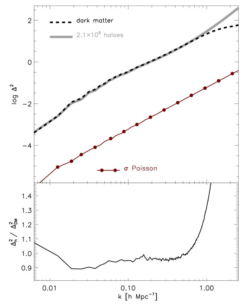
The dimensionless power spectra of the haloes and the dark matter are shown in Fig. 2 together with the Poisson counting error. At small scales ($k\gtrsim 1.0~{}h$ Mpc^-1) the halo power spectrum strongly departs from the dark matter power spectrum. This is because at those scales the halo power spectrum is dominated by the shot noise. As it will be shown in the next section, once we subtract the shot noise, the halo power spectrum will show the same small-scales turn-down as the dark matter power spectrum.

Figure 2: Upper panel: dimensionless power spectrum of the dark matter (black-dotted line) and of the halo catalogue (gray-solid line). The Poisson error is shown with the solid-bullet line. Lower panel: ratio of the halo and the dark matter power spectrum.

4 Stochasticity between haloes of different mass

We start by studying the relation between haloes of different masses. The goal of this section is to use PCA to determine whether different halo populations are coherent or if stochasticity is present and, if present, to determine its behaviour. As we will see below, the eigenvalues of a shot-noise-type field are all the same (‘maximally stochastic scenario’). We want to answer the question: does the stochasticity between haloes of different mass behave in the same manner?

4.1 Applying PCA to the halo covariance matrix

The first step is to divide our simulated haloes into bins, sorted by mass. We present the results obtained by dividing the halo catalogue into 6 bins, but we will show in the next sub-section that the results do not change if we double the number of bins. The bins are chosen with equal number of haloes, such that the shot noise properties between them are similar.

PCA is applied to the covariance matrix $\sigma_{ij}$ between the six halo bins. A brief explanation of the way we apply PCA is given in Appendix A. For each wavemode $k$, the covariance matrix is given by:

$$\sigma_{ij}=\langle\delta_{i}\delta_{j}\rangle$$ (5)

where the indices $i=1,..,n$ and $j=1,..,n$ refer to the halo bins, and where the average is done over wavemodes during the power spectrum and cross-power spectrum calculation.

In the same way as for the haloes, we divide the random catalogue in bins, calculate the power spectrum of each bin and the cross-power spectrum between the bins, and we apply the same procedure of PCA to the covariance matrix from the random catalogue.

Figure 3: Upper panel: Eigenvalues of the halo bins covariance matrix (solid thick lines) and of the random bins covariance matrix (dashed thick Only the first eigenvalue of the halo covariance matrix (darkest solid thick line) is significantly higher than the others, suggesting the absence of stochasticity in the halo correlation. The Poisson error is the same as in the previous figure. Lower panel: Difference between the halo bins eigenvalues and the corresponding eigenvalues from the random catalogue. The first eigenvalue (solid black thick line) is still higher than the others, but we notice here that also the second eigenvalue (long-dashed, dark-gray thick line) tends to be significantly higher than the others at $k\gtrsim 0.05~{}h$ Mpc^-1, suggesting that haloes are minimally stochastic.

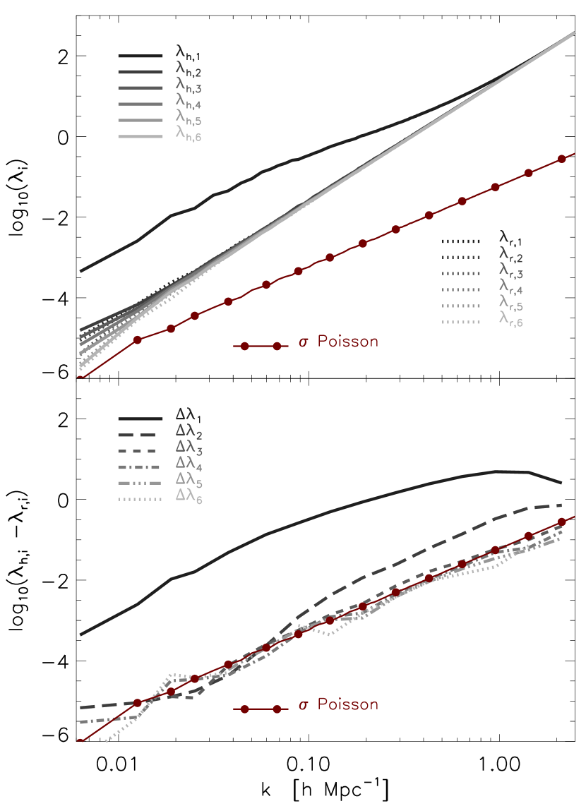
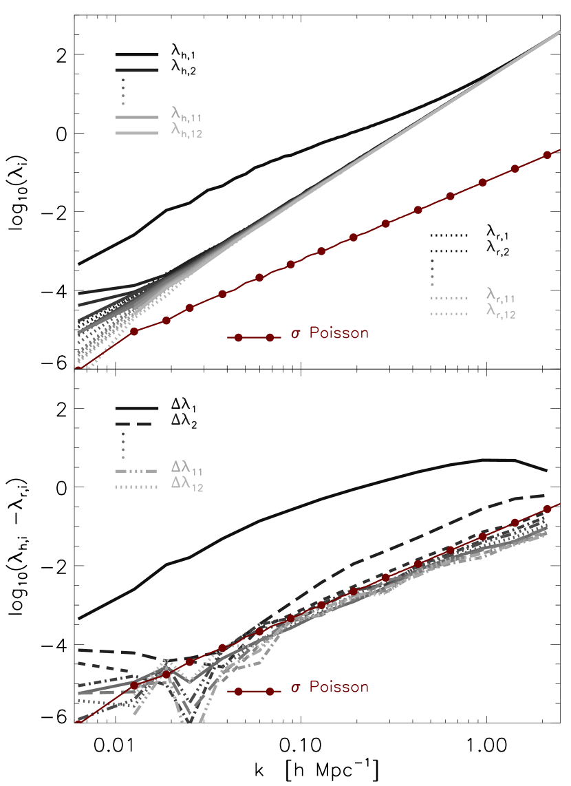
In the upper panel of Fig. 3 we show the eigenvalues of the halo covariance matrix (solid lines) compared to the eigenvalues of the random covariance matrix (dotted lines). The first eigenvalue of the halo catalogue is significantly higher than the others, which in turn are very close to the eigenvalues of the random catalogue. As expected, the shot-noise eigenvalues are all equal to each other (the scatter at small-k is due to counting error).

To test if all the eigenvalues but the first one are a consequence of shot-noise, we subtracted from each halo eigenvalue the corresponding eigenvalue of the random catalogue. The $\Delta\lambda_{i}=\lambda_{i,halo}-\lambda_{i,random}$ are plotted in the lower panel of Fig. 3. In this case, only $\Delta\lambda_{1}$ is the dominant one. But we notice that also $\Delta\lambda_{2}$ is higher than the other differences. This implies that there is one additional, and primarily only one, source of stochasticity other than the Poisson noise. In other words, the detected stochasticity is not a shot-noise like stochasticity. This result is in agreement with what was found by TB99: studying the correlation between four ‘clans’ of galaxies, TB99 found a principal component which traces the matter, which is followed by a second eigenvalue that is significantly larger than the remaining two. Their result was obtained for scales around $k\sim 0.6~{}h~{}\rm{Mpc}^{-1}$, which is within the scales where our second eigenvalue dominates.

It’s clear that this scatter in the relation between different populations is due to a lack of further information on the populations. Using PCA we can not further determine on the origin of this scatter, and this is beyond the goal of the present work. Recent studies have shown that bias between haloes and dark matter (and therefore between different haloes populations) could depend on other physical properties other than halo mass, such as halo formation time (e.g. Gao et al., 2005; Gao & White, 2007) and concentration (Wechsler et al., 2006). In principle, one could test any possible ingredient by applying PCA to a $N^{P}\times N^{P}$ covariance matrix, where $N$ is the number of bins used and $P$ is the number of parameters included.

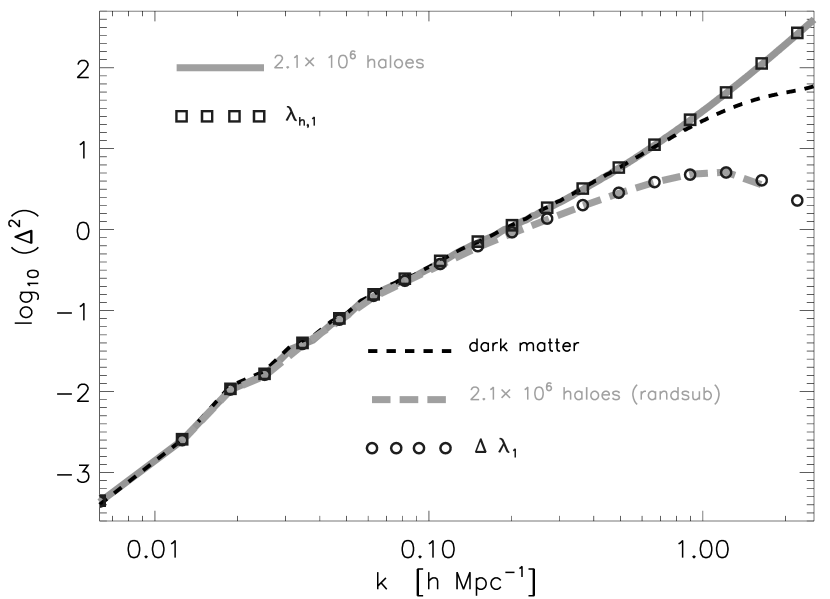
Finally, as a check for the fact that most of the signal is contained in the first eigenvalue, we compare $\lambda_{1}$ with the dimensionless power spectrum of the complete halo catalogue. As shown in Fig. 4 the first eigenvalue follows the halo $\Delta^{2}$, both in the case of shot-noise and non shot-noise subtraction. The random-subtracted halo $\Delta^{2}$ is now lower than the dark matter $\Delta^{2}$ at smaller scales, because we are neglecting here the correlation of structures within haloes (the 1-halo term).

Figure 4: $\Delta^{2}$ of the halo catalogue, both before and after random subtraction (respectively gray solid and gray long-dashed lines). The first eigenvalue is shown by the symbols, again both before and after random subtraction (respectively squares and circles). The random-subtracted halo power spectrum is now lower than the DM power spectrum (thin dashed black line) at small scales, because we are neglecting here the 1-halo term.

4.2 Results with a different number of bins

To test how the results described in the previous sub-section depend on the number of bins used, we repeated the same exercise using $12$ bins. As show in Fig.5 the outcome is the same: we find that there is only one stochastic component other than the shot noise, i.e., haloes are ‘minimally stochastic’. The only difference is a slightly higher scatter in the eigenvalues at small wavemodes, due to the smaller number of objects in each bin.

Figure 5: Same as Fig. 3, but with a higher number of halo bins.

5 Stochasticity between dark matter and halo bins

In this section we first show how eigenvectors can be used to trace the bias. We then study the stochasticity between haloes and dark matter, confirming that stochasticity saturates at scales where the $\Lambda$CDM power spectrum peaks. Finally, we show how stochasticity can be reduced when the halo density field is weighted using the principal component from the previous section.

5.1 Bias and Eigenvectors

Figure 6: Bias between haloes of different mass and dark matter (solid lines), compared to the components of the first eigenvector. The shot-noise has been previously subtracted. The higher biases (darker lines) correspond to bins with higher mass haloes.

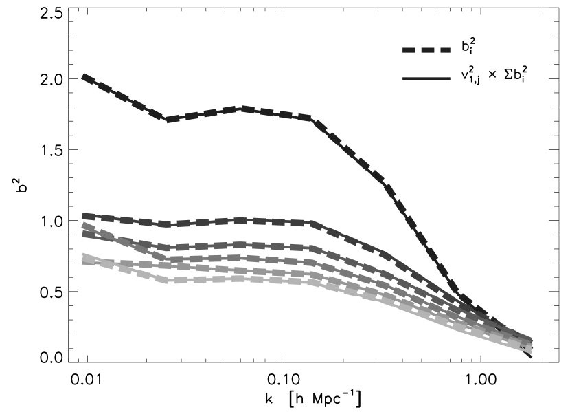
The bias between the haloes, random subtracted, and the dark matter is shown in Fig.6, where the highest value of the bias is the one related to the bin with higher-mass haloes. In the same figure we also plotted the components of the principal component, i.e., the eigenvector corresponding to the first eigenvalue derived in the previous section. When multiplied by the sum of all the bias at each $k$, the square of the components of the first eigenvector follow the bias between the corresponding halo bin and the dark matter. This is straightforward to demonstrate when $r=1$. In this scenario, in fact, the covariance is simply given by:

$$\sigma_{ij}=b_{i}b{j}$$ (6)

In the two-dimensional case, for example, we have:

$$\sigma_{ij}=\left(\begin{array}[]{cc}b_{1}^{2}&b_{1}b_{2}\\ b_{1}b_{2}&b_{2}^{2}\\ \end{array}\right)$$ (7)

and it is straightforward to show that the principal component of this matrix is: $v_{1}=(b_{1},b_{2})$. The bias between different populations can therefore be approximated by the eigenvectors of the covariance matrix, at scales where $r\simeq 1$ (see also TB99).

5.2 Stochasticity

We now explore in details the behaviour of stochasticity between haloes and dark matter.

Figure 7: Cross-correlation coefficients $r$ between the halo bins and the dark matter. In the lower panel $r$ is shot-noise subtracted.

Figure 8: $\mathcal{S}=\sqrt{2(1-r)}$ between halo bins and DM. In the lower panel $\mathcal{S}$ is shot-noise subtracted.

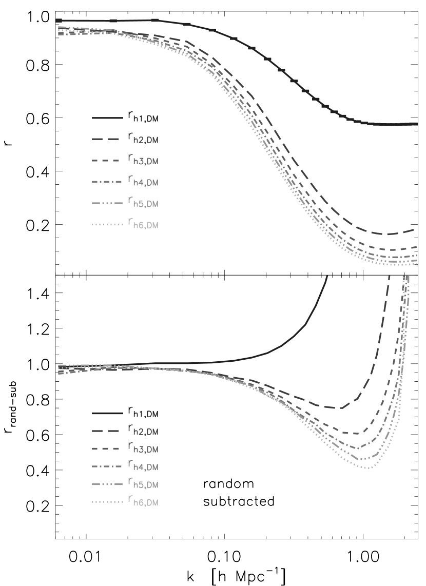
The cross-correlation coefficients between each halo bin and the dark matter is shown in Fig. 7 as a function of the wavemode $k$. In all cases, the coefficient is close to $1$ at large scales (i.e., lower values of $k$), but it approaches $0$ at higher values of k, with a more abrupt decrease in the case of less massive haloes.

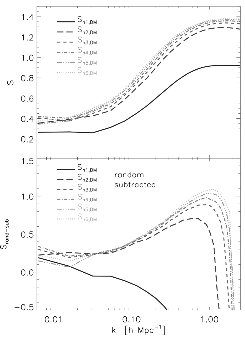
$r$ is indeed close to $1$ at large scales, as it as been always assumed in works involving the relation between dark matter and haloes (or galaxies), but io order to verify how good this assumption is, and to determine the effect of even a small departure of $r$ from unity, we consider the quantity $\mathcal{S}=\sqrt{2(1-r)}$, which is plotted in Fig. 8. Even when $r$ is closest to unity we have $\mathcal{S}\simeq 0.2$, which implies an error of $\simeq 20$ per cent in the relation between the halo and the dark matter density fields. As expected, stochasticity saturates ($\mathcal{S}$ becomes flat) at $k\la 0.02~{}h~{}\rm{Mpc}^{-1}$, which corresponds to the peak of the $\Lambda$CDM power spectrum (e.g., Dodelson et al., 1996). If stochasticity is due to a local process, one expects its power to be flat at large scales. The stochasticity thus decreases with increasing large scale power. At large scales ($k\la 0.02~{}h~{}\rm{Mpc}^{-1}$, the power spectrum drops, and one would expect a minimum in the stochasticity, which we indeed observe.

Figure 9: Cross-correlation coefficient $r$ between the haloes and the dark matter, both in the weighted and in the non-weighted case. In the upper panel the haloes are weighted using the first three eigenvectors, but only the principal component (i.e., the first eigenvector) is significant. In the lower panel the same result is shown after the subtraction of the noise.

Figure 10: Same as previous figure for the quantity $\mathcal{S}=\sqrt{2(1-r)}$.

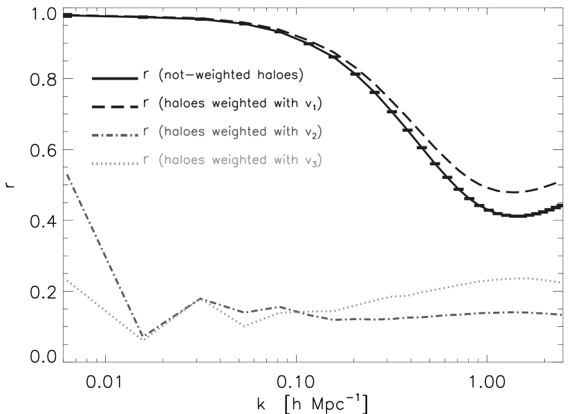
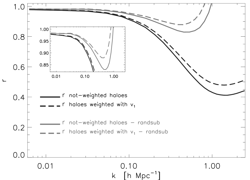
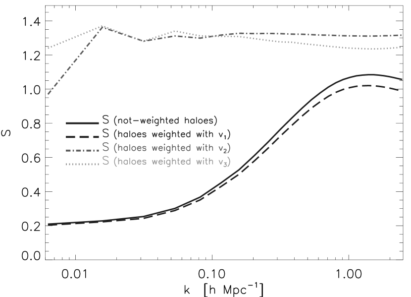
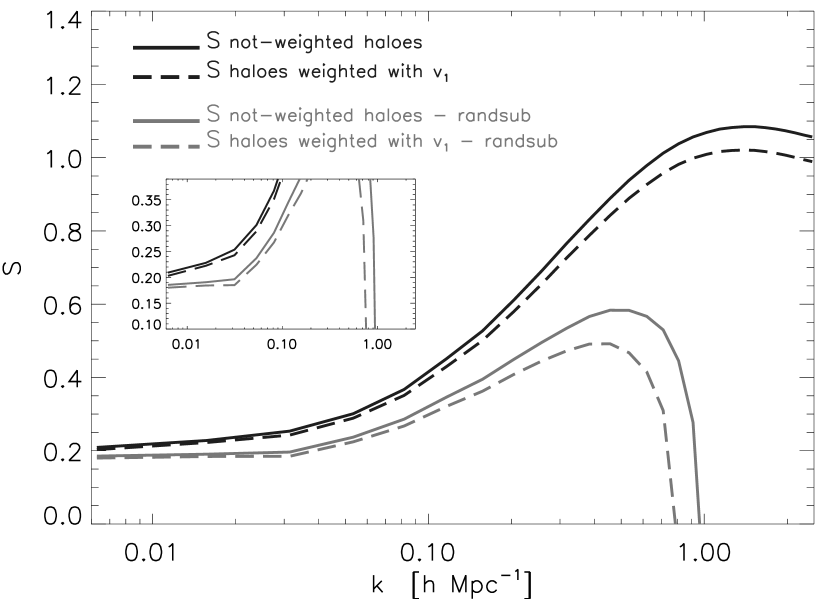
The values of $r$ and $\mathcal{S}$ are shown both before and after the shot-noise subtraction. Notice that, because of the subtraction of the noise, the value of $r$ can become greater than $1$, in which case $\sqrt{2(1-r)}$ can be non-real. We still show $\mathcal{S}$, considering that we calculate $\sqrt{2(1-r)}$ taking $|1-r|$, and assigning at $\mathcal{S}$ the sign of $(1-r)$. Even after the shot-noise subtraction, the scatter in the bias saturates at large scales, and it is of the order of $15$ per cent.

5.3 Using the principal component as weight

Figure 11: Error on the cross-correlation coefficient. For visualization purposes, the error bars have been centered at zero.

Figure 12: Density maps of the haloes. In the first one, the haloes have been weighted using the principal component at $k=0.01885$. The second one is weighted using the second eigenvector and the third maps using the third one.

The results of the previous sub-section are now shown using the ‘weighted’ values of the halo power spectrum: in the calculation of $\Delta^{2}$ for the halo catalogue, the particle masses are multiplied by a weight depending on which mass-bin they belong to. The weights are given by the components of the eigenvectors obtained when diagonalizing the covariance matrix of the $n$ halo bins.

From statistical theory, assuming to have $k$ independent estimates $e_{i}$ of the quantity to be measured, each with the associated error $\sigma_{i}$, the best combined estimate is the weighted mean, given by:

$$\overline{e}=\frac{\sum_{i=1}^{k}w_{i}\overline{e_{i}}}{\sum_{i=1}^{k}w_{i}}$$ (8)

where the weights are given by $w_{i}=1/\sigma_{i}^{2}$.

In our case the dark matter density field is given by equation (1) plus an error $\sigma_{noise}$:

$$\delta_{h,i}^{2}=b_{i}^{2}\delta_{DM}^{2}\pm\sigma_{noise}\\$$ (9)

where again $i$ refers to the halo bin considered. Dividing all quantities by the bias, and using equation (8), we obtain:

$$\overline{\delta_{DM}^{2}}=\frac{\sum_{i}^{n}b_{i}^{2}\delta^{2}_{h,i}}{\sum_{i}^{n}b_{i}^{2}}$$ (10)

We see that in our case the weight for each bin is given by the square of the corresponding bias. Using the eigenvectors has advantages over dividing the power of the bins: when fine bins are used, the shot noise increases. Unless stochasticity dominates, more information is used when using the eigenvector, which includes all cross correlations to measure the bias.

Since the bias is not a measurable quantity in observations, we use as weights for each bin the corresponding components of the principal component. As was shown at the beginning of this section, $b^{2}_{i}\equiv v^{2}_{1,j}\times\sum_{i=1}^{n}b^{2}_{i}$ when $r=1$. Therefore we effectively use as weights the components of the first eigenvector corresponding to the wavemode $k=0.01885~{}h~{}\rm{Mpc}^{-1}$, the wavemode at which the cross-correlation coefficient is closest to $1$. At each $k$ there are $6$ eigenvectors, since $r$ is not perfectly equal to $1$, and each of them has $6$ components. We first weighted the bins using the components of the principal component: the mass of the particles belonging to the bin $j$ have been multiplied by the $j$th component of $v_{1,j}$. We repeated this exercise also using the components of second and third eigenvector.

In Fig. 9, the cross-correlation coefficient between the entire halo catalogue and the dark matter is shown both in the weighted and non-weighted case. When weighted using the first eigenvector, the value of $r$ gets closer to $1$ at every $k$, and the increase is more substantial at larger wavemode. We see how the weighting done using the eigenvectors corresponding to the secondary components corresponds to low values of the cross-correlation coefficient, and this is because these components correspond to noise.

Again, to see how the weighting process changes stochasticity, we calculate the quantity $\sqrt{2(1-r)}$, which is shown in Fig. 10 as a function of $k$. In this case, the minimum error in the relation between the entire halo population and the dark matter density field is $\sim 18$ per cent.

We need to check if the statistical measurement error in the data coming from the simulation could be the cause of the departure of $r$ from unity. We show that this can not be the case, and the error on $r$ is small. As derived in appendix B, $\Delta r$ as a function of scale is given by: $\Delta r(k)=\langle\epsilon^{2}(\mathbf{k})\rangle/\langle\delta^{2}_{DM}(\mathbf{k})\rangle$, where $\epsilon^{2}$ is the random density field. $\Delta r$ is shown in Fig. 11, where the error bars have been centered at $0$. The small values of $\Delta r$ make it insignificant with respect to $r$, and even when considering possible effects of the error, $r$ can not reach the unity.

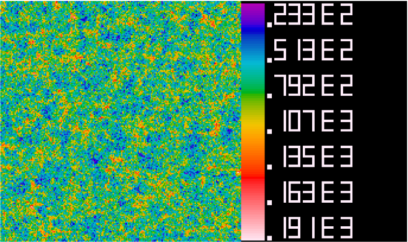
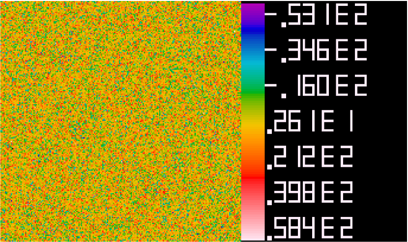
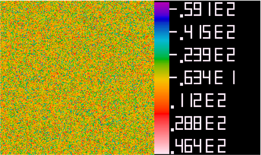
The density maps of the haloes, properly weighted using the first 3 eigenvectors corresponding to $k=0.01885~{}h~{}\rm{Mpc}^{-1}$ are shown in Fig. 12.

As for the previous section, these last results do not depend on the number of bins used. To avoid redundancy, we omit the plots.

6 Summary and Conclusions

We studied the correlation between different halo populations and between haloes and dark matter using a PCA technique. To do so, we used the output of a N-body simulation with $1624^{3}$ particles in a $1000h^{-1}\rm{Mpc}$ box. After dividing the halo catalogue into bins sorted by mass, we applied PCA to the covariance matrix given by the cross-power spectra of the halo bins.

Analyzing the haloes alone, we now understand the stochasticity between haloes of different mass: we have one dominant principal component, and a second component which is small and grows in relative importance as one approaches the non-linear scales. This component dominates the apparent stochasticity. The remaining components are all at the level expected from random sampling. We call this ‘minimal stochasticity’, which is the opposite scenario from what one might expect in a shot noise model, which we called ‘maximally stochastic’. This result is in agreement with the conclusions of Tegmark & Bromley (1999), who studied the correlation between different galaxy populations.

When we consider the relation between haloes and dark matter, we find that the highest eigenvalue is the best tracer of dark matter. Even though this is the best that can be done, the error is still at least of the order of $15$ per cent, even at very large scales, and at $\lambda\ga 300h^{-1}\rm{Mpc}$ stochasticity is saturated as expected: at this scale the dark matter power spectrum reaches its peak (for a $\Lambda$CDM cosmology). Moreover, we show that the eigenvectors from PCA are a better estimate for the bias, since it takes into account all pairs of bins, and has less shot noise.

We also studied the correlation of halo mass bins, and the PCA eigenvectors, with the total underlying dark matter. The observation of galaxies and the measure of their power spectra can provide useful information on the distribution of dark matter if bias and stochasticity are properly considered. When we use the components of the principal component as weights for the calculation of the power spectra of the haloes, the estimate of the dark matter power spectra improves further.

We argue that this is a better way to properly calculate the galaxy power spectra and then estimate the underlying dark matter power spectra and to properly estimate the bias between galaxies of different luminosity and dark matter.

Appendix A PCA

Principal Component Analysis is used to identify patterns in data, and to highlight how data are related to each other. The first step is to calculate the covariance matrix of the data set. The dimension of the matrix $n$ is equal to the dimension of the data set. The covariance matrix is defined as:

$$\sigma_{ij}\equiv\langle(x_{i}-\mu_{i})(x_{j}-\mu_{j})\rangle$$ (11)

where $i=1,..,n$, $j=1,..,n$ and $\mu$ indicates the mean of the data for the considered dimension. The main diagonal, $i=j$, is given by the variances of the data in that dimension, and the matrix is symmetric.

PCA calculates the eigenvectors and the corresponding eigenvalues of a covariance matrix. The eigenvector associated with the highest eigenvalue is the principal component of the data set, and it indicates the main direction along which the data are distributed. The smaller an eigenvalue, the smaller the ‘significance’ of that component.

In summary, the number of significant eigenvalues indicates on how many directions the data are spread. A data set is considered stochastic if more than one eigenvalue are different from zero, and deterministic if only one eigenvalue is not null, in which case, if you know one data point you know them all. In this paper we generalize the nature of stochasticity to depend on the nature of the eigenvalues. If all modes have an equal eigenvalue, as in shot noise, we call it ‘maximal stochasticity’, while a single mode which dominates the stochasticity is called ‘minimal stochasticity’.

Appendix B Errors

B.1 Spread of the error when binning

Throughtout the paper, we often bin along the wavemode $k$. Quantities which depend on $k$ will then be averaged out within the $k-$bins. If $\sigma_{k,x}$ are the rms fluctuations of the quantity $x(k)$, from basics of statistics the new error $\sigma_{k_{new},x}$ on each new average $x(k_{new})$, is given by:

$$\sigma_{k_{new},x}=\left(\frac{\sum_{k_{min}}^{k_{max}}\sigma^{2}_{k,x}}{N^{2}_{k,bin}}\right)^{1/2}$$ (12)

where $k_{min}$ and $k_{max}$ are the extremes of the bin centered in $k_{new}$, and $N^{2}_{k,bin}$ is the number of wavemodes contained in each bin.

B.2 Errors on $r$ and $\mathcal{S}$

We derive the error on $r$ assuming $r=1$ (No stochasticity null-hypothesis). The cross-correlation coefficient between haloes and dark matter is given by:

$$r(k)=\frac{\langle\delta_{h}(\mathbf{k})\delta_{DM}(\mathbf{k})\rangle}{\sqrt{\langle\delta^{2}_{h}(\mathbf{k})\rangle\langle\delta^{2}_{DM}(\mathbf{k})\rangle}}$$ (13)

If there is no stochasticity, we have $\langle\delta^{2}_{h}\rangle=\langle\delta^{2}_{DM}\rangle+\langle\epsilon^{2}\rangle$, where $\epsilon^{2}$ is the random density field. The cross-correlation coefficient then becomes:

$$r(k)=\frac{\langle(\delta_{DM}(\mathbf{k})+\epsilon(\mathbf{k}))\delta_{DM}(\mathbf{k})\rangle}{\sqrt{\langle\delta^{2}_{DM}(\mathbf{k})\rangle(\langle\delta^{2}_{h}(\mathbf{k})\rangle-\langle\epsilon^{2}(\mathbf{k})\rangle)}}$$ (14)

where, in the denominator, we subtract the random field from the halo bin.

After some simple arithmetic we get to the final steps which show that, in the absence of stochasticity, the cross-correlation coefficient is indeed unity:

$$r(k)=\frac{\langle\delta^{2}_{DM}(\mathbf{k})\rangle+\langle\epsilon(\mathbf{k})\delta_{DM}(\mathbf{k})\rangle}{\langle\delta^{2}_{DM}(\mathbf{k})\rangle}=\frac{\langle\delta^{2}_{DM}(\mathbf{k})\rangle}{\langle\delta^{2}_{DM}(\mathbf{k})\rangle}=1$$ (15)

Note that $\langle\epsilon(\mathbf{k})\delta_{DM}(\mathbf{k})\rangle=0$, where here the average is done over various directions of $\mathbf{k}$ within a simulation.

Now, being $1$ the expectation value of $r$, the error on $r$ is given by:

$$(\Delta r(k))^{2} \equiv \langle(r(k)-1)^{2}\rangle$$ (16)

$$= \langle r^{2}(k)\rangle-1$$

$$= \frac{\langle\delta^{2}_{DM}(\mathbf{k})(\delta_{DM}(\mathbf{k})+\epsilon(\mathbf{k}))^{2}\rangle}{\langle\delta^{2}_{DM}(\mathbf{k})\rangle^{2}}-1$$

$$= \frac{\langle\epsilon^{2}(\mathbf{k})\rangle}{\langle\delta^{2}_{DM}(\mathbf{k})\rangle}$$

where the average is done over an ensamble of simulations.

References

- Cole & Lacey (1996) Cole S., Lacey C., 1996, MNRAS, 281, 716
- Dekel & Lahav (1999) Dekel A., Lahav O., 1999, ApJ, 520, 24
- Dodelson et al. (1996) Dodelson S., Gates E. I., Turner M. S., 1996, Science, 274, 69
- Gao et al. (2005) Gao L., Springel V., White S. D. M., 2005, MNRAS, 363, L66
- Gao & White (2007) Gao L., White S. D. M., 2007, MNRAS, 377, L5
- Guzik & Seljak (2002) Guzik J., Seljak U., 2002, MNRAS, 335, 311
- Hoekstra et al. (2005) Hoekstra H., Hsieh B. C., Yee H. K. C., Lin H., Gladders M. D., 2005, ApJ, 635, 73
- Mandelbaum et al. (2006) Mandelbaum R., et al., 2006, MNRAS, 368, 715
- Meneux et al. (2006) Meneux B., et al., 2006, A&A, 452, 387
- Merz et al. (2005) Merz H., Pen U.-L., Trac H., 2005, New Astronomy, 10, 393
- Mo & White (1996) Mo H. J., White S. D. M., 1996, MNRAS, 282, 347
- Norberg et al. (2002) Norberg P., et al., 2002, MNRAS, 332, 827
- Peacock et al. (2001) Peacock J. A., et al., 2001, Nat, 410, 169
- Pen (1998) Pen U.-L., 1998, ApJ, 504, 601
- Pen (2004) Pen U.-L., 2004, MNRAS, 350, 1445
- Press & Schechter (1974) Press W. H., Schechter P., 1974, ApJ, 187, 425
- Scranton et al. (2005) Scranton R., et al., 2005, ApJ, 633, 589
- Seljak & Warren (2004) Seljak U., Warren M. S., 2004, MNRAS, 355, 129
- Sheth et al. (2001) Sheth R. K., Mo H. J., Tormen G., 2001, MNRAS, 323, 1
- Sheth & Tormen (1999) Sheth R. K., Tormen G., 1999, MNRAS, 308, 119
- Spergel et al. (2003) Spergel D. N., et al., 2003, ApJS, 148, 175
- Swanson et al. (2008) Swanson M. E. C., Tegmark M., Blanton M., Zehavi I., 2008, MNRAS, 385, 1635
- Tegmark & Bromley (1999) Tegmark M., Bromley B. C., 1999, ApJ, 518, L69
- Tegmark et al. (2004a) Tegmark M., et al., 2004a, PhRvD, 69, 103501
- Tegmark et al. (2004b) Tegmark M., et al., 2004b, ApJ, 606, 702
- van den Bosch et al. (2007) van den Bosch F. C., et al., 2007, MNRAS, 376, 841
- Wang et al. (2007) Wang Y., et al., 2007, ArXiv e-prints, 711
- Wechsler et al. (2006) Wechsler R. H., et al., 2006, ApJ, 652, 71
- Wild et al. (2005) Wild V., et al., 2005, MNRAS, 356, 247
- Zehavi et al. (2005) Zehavi I., et al., 2005, ApJ, 621, 22
- Zhang & Pen (2005) Zhang P., Pen U.-L., 2005, Physical Review Letters, 95, 241302
- Zhang & Pen (2006) Zhang P., Pen U.-L., 2006, MNRAS, 367, 169