MultiNest: an efficient and robust Bayesian inference tool for cosmology and particle physics

Abstract

We present further development and the first public release of our multimodal nested sampling algorithm, called MultiNest. This Bayesian inference tool calculates the evidence, with an associated error estimate, and produces posterior samples from distributions that may contain multiple modes and pronounced (curving) degeneracies in high dimensions. The developments presented here lead to further substantial improvements in sampling efficiency and robustness, as compared to the original algorithm presented in Feroz & Hobson (2008), which itself significantly outperformed existing MCMC techniques in a wide range of astrophysical inference problems. The accuracy and economy of the MultiNest algorithm is demonstrated by application to two toy problems and to a cosmological inference problem focussing on the extension of the vanilla $\Lambda$CDM model to include spatial curvature and a varying equation of state for dark energy. The MultiNest software, which is fully parallelized using MPI and includes an interface to CosmoMC, is available at http://www.mrao.cam.ac.uk/software/multinest/. It will also be released as part of the SuperBayeS package, for the analysis of supersymmetric theories of particle physics, at http://www.superbayes.org

1 Introduction

Bayesian analysis methods are already widely used in astrophysics and cosmology, and are now beginning to gain acceptance in particle physics phenomenology. As a consequence, considerable effort has been made to develop efficient and robust methods for performing such analyses. Bayesian inference is usually considered to divide into two categories: parameter estimation and model selection. Parameter estimation is typically performed using Markov chain Monte Carlo (MCMC) sampling, most often based on the standard Metropolis–Hastings algorithm or its variants, such as Gibbs’ or Hamiltonian sampling (see e.g. Mackay 2003). Such methods can be very computationally intensive, however, and often experience problems in sampling efficiently from a multimodal posterior distribution or one with large (curving) degeneracies between parameters, particularly in high dimensions. Moreover, MCMC methods often require careful tuning of the proposal distribution to sample efficiently, and testing for convergence can be problematic. Bayesian model selection has been further hindered by the even greater computational expense involved in the calculation to sufficient precision of the key ingredient, the Bayesian evidence (also called the marginalized likelihood or the marginal density of the data). As the average likelihood of a model over its prior probability space, the evidence can be used to assign relative probabilities to different models (for a review of cosmological applications, see Mukherjee et al. 2006). The existing preferred evidence evaluation method, again based on MCMC techniques, is thermodynamic integration (see e.g. Ó Ruanaidh & Fitzgerald 1996), which is extremely computationally intensive but has been used successfully in astronomical applications (see e.g. Hobson & McLachlan 2003; Marshall et al. 2003; Slosar A. et al. 2003; Niarchou et al. 2004; Bassett et al. 2004; Trotta 2007; Beltrán et al. 2005; Bridges et al. 2006). Some fast approximate methods have been used for evidence evaluation, such as treating the posterior as a multivariate Gaussian centred at its peak (see e.g. Hobson et al. 2002), but this approximation is clearly a poor one for multimodal posteriors (except perhaps if one performs a separate Gaussian approximation at each mode). The Savage–Dickey density ratio has also been proposed (Trotta 2005) as an exact, and potentially faster, means of evaluating evidences, but is restricted to the special case of nested hypotheses and a separable prior on the model parameters. Various alternative information criteria for astrophysical model selection are discussed by Liddle (2007), but the evidence remains the preferred method.

Nested sampling (Skilling 2004) is a Monte Carlo method targetted at the efficient calculation of the evidence, but also produces posterior inferences as a by-product. In cosmological applications, Mukherjee et al. (2006) showed that their implementation of the method requires a factor of $\sim 100$ fewer posterior evaluations than thermodynamic integration. To achieve an improved acceptance ratio and efficiency, their algorithm uses an elliptical bound containing the current point set at each stage of the process to restrict the region around the posterior peak from which new samples are drawn. Shaw et al. (2007) point out that this method becomes highly inefficient for multimodal posteriors, and hence introduce the notion of clustered nested sampling, in which multiple peaks in the posterior are detected and isolated, and separate ellipsoidal bounds are constructed around each mode. This approach significantly increases the sampling efficiency. The overall computational load is reduced still further by the use of an improved error calculation (Skilling 2004) on the final evidence result that produces a mean and standard error in one sampling, eliminating the need for multiple runs. In our previous paper (Feroz & Hobson 2008 – hereinafter FH08), we built on the work of Shaw et al. (2007) by pursuing further the notion of detecting and characterising multiple modes in the posterior from the distribution of nested samples, and presented a number of innovations that resulted in a substantial improvement in sampling efficiency and robustness, leading to an algorithm that constituted a viable, general replacement for traditional MCMC sampling techniques in astronomical data analysis.

In this paper, we present further substantial development of the method discussed in FH08 and make the first public release of the resulting Bayesian inference tool, called MultiNest. In particular, we propose fundamental changes to the ‘simultaneous ellipsoidal sampling’ method described in FH08, which result in a substantially improved and fully parallelized algorithm for calculating the evidence and obtaining posterior samples from distributions with (an unkown number of) multiple modes and/or pronounced (curving) degeneracies between parameters. The algorithm also naturally identifies individual modes of a distribution, allowing for the evaluation of the ‘local’ evidence and parameter constraints associated with each mode separately.

The outline of the paper is as follows. In Section 2, we briefly review the basic aspects of Bayesian inference for parameter estimation and model selection. In Section 3, we introduce nested sampling and discuss the use of ellipsoidal bounds in Section 4. In Section 5, we present the MultiNest algorithm. In Section 6, we apply our new algorithms to two toy problems to demonstrate the accuracy and efficiency of the evidence calculation and parameter estimation as compared with other techniques. In Section 7, we consider the use of our new algorithm for cosmological model selection focussed on the extension of the vanilla $\Lambda$CDM model to include spatial curvature and a varying equation of state for dark energy. We compare the efficiency of MultiNest and standard MCMC techniques for cosmological parameter estimation in Section 7.3. Finally, our conclusions are presented in Section 8.

2 Bayesian Inference

Bayesian inference methods provide a consistent approach to the estimation of a set parameters $\mathbf{\Theta}$ in a model (or hypothesis) $H$ for the data $\mathbf{D}$. Bayes’ theorem states that

$$\Pr(\mathbf{\Theta}|\mathbf{D},H)=\frac{\Pr(\mathbf{D}|\,\mathbf{\Theta},H)\Pr(\mathbf{\Theta}|H)}{\Pr(\mathbf{D}|H)},$$ (1)

where $\Pr(\mathbf{\Theta}|\mathbf{D},H)\equiv\mathcal{P}(\mathbf{\Theta})$ is the posterior probability distribution of the parameters, $\Pr(\mathbf{D}|\mathbf{\Theta},H)\equiv\mathcal{L}(\mathbf{\Theta})$ is the likelihood, $\Pr(\mathbf{\Theta}|H)\equiv\pi(\mathbf{\Theta})$ is the prior, and $\Pr(\mathbf{D}|H)\equiv\mathcal{Z}$ is the Bayesian evidence.

In parameter estimation, the normalising evidence factor is usually ignored, since it is independent of the parameters $\mathbf{\Theta}$, and inferences are obtained by taking samples from the (unnormalised) posterior using standard MCMC sampling methods, where at equilibrium the chain contains a set of samples from the parameter space distributed according to the posterior. This posterior constitutes the complete Bayesian inference of the parameter values, and can be marginalised over each parameter to obtain individual parameter constraints.

In contrast to parameter estimation problems, in model selection the evidence takes the central role and is simply the factor required to normalize the posterior over $\mathbf{\Theta}$:

$$\mathcal{Z}=\int{\mathcal{L}(\mathbf{\Theta})\pi(\mathbf{\Theta})}d^{D}\mathbf{\Theta},$$ (2)

where $D$ is the dimensionality of the parameter space. As the average of the likelihood over the prior, the evidence automatically implements Occam’s razor: a simpler theory with compact parameter space will have a larger evidence than a more complicated one, unless the latter is significantly better at explaining the data. The question of model selection between two models $H_{0}$ and $H_{1}$ can then be decided by comparing their respective posterior probabilities given the observed data set $\mathbf{D}$, as follows

$$\frac{\Pr(H_{1}|\mathbf{D})}{\Pr(H_{0}|\mathbf{D})}=\frac{\Pr(\mathbf{D}|H_{1})\Pr(H_{1})}{\Pr(\mathbf{D}|H_{0})\Pr(H_{0})}=\frac{\mathcal{Z}_{1}}{\mathcal{Z}_{0}}\frac{\Pr(H_{1})}{\Pr(H_{0})},$$ (3)

where $\Pr(H_{1})/\Pr(H_{0})$ is the a priori probability ratio for the two models, which can often be set to unity but occasionally requires further consideration.

Evaluation of the multidimensional integral (2) is a challenging numerical task. The standard technique of thermodynamic integration draws MCMC samples not from the posterior directly but from $\mathcal{L}^{\lambda}\pi$ where $\lambda$ is an inverse temperature that is slowly raised from $\approx 0$ to $1$ according to some annealing schedule. It is possible to obtain accuracies of within 0.5 units in log-evidence via this method, but in cosmological model selection applications it typically requires of order $10^{6}$ samples per chain (with around 10 chains required to determine a sampling error). This makes evidence evaluation at least an order of magnitude more costly than parameter estimation.

3 Nested sampling

Nested sampling (Skilling 2004) is a Monte Carlo technique aimed at efficient evaluation of the Bayesian evidence, but also produces posterior inferences as a by-product. A full discussion of the method is given in FH08, so we give only a briefly description here, following the notation of FH08.

Nested sampling exploits the relation between the likelihood and prior volume to transform the multidimensional evidence integral (Eq. 2) into a one-dimensional integral. The ‘prior volume’ $X$ is defined by $dX=\pi(\mathbf{\Theta})d^{D}\mathbf{\Theta}$, so that

$$X(\lambda)=\int_{\mathcal{L}\left(\mathbf{\Theta}\right)>\lambda}\pi(\mathbf{\Theta})d^{D}\mathbf{\Theta},$$ (4)

where the integral extends over the region(s) of parameter space contained within the iso-likelihood contour $\mathcal{L}(\mathbf{\Theta})=\lambda$. The evidence integral (Eq. 2) can then be written as

$$\mathcal{Z}=\int_{0}^{1}{\mathcal{L}(X)}dX,$$ (5)

where $\mathcal{L}(X)$, the inverse of Eq. 4, is a monotonically decreasing function of $X$. Thus, if one can evaluate the likelihoods $\mathcal{L}_{i}=\mathcal{L}(X_{i})$, where $X_{i}$ is a sequence of decreasing values,

$$0<X_{M}<\cdots<X_{2}<X_{1}<X_{0}=1,$$ (6)

as shown schematically in Fig. 1, the evidence can be approximated numerically using standard quadrature methods as a weighted sum

$$\mathcal{Z}={\textstyle{\displaystyle\sum_{i=1}^{M}}\mathcal{L}_{i}w_{i}}.$$ (7)

In the following we will use the simple trapezium rule, for which the weights are given by $w_{i}=\frac{1}{2}(X_{i-1}-X_{i+1})$. An example of a posterior in two dimensions and its associated function $\mathcal{L}(X)$ is shown in Fig. 1.

Figure 1: Cartoon illustrating (a) the posterior of a two dimensional problem; and (b) the transformed $\mathcal{L}(X)$ function where the prior volumes $X_{i}$ are associated with each likelihood $\mathcal{L}_{i}$.

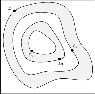
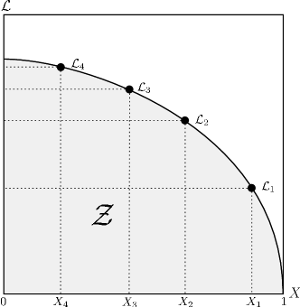
The summation (Eq. 7) is performed as follows. The iteration counter is first set to $i=0$ and $N$ ‘active’ (or ‘live’) samples are drawn from the full prior $\pi(\mathbf{\Theta})$ (which is often simply the uniform distribution over the prior range), so the initial prior volume is $X_{0}=1$. The samples are then sorted in order of their likelihood and the smallest (with likelihood $\mathcal{L}_{0}$) is removed from the active set (hence becoming ‘inactive’) and replaced by a point drawn from the prior subject to the constraint that the point has a likelihood $\mathcal{L}>\mathcal{L}_{0}$. The corresponding prior volume contained within this iso-likelihood contour will be a random variable given by $X_{1}=t_{1}X_{0}$, where $t_{1}$ follows the distribution $\Pr(t)=Nt^{N-1}$ (i.e. the probability distribution for the largest of $N$ samples drawn uniformly from the interval $[0,1]$). At each subsequent iteration $i$, the removal of the lowest likelihood point $\mathcal{L}_{i}$ in the active set, the drawing of a replacement with $\mathcal{L}>\mathcal{L}_{i}$ and the reduction of the corresponding prior volume $X_{i}=t_{i}X_{i-1}$ are repeated, until the entire prior volume has been traversed. The algorithm thus travels through nested shells of likelihood as the prior volume is reduced. The mean and standard deviation of $\log t$, which dominates the geometrical exploration, are $E[\log t]=-1/N$ and $\sigma[\log t]=1/N$. Since each value of $\log t$ is independent, after $i$ iterations the prior volume will shrink down such that $\log X_{i}\approx-(i\pm\sqrt{i})/N$. Thus, one takes $X_{i}=\exp(-i/N)$.

The algorithm is terminated on determining the evidence to some specified precision (we use 0.5 in log-evidence): at iteration $i$, the largest evidence contribution that can be made by the remaining portion of the posterior is $\Delta{\mathcal{Z}}_{i}=\mathcal{L}_{\rm max}X_{i}$, where $\mathcal{L}_{\rm max}$ is the maximum likelihood in the current set of active points. The evidence estimate (Eq. 7) may then be refined by adding a final increment from the set of $N$ active points, which is given by

$$\Delta Z=\sum_{j=1}^{N}\mathcal{L}_{j}w_{M+j},$$ (8)

where $w_{M+j}=X_{M}/N$ for all $j$. The final uncertainty on the calculated evidence may be straightforwardly estimated from a single run of the nested sampling algorithm by calculating the relative entropy of the full sequence of samples (see FH08).

Once the evidence $\mathcal{Z}$ is found, posterior inferences can be easily generated using the full sequence of (inactive and active) points generated in the nested sampling process. Each such point is simply assigned the weight

$$p_{j}=\frac{\mathcal{L}_{j}w_{j}}{\mathcal{Z}}.,$$ (9)

where the sample index $j$ runs from 1 to $\mathcal{N}=M+N$, the total number of sampled points. These samples can then be used to calculate inferences of posterior parameters such as means, standard deviations, covariances and so on, or to construct marginalised posterior distributions.

4 Ellipsoidal nested sampling

The most challenging task in implementing the nested sampling algorithm is drawing samples from the prior within the hard constraint $\mathcal{L}>\mathcal{L}_{i}$ at each iteration $i$. Employing a naive approach that draws blindly from the prior would result in a steady decrease in the acceptance rate of new samples with decreasing prior volume (and increasing likelihood).

Ellipsoidal nested sampling (Mukherjee et al., 2006) tries to overcome the above problem by approximating the iso-likelihood contour $\mathcal{L}=\mathcal{L}_{i}$ by a $D$-dimensional ellipsoid determined from the covariance matrix of the current set of active points. New points are then selected from the prior within this ellipsoidal bound (usually enlarged slightly by some user-defined factor) until one is obtained that has a likelihood exceeding that of the removed lowest-likelihood point. In the limit that the ellipsoid coincides with the true iso-likelihood contour, the acceptance rate tends to unity.

Figure 2: Cartoon of ellipsoidal nested sampling from a simple bimodal distribution. In (a) we see that the ellipsoid represents a good bound to the active region. In (b)-(d), as we nest inward we can see that the acceptance rate will rapidly decrease as the bound steadily worsens. Figure (e) illustrates the increase in efficiency obtained by sampling from each clustered region separately.

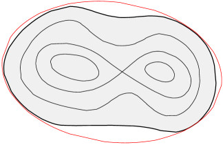
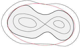
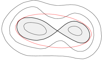
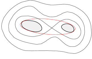
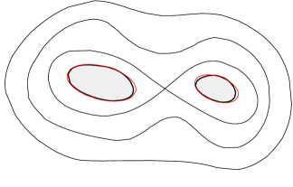
Ellipsoidal nested sampling as described above is efficient for simple unimodal posterior distributions without pronounced degeneracies, but is not well suited to multimodal distributions. As advocated by Shaw et al. (2007) and shown in Fig. 2, the sampling efficiency can be substantially improved by identifying distinct clusters of active points that are well separated and constructing an individual (enlarged) ellipsoid bound for each cluster. In some problems, however, some modes of the posterior may exhibit a pronounced curving degeneracy so that it more closely resembles a (multi–dimensional) ‘banana’. Such features are problematic for all sampling methods, including that of Shaw et al. (2007).

In FH08, we made several improvements to the sampling method of Shaw et al. (2007), which significantly improved its efficiency and robustness. Among these, we proposed a solution to the above problem by partitioning the set of active points into as many sub–clusters as possible to allow maximum flexibility in following the degeneracy. These clusters are then enclosed in ellipsoids and a new point is then drawn from the set of these ‘overlapping’ ellipsoids, correctly taking into account the overlaps. Although this sub-clustering approach provides maximum efficiency for highly degenerate distributions, it can result in lower efficiencies for relatively simpler problems owing to the overlap between the ellipsoids. Also, the factor by which each ellipsoid was enlarged was chosen arbitrarily. Another problem with the our previous approach was in separating modes with elongated curving degeneracies. We now propose solutions to all these problems, along with some additional modifications to improve efficiency and robustness still further, in the MultiNest algorithm presented in the following section.

5 The MultiNest algorithm

The MultiNest algorithm builds upon the ‘simultaneous ellipsoidal nested sampling method’ presented in FH08, but incorporates a number of improvements. In short, at each iteration $i$ of the nested sampling process, the full set of $N$ active points is partitioned and ellipsoidal bounds constructed using a new algorithm presented in Section 5.2 below. This new algorithm is far more efficient and robust than the method used in FH08 and automatically accommodates elongated curving degeneracies, while maintaining high efficiency for simpler problems. This results in a set of (possibly overlapping) ellipsoids. The lowest-likelihood point from the full set of $N$ active points is then removed (hence becoming ‘inactive’) and replaced by a new point drawn from the set of ellipsoids, correctly taking into account any overlaps. Once a point becomes inactive it plays no further part in the nested sampling process, but its details remain stored. We now discuss the MultiNest algorithm in detail.

5.1 Unit hypercube sampling space

The new algorithm for partitioning the active points into clusters and constructing ellipsoidal bounds requires the points to be uniformly distributed in the parameter space. To satisfy this requirement, the MultiNest ‘native’ space is taken as a $D$-dimensional unit hypercube (each parameter value varies from 0 to 1) in which samples are drawn uniformly. All partitioning of points into clusters, construction of ellipsoidal bounds and sampling are performed in the unit hypercube.

In order to conserve probability mass, the point $\textbf{{u}}=(u_{1},u_{2},\cdots,u_{D})$ in the unit hypercube should be transformed to the point $\mathbf{\Theta}=(\theta_{1},\theta_{2},\cdots,\theta_{D})$ in the ‘physical’ parameter space, such that

$$\int\pi(\theta_{1},\theta_{2},\cdots,\theta_{D})\,d\theta_{1}\,d\theta_{2}\cdots d\theta_{D}=\int du_{1}du_{2}\cdots du_{D}.$$ (10)

In the simple case that the prior $\pi(\mathbf{\Theta})$ is separable

$$\pi(\theta_{1},\theta_{2},\cdots,\theta_{D})=\pi_{1}(\theta_{1})\pi_{2}(\theta_{2})\cdots\pi_{D}(\theta_{D}),$$ (11)

one can satisfy Eq. 10 by setting

$$\pi_{j}(\theta_{j})d\theta_{j}=du_{j}.$$ (12)

Therefore, for a given value of $u_{j}$, the corresponding value of $\theta_{j}$ can be found by solving

$$u_{j}=\int_{-\infty}^{\theta_{j}}\pi_{j}(\theta^{\prime}_{j})d\theta^{\prime}_{j}.$$ (13)

In the more general case in which the prior $\pi(\mathbf{\Theta})$ is not separable, one instead writes

$$\pi(\theta_{1},\theta_{2},\cdots,\theta_{D})=\pi_{1}(\theta_{1})\pi_{2}(\theta_{2}|\theta_{1})\cdots\pi_{D}(\theta_{D}|\theta_{1},\theta_{2}\cdots\theta_{D-1})$$ (14)

where we define

$$\pi_{j}(\theta_{j}|\theta_{1},\cdots,\theta_{j-1})$$ (15)

$$=\int\pi(\theta_{1},\cdots,\theta_{j-1},\theta_{j},\theta_{j+1},\cdots,\theta_{D})\,d\theta_{j+1}\cdots d\theta_{D}.$$

The physical parameters $\mathbf{\Theta}$ corresponding to the parameters u in the unit hypercube can then be found by replacing the distributions $\pi_{j}$ in Eq. 13 with those defined in Eq. 15 and solving for $\theta_{j}$. The corresponding physical parameters $\mathbf{\Theta}$ are then used to calculate the likelihood value of the point u in the unit hypercube.

It is worth mentioning that in many problems the prior $\pi(\mathbf{\Theta})$ is uniform, in which case the unit hypercube and the physical parameter space coincide. Even when this is not so, one is often able to solve Eq. 13 analytically, resulting in virtually no computational overhead. For more complicated problems, two alternative approaches are possible. First, one may solve Eq. 13 numerically, most often using look-up tables to reduce the computational cost. Alternatively, one can re-cast the inference problem, so that the conversion between the unit hypercube and the physical parameter space becomes trivial. This is straightforwardly achieved by, for example, defining the new ‘likelihood’ ${\cal L}^{\prime}(\mathbf{\Theta})\equiv{\cal L}(\mathbf{\Theta})\pi(\mathbf{\Theta})$ and ‘prior’ $\pi^{\prime}(\mathbf{\Theta})\equiv\mbox{constant}$. The latter approach does, however, have the potential to be inefficient since it does not make use of the true prior $\pi(\mathbf{\Theta})$ to guide the sampling of the active points.

5.2 Partitioning and construction of ellipsoidal bounds

In FH08, the partitioning of the set of $N$ active points at each iteration was performed in two stages. First, X-means (Pelleg et al. 2000) was used to partition the set into the number of clusters that optimised the Bayesian Information Criterion (BIC). Second, to accommodate modes with elongated, curving degeneracies, each cluster identified by X-means was divided into sub-clusters to follow the degeneracy. To allow maximum flexibility, this was performed using a modified, iterative $k$-means algorithm with $k=2$ to produce as many sub-clusters as possible consistent with there being at least $D+1$ points in any sub-cluster, where $D$ is the dimensionality of the parameter space. As mentioned above, however, this approach can lead to inefficiencies for simpler problems in which the iso-likelihood contour is well described by a few (well-separated) ellipsoidal bounds, owing to large overlaps between the ellipsoids enclosing each sub-cluster. Moreover, the factor $f$ by which each ellipsoid was enlarged was chosen arbitrarily.

We now address these problems by using a new method to partition the active points into clusters and simultaneously construct the ellipsoidal bound for each cluster (this also makes redundant the notion of sub-clustering). At the $i^{\rm th}$ iteration of the nested sampling process, an ‘expectation-maximization’ (EM) approach is used to find the optimal ellipsoidal decomposition of $N$ active points distributed uniformly in a region enclosing prior volume $X_{i}$, as set out below.

Let us begin by denoting the set of $N$ active points in the unit hypercube by $S=\{\textbf{{u}}_{1},\textbf{{u}}_{2},\cdots,\textbf{{u}}_{N}\}$ and some partitioning of the set into $K$ clusters (called the set’s $K$-partition) by $\{S_{k}\}^{K}_{k=1}$, where $K\geq 1$ and $\cup_{k=1}^{K}S_{k}=S$. For a cluster (or subset) $S_{k}$ containing $n_{k}$ points, a reasonably accurate and computationally efficient approximation to its minimum volume bounding ellipsoid is given by

$$E_{k}=\{{\textbf{{u}}\in\mathbb{R}^{D}|\textbf{{u}}^{T}(f_{k}\mathbf{C}_{k})^{-1}\textbf{{u}}\leq 1}\},$$ (16)

where

$$\mathbf{C}_{k}=\frac{1}{n_{k}}\displaystyle\sum_{j=1}^{n_{k}}(\textbf{{u}}_{j}-\mn@boldsymbol{\mu}_{k})(\textbf{{u}}_{j}-\mn@boldsymbol{\mu}_{k})^{T}$$ (17)

is the empirical covariance matrix of the subset ${S}_{k}$ and $\mn@boldsymbol{\mu}_{k}=\sum_{j=1}^{n_{k}}\textbf{{u}}_{j}$ is its center of the mass. The enlargement factor $f_{k}$ ensures that $E_{k}$ is a bounding ellipsoid for the subset $S_{k}$. The volume of this ellipsoid, denoted by $V(E_{k})$, is then proportional to $\sqrt{\det(f_{k}\mathbf{C}_{k})}$.

Suppose for the moment that we know the volume $V(S)$ of the region from which the set $S$ is uniformly sampled and let us define the function

$$F(S)\equiv\frac{1}{V(S)}\sum_{k=1}^{K}V(E_{k}).$$ (18)

The minimisation of $F(S)$, subject to the constraint $F(S)\geq 1$, with respect to $K$-partitionings $\{S_{k}\}_{k=1}^{K}$ will then yield an ‘optimal’ decomposition into $K$ ellipsoids of the original sampled region. The minimisation of $F(S)$ is most easily performed using an ‘expectation-minimization’ scheme as set out below. This approach makes use of the result (Lu et al., 2007) that for uniformly distributed points, the variation in $F(S)$ resulting from reassigning a point with position u from the subset $S_{k}$ to the subset $S_{k^{\prime}}$ is given by

$$\Delta F(S)_{k,k^{\prime}}\approx\gamma\left(\frac{V(E_{k^{\prime}})d(\textbf{{u}},S_{k^{\prime}})}{V(S_{k^{\prime}})}-\frac{V(E_{k})d(\textbf{{u}},S_{k})}{V(S_{k})}\right)$$ (19)

where $\gamma$ is a constant,

$$d(\textbf{{u}},S_{k})=(\textbf{{u}}-\mn@boldsymbol{\mu}_{k})^{T}(f_{k}\mathbf{C}_{k})^{-1}(\textbf{{u}}-\mn@boldsymbol{\mu}_{k})$$ (20)

is the Mahalanobis distance from u to the centroid $\mn@boldsymbol{\mu}_{k}$ of ellipsoid $E_{k}$ defined in Eq. 16, and

$$V(S_{k})=\frac{n_{k}V(S)}{N}$$ (21)

may be considered as the true volume from which the subset of points $S_{k}$ were drawn uniformly. The approach we have adopted in fact differs slightly from that outlined above, since we make further use of Eq. 21 to impose the constraint that the volume $V(E_{k}$) of the $k^{\rm th}$ ellipsoid should never be less than the ‘true’ volume $V(S_{k})$ occupied by the subset $S_{k}$. This can be easily achieved by enlarging the ellipsoid $E_{k}$ by a factor $f_{k}$, such that its volume $V(E_{k})=\max[V(E_{k}),V(S_{k})]$, before evaluating Eqs. 18 and 19.

In our case, however, at each iteration $i$ of the nested sampling process, $V(S)$ corresponds to the true remaining prior volume $X_{i}$, which is not known. Nonetheless, as discussed in Section 3, we do know the expectation value of this random variable. We thus take $V(S)=\exp(-i/N)$ which, in turn, allows us to define $V(S_{k})$ according to Eq. 21.

From Eq. 19, we see that defining

$$h_{k}(\textbf{{u}})=\frac{V(E_{k})d(\textbf{{u}},S_{k})}{V(S_{k})}$$ (22)

for a point $\textbf{{u}}\in S$ and assigning $\textbf{{u}}\in S_{k}$ to $S_{k^{\prime}}$ only if $h_{k}(\textbf{{u}})<h_{k^{\prime}}(\textbf{{u}})$, $\forall$ $k\neq k^{\prime}$, is equivalent to minimizing $F(S)$ using the variational formula (Eq. 19). Thus, a weighted Mahalanobis metric can be used in the $k$-means framework to optimize the functional $F(S)$. In order to find out the optimal number of ellipsoids, $K$, a recursive scheme can be used which starts with $K=2$, optimizes this $2$-partition using the metric in Eq. 22 and recursively partitions the resulting ellipsoids. For each iteration of this recursion, we employ this optimization scheme in Algorithm 1.

Algorithm 1 Minimizing $F(S)$, subject to $F(S)\geq 1$, for points $S=\{\textbf{{u}}_{1},\textbf{{u}}_{2},\cdots,\textbf{{u}}_{N}\}$ uniformly distributed in a volume $V(S)$.

1:  calculate bounding ellipsoid $E$ and its volume $V(E)$

2:  enlarge $E$ so that $V(E)=\max[V(E),V(S)]$.

3:  partition $S$ into $S_{1}$ and $S_{2}$ containing $n_{1}$ and $n_{2}$ points respectively by applying $k-$means clustering algorithm with $K=2$.

4:  calculate $E_{1}$, $E_{2}$ and their volumes $V(E_{1})$ and $V(E_{2})$ respectively.

5:  enlarge $E_{k}$ $(k=1,2)$ so that $V(E_{k})=\max[V(E_{k}),V(S_{k})]$.

6:  for all $\textbf{{u}}\in S$ do

7:     assign u to $S_{k}$ such that $h_{k}(\textbf{{u}})=\min[h_{1}(x),h_{2}(x)]$.

8:  end for

9:  if no point has been reassigned then

10:     go to step 14.

11:  else

12:     go to step 4.

13:  end if

14:  if $V(E_{1})+V(E_{2})<V(E)$ or $V(E)>2V(S)$ then

15:     partition $S$ into $S_{1}$ and $S_{2}$ and repeat entire algorithm for each subset $S_{1}$ and $S_{2}$.

16:  else

17:     return  $E$ as the optimal ellipsoid of the point set $S$.

18:  end if

Figure 3: Illustrations of the ellipsoidal decompositions returned by Algorithm 1: the points given as input are overlaid on the resulting ellipsoids. 1000 points were sampled uniformly from: (a) two non-intersecting ellipsoids; and (b) a torus.

In step 14 of Algorithm 1 we partition the point set $S$ with ellipsoidal volume $V(E)$ into subsets $S_{1}$ and $S_{2}$ with ellipsoidal volumes $V(E_{1})$ and $V(E_{2})$ even if $V(E_{1})+V(E_{2})>V(E)$, provided $V(E)>2V(S)$. This is required since, as discussed in Lu et al. (2007), the minimizer of $F(S)$ can be over-conservative and the partition should still be performed if the ellipsoidal volume is greater than the true volume by some factor (we use 2).

The above EM algorithm can be quite computationally expensive, especially in higher dimensions, due to the number of eigenvalue and eigenvector evaluations required to calculate ellipsoidal volumes. Fortunately, MultiNest does not need to perform the full partitioning algorithm at each iteration of the nested sampling process. Once partitioning of the active points and construction of the ellipsoidal bounds has been performed using Algorithm 1, the resulting ellipsoids can then be evolved through scaling at subsequent iterations so that their volumes are $\max[V(E_{k}),X_{i+1}n_{k}/N]$, where with $X_{i+1}$ is the remaining prior volume in the next nested sampling iteration and $n_{k}$ is number of points in the subset $S_{k}$ at the end of $i^{\rm th}$ iteration. As the MultiNest algorithm moves to higher likelihood regions, one would expect the ellipsoidal decomposition calculated at some earlier iteration to become less optimal. We therefore perform a full re-partitioning of the active points using Algorithm 1 if $F(S)\geq h$; we typically use $h=1.1$.

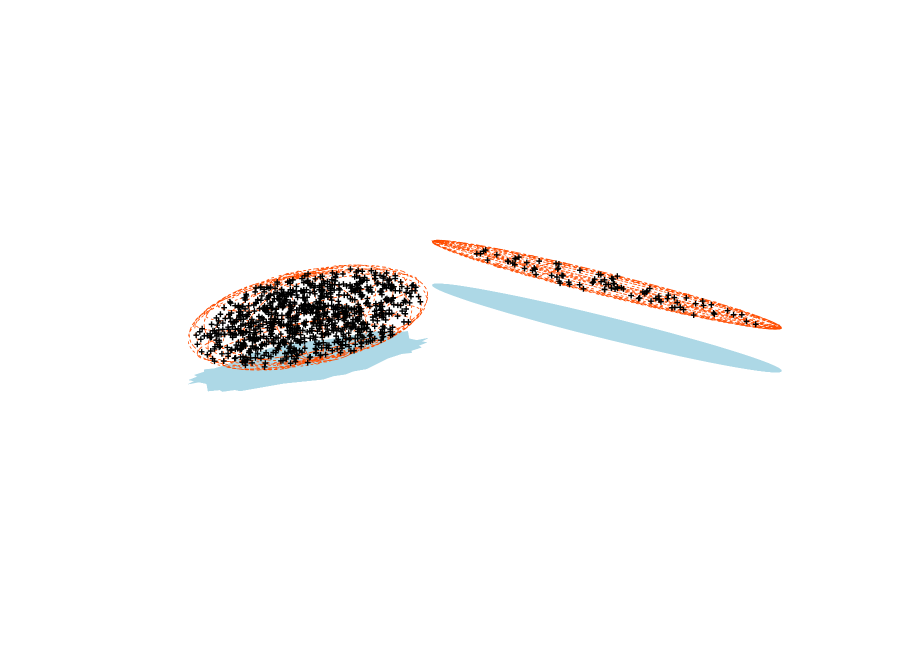
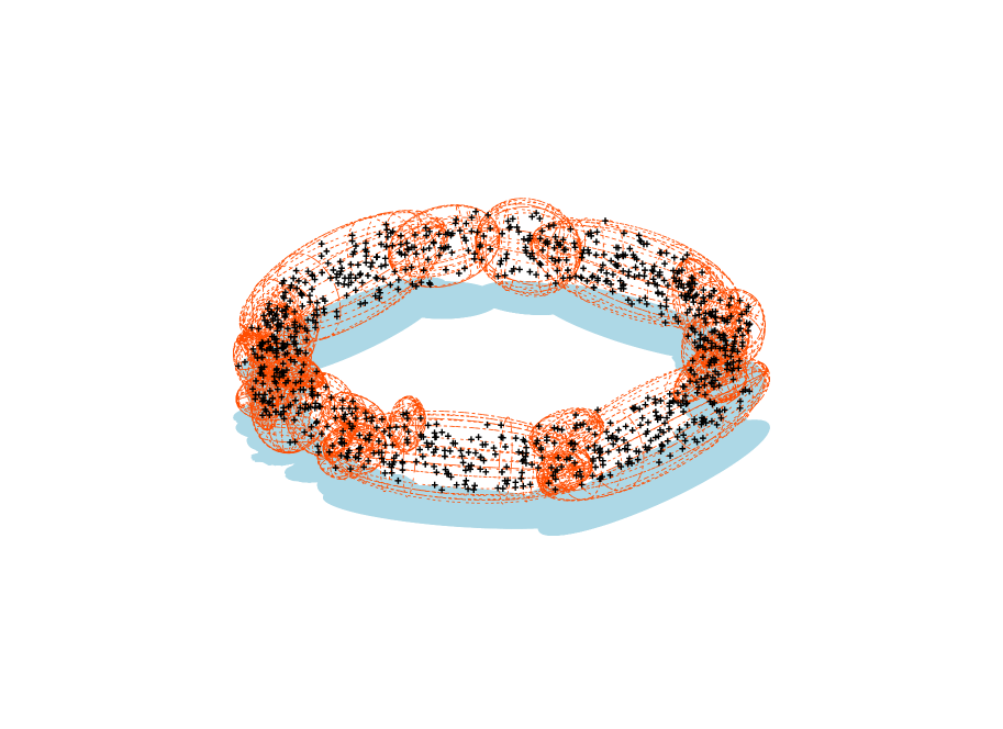
The approach outlined above allows maximum flexibility and sampling efficiency by breaking up a posterior mode resembling a Gaussian into relatively few ellipsoids, but a mode possesses a pronounced curving degeneracy into a relatively large number of small ‘overlapping’ ellipsoids. In Fig. 3 we show the results of applying Algorithm 1 to two different problems in three dimensions: in (a) the iso-likelihood surface consists of two non-overlapping ellipsoids, one of which contains correlations between the parameters; and in (b) the iso-likelihood surface is a torus. In each case, 1000 points were uniformly generated inside the iso-likelihood surface are used as the starting set $S$ in Algorithm 1. In case (a), Algorithm 1 correctly partitions the point set in two non-overlapping ellipsoids with $F(S)=1.1$, while in case (b) the point set is partitioned into 23 overlapping ellipsoids with $F(S)=1.2$.

In our nested sampling application, it is possible that the ellipsoids found by Algorithm 1 might not enclose the entire iso-likelihood contour, even though the sum of their volumes is constrained to exceed the prior volume $X$ This is because the ellipsoidal approximation to a region in the prior space might not be perfect. It might therefore be desirable to sample from a region with volume greater than the prior volume. This can easily be achieved by using $X/e$ as the desired minimum volume in Algorithm 1, where $X$ is the prior volume and $e$ the desired sampling efficiency ($1/e$ is the enlargement factor). We also note that if the desire sampling efficiency $e$ is set to be greater than unity, then the prior can be under-sampled. Indeed, setting $e>1$ can be useful if one is not interested in the evidence values, but wants only to have a general idea of the posterior structure in relatively few likelihood evaluations. We note that, regardless of the value of $e$, it is always ensured that the ellipsoids $E_{k}$ enclosing the subsets $S_{k}$ are always the bounding ellipsoids.

5.3 Sampling from overlapping ellipsoids

Once the ellipsoidal bounds have been constructed at some iteration of the nested sampling process, one must then draw a new point uniformly from the union of these ellipsoids, many of which may be overlapping. This is achieved using the method presented in FH08, which is summarised below for completeness.

Suppose at iteration $i$ of the nested sampling algorithm, one has $K$ ellipsoids $\{E_{k}\}$. One ellipsoid is then chosen with probability $p_{k}$ equal to its volume fraction

$$p_{k}=V(E_{k})/V_{\rm tot},$$ (23)

where $V_{\rm tot}=\sum_{k=1}^{K}V(E_{k})$. Samples are then drawn uniformly from the chosen ellipsoid until a sample is found for which the hard constraint $\mathcal{L}>\mathcal{L}_{i}$ is satisfied, where $\mathcal{L}_{i}$ is the lowest-likelihood value among all the active points at that iteration. There is, of course, a possibility that the chosen ellipsoid overlaps with one or more other ellipsoids. In order to take an account of this possibility, we find the number of ellipsoids, $n_{e}$, in which the sample lies and only accept the sample with probability $1/n_{e}$. This provides a consistent sampling procedure in all cases.

5.4 Decreasing the number of active points

For highly multimodal problems, the nested sampling algorithm would require a large number $N$ of active points to ensure that all the modes are detected. This would consequently result in very slow convergence of the algorithm. In such cases, it would be desirable to decrease the number of active points as the algorithm proceeds to higher likelihood levels, since the number of isolated regions in the iso-likelihood surface is expected to decrease with increasing likelihood. modes Fortunately, nested sampling does not require the number of active points to remain constant, provided the fraction by which the prior volume is decreased after each iteration is adjusted accordingly. Without knowing anything about the posterior, we can use the largest evidence contribution that can be made by the remaining portion of the posterior at the $i^{\rm th}$ iteration $\Delta{\mathcal{Z}}_{i}=\mathcal{L}_{\rm max}X_{i}$, as the guide in reducing the number of active points by assuming that the change in $\Delta{\mathcal{Z}}$ is linear locally. We thus set the number of active points $N_{i}$ at the $i^{\rm th}$ iteration to be

$$N_{i}=N_{i-1}-N_{\rm min}\frac{\Delta{\mathcal{Z}}_{i-1}-\Delta{\mathcal{Z}}_{i}}{\Delta{\mathcal{Z}}_{i}-\mbox{tol}},$$ (24)

subject to the constraint $N_{\rm min}\leq N_{i}\leq N_{i-1}$, where $N_{\rm min}$ is the minimum number of active points allowed and tol is the tolerance on the final evidence used in the stopping criterion.

5.5 Parallelization

Even with the enlargement factor $e$ set to unity (see Section 5.2), the typical sampling efficiency obtained for most problems in astrophysics and particle physics is around 20–30 per cent for two main reasons. First, the ellipsoidal approximation to the iso-likelihood surface at any iteration is not perfect and there may be regions of the parameter space lying inside the union of the ellipsoids but outside the true iso-likelihood surface; samples falling in such regions will be rejected, resulting in a sampling efficiency less than unity. Second, if the number of ellipsoids at any given iteration is greater than one, then they may overlap, resulting in some samples with $\mathcal{L}>\mathcal{L}_{i}$ falling inside a region shared by $n_{e}$ ellipsoids; such points are accepted only with probability $1/n_{e}$, which consequently lowers the sampling efficiency. Since the sampling efficiency is typically less than unity, the MultiNest algorithm can be usefully (and easily) parallelized by, at each nested sampling iteration, drawing a potential replacement point on each of $N_{\rm CPU}$ processors, where $1/N_{\rm CPU}$ is an estimate of the sampling efficiency.

5.6 Identification of modes

As discussed in FH08, for multimodal posteriors it can prove useful to identify which samples ‘belong’ to which mode. There is inevitably some arbitrariness in this process, since modes of the posterior necessarily sit on top of some general ‘background’ in the probability distribution. Moreover, modes lying close to one another in the parameter space may only ‘separate out’ at relatively high likelihood levels. Nonetheless, for well-defined, ‘isolated’ modes, a reasonable estimate of the posterior mass that each contains (and hence the associated ‘local’ evidence) can be defined, together with the posterior parameter constraints associated with each mode. To perform such a calculation, once the nested sampling algorithm has progressed to a likelihood level such that (at least locally) the ‘footprint’ of the mode is well-defined, one needs to identify at each subsequent iteration those points in the active set belonging to that mode. The partitioning and ellipsoids construction algorithm described in Section 5.2 provides a much more efficient and reliable method for performing this identification, as compared with the methods employed in FH08.

At the beginning of the nested sampling process, all the active points are assigned to one ‘group’ $G_{1}$. As outlined above, at subsequent iterations, the set of $N$ active points is partitioned into $K$ subsets $\{S_{k}\}$ and their corresponding ellipsoids $\{E_{k}\}$ constructed. To perform mode identification, at each iteration, one of the subsets $S_{k}$ is then picked at random: its members become the first members of the ‘temporary set’ $\mathcal{T}$ and its associated ellipsoid $E_{k}$ becomes the first member of the set of ellipsoids $\mathcal{E}$. All the other ellipsoids $E_{k^{\prime}}$ ($k^{\prime}\neq k)$ are then checked for intersection with $E_{k}$ using an exact algorithm proposed by Alfano & Greer (2003). Any ellipsoid found to intersect with $E_{k}$ is itself added to ${\cal E}$ and the members of the corresponding subset $S_{k}$ are added to $\mathcal{T}$. The set ${\cal E}$ (and consequently the set $\mathcal{T}$) is then iteratively built up by adding to it any ellipsoid not in ${\cal E}$ that intersects with any of those already in ${\cal E}$, until no more ellipsoids can be added. Once this is completed, if no more ellipsoids remain then all the points in $\mathcal{T}$ are (re)assigned to $G_{1}$, a new active point is drawn from the union of the ellipsoids $\{E_{k}\}$ (and also assigned to $G_{1}$) and the nested sampling process proceeds to its next iteration.

If, however, there remain ellipsoids $\{E_{k}\}$ not belonging to ${\cal E}$, then this indicates the presence of (at least) two isolated regions contained within the iso-likelihood surface. In this event, the points in $\mathcal{T}$ are (re)assigned to the group $G_{2}$ and the remaining active points are (re)assigned to the group $G_{3}$. The original group $G_{1}$ then contains only the inactive points generated up to this nested sampling iteration and is not modified further. The group $G_{3}$ is then analysed in a similar manner to see if can be split further (into $G_{3}$ and $G_{4}$), and the process continued until no further splitting is possible. Thus, in this case, one is left with an ‘inactive’ group $G_{1}$ and a collection of ‘active’ groups $G_{2}$, $G_{3}$, …. A new active point is then drawn from the union of the ellipsoids $\{E_{k}\}$, and assigned to the appropriate active group, and the nested sampling process proceeds to its next iteration.

At subsequent nested sampling iterations, each of the active groups present at that iteration is analysed in the same manner to see if it can be split. If so, then the active points in that group are (re)assigned to new active groups generated as above, and the original group becomes inactive, retaining only those of its points that are inactive. In order to minimize the computational cost, we take advantage of the fact that the ellipsoids created by Algorithm 1 can only get smaller in later iterations. Hence, within each active group, if two ellipsoids are found not to intersect at some iteration, they are not checked for intersection in later iterations. This makes the computational expense involved in separating out the modes negligible.

At the end of the nested sampling process, one thus obtains a set of inactive groups and a set of active groups, which between them partition the full set of (inactive and active) sample points generated. It is worth noting that, as the nested sampling process reaches higher likelihood levels, the number of active points in any particular active group may dwindle to zero, but such a group is still considered active since it remains unsplit at the end of the nested sampling run. Each active groups is then promoted to a ‘mode’, resulting in a set of $L$ (say) such modes $\{M_{l}\}$.

As a concrete example, consider the two-dimensional illustration shown in Fig. 4, in which the solid circles denote active points at the nested sampling iteration $i=i_{2}$, and the open circles are the inactive points at this stage.

Figure 4: Cartoon illustrating the assignment of points to groups; see text for details. The iso-likelihood contours $\mathcal{L}=\mathcal{L}_{i_{1}}$ and $\mathcal{L}=\mathcal{L}_{i_{2}}$ are shown as the dashed lines and dotted lines respectively. The solid circles denote active points at the nested sampling iteration $i=i_{2}$, and the open circles are the inactive points at this stage.

In this illustration, the first group $G_{1}$ remains unsplit until iteration $i=i_{1}$ of the nested sampling process, at which stage it is split into $G_{2}$, $G_{3}$ and $G_{4}$. The group $G_{3}$ then remains unsplit until iteration $i=i_{2}$, when it is split into $G_{5}$, $G_{6}$ and $G_{7}$. The group $G_{4}$ remains unsplit until iteration $i=i_{2}$, when it is split into $G_{8}$ and $G_{9}$. The group $G_{2}$ remains unsplit at iteration $i=i_{2}$ but the number of active points it contains has fallen to zero, since it is a low-lying region of the likelihood function. Thus, at the iteration $i=i_{2}$, the inactive groups are $G_{1}$, $G_{3}$ and $G_{4}$, and the active groups are $G_{2},G_{5},G_{6},G_{7},G_{8}$ and $G_{6}$. If (say) all of the latter collection of groups were to remain active until the end of the nested sampling process, each would then be promoted to a mode according to $M_{1}=G_{2}$, $M_{2}=G_{5}$, $M_{3}=G_{6},\cdots,M_{6}=G_{9}$.

5.7 Evaluating ‘local’ evidences

The reliable identification of isolated modes $\{M_{l}\}$ allows one to evaluate the local evidence associated with each mode much more efficiently and robustly than the methods presented in FH08. Suppose the $l^{\rm th}$ mode $M_{l}$ contains the points $\{\textbf{{u}}_{j}\}$ $(j=1,\cdots,n_{l})$. In the simplest approach, the local evidence of this mode is given by

$$\mathcal{Z}_{l}=\sum_{j=1}^{n_{l}}\mathcal{L}_{j}w_{j},$$ (25)

where (as in Eq. 8) $w_{j}=X_{M}/N$ for each active point in $M_{l}$, and for each inactive points $w_{j}=\tfrac{1}{2}(X_{i-1}-X_{i+1})$, in which $i$ is the nested sampling iteration at which the inactive point was discarded. In a similar manner, the posterior inferences resulting from the $l^{\rm th}$ mode are obtained by weighting each point in $M_{l}$ by $p_{j}=\mathcal{L}_{j}w_{j}/Z_{l}$.

As outlined in FH08, however, there remain some problems with this approach for modes that are sufficiently close to one another in the parameter space that they are only identified as isolated regions once the algorithm has proceeded to likelihood values somewhat larger than the value at which the modes actually separate. The ‘local’ evidence of each mode will then be underestimated by Eq. 25. In such cases, this problem can be overcome by also making use of the points contained in the inactive groups at the end of the nested sampling process, as follows.

For each mode $M_{l}$, expression Eq. 25 for the local evidence is replaced by

$$\mathcal{Z}_{l}=\sum_{j=1}^{n_{l}}\mathcal{L}_{j}w_{j}+\sum_{g}\mathcal{L}_{g}w_{g}\alpha^{(l)}_{g},$$ (26)

where the additional summation over $g$ includes all the points in the inactive groups, the weight $w_{g}=\tfrac{1}{2}(X_{i-1}-X_{i+1})$, where $i$ is the nested sampling iteration in which the $g^{\rm th}$ point was discarded, and the additional factors $\alpha^{(l)}_{g}$ are calculated as set out below. Similarly, posterior inferences from the $l^{\rm th}$ mode are obtained by weighting each point in $M_{l}$ by $p_{j}=\mathcal{L}_{j}w_{j}/Z_{l}$ and each point in the inactive groups by $p_{g}=\mathcal{L}_{g}w_{g}\alpha^{(l)}_{g}/Z_{l}$.

The factors $\alpha^{(l)}_{g}$ can be determined in a number of ways. The most straightforward approach is essentially to reverse the process illustrated in Fig. 4, as follows. Each mode $M_{l}$ is simply an active group $G$ that has been renamed. Moreover, one can identify the inactive group $G^{\prime}$ that split to form $G$ at the nested sampling iteration $i$. All points in the inactive group $G^{\prime}$ are then assigned the factor

$$\alpha_{g}^{(l)}=\frac{n^{(A)}_{G}(i)}{n^{(A)}_{G^{\prime}}(i)},$$ (27)

where $n^{(A)}_{G}(i)$ is the number of active points in $G$ at nested sampling iteration $i$, and similarly for $n^{(A)}_{G^{\prime}}(i)$. Now, the group $G^{\prime}$ may itself have been formed when an inactive group $G^{\prime\prime}$ split at an eariler nested sampling iteration $i^{\prime}<i$, in which case all the points in $G^{\prime\prime}$ are assigned the factor

$$\alpha_{g}^{(l)}=\frac{n^{(A)}_{G}(i)}{n^{(A)}_{G^{\prime}}(i)}\frac{n^{(A)}_{G^{\prime}}(i^{\prime})}{n^{(A)}_{G^{\prime\prime}}(i^{\prime})}.$$ (28)

The process is continued until the recursion terminates. Finally, all points in inactive groups not already assigned have $\alpha_{g}^{(l)}=0$.

As a concrete example, consider $M_{2}=G_{5}$ in Fig. 4. In this case, the factors assigned to the members of all the inactive groups $G_{1}$, $G_{3}$ and $G_{4}$ are

$$\alpha^{(2)}_{g}=\begin{cases}{\displaystyle\frac{n^{(A)}_{G_{5}}(i_{2})}{n^{(A)}_{G_{3}}(i_{2})}_{\phantom{\int}}}&\mbox{for $g\in G_{3}$}\\ {\displaystyle\frac{n^{(A)}_{G_{5}}(i_{2})}{n^{(A)}_{G_{3}}(i_{2})}\frac{n^{(A)}_{G_{3}}(i_{1})}{n^{(A)}_{G_{1}}(i_{1})}_{\phantom{\int}}}&\mbox{for $g\in G_{1}$}\\ 0&\mbox{for $g\in G_{4}$}\end{cases}$$ (29)

It is easy to check that the general prescription (Eqs. 27 and 28) ensures that

$$\sum_{l=1}^{L}\mathcal{Z}_{l}=\mathcal{Z},$$ (30)

i.e. the sum of the local evidences for each mode is equal to the global evidence. An alternative method for setting the factors $\alpha^{(l)}_{g}$, for which Eq. 30 again holds, is to use a mixture model to analyse the full set of points (active and inactive) produced, as outlined in Appendix A.

6 Applications

In this section we apply the MultiNest algorithm described above to two toy problems to demonstrate that it indeed calculates the Bayesian evidence and makes posterior inferences accurately and efficiently. These toy examples are chosen to have features that resemble those that can occur in real inference problems in astro- and particle physics.

6.1 Toy model 1: egg-box likelihood

We first demonstrate the application of MultiNest to a highly multimodal two-dimensional problem, for which the likelihood resembles an egg-box. The un-normalized likelihood is defined as

$$\mathcal{L}(\theta_{1},\theta_{2})=\exp\displaystyle\left[2+\cos\left(\frac{\theta_{1}}{2}\right)\cos\left(\frac{\theta_{2}}{2}\right)\right]^{5},$$ (31)

and we assume a uniform prior $\mathcal{U}(0,10\pi)$ for both $\theta_{1}$ and $\theta_{2}$.

\psfrag{x}{$x$}\psfrag{y}{$y$}\psfrag{z}{$\log(\mathcal{L})$}\includegraphics[width=433.62pt]{FIGS/eggbox.eps}

\psfrag{x}{$x$}\psfrag{y}{$y$}\psfrag{z}{$\log(\mathcal{L})$}\includegraphics[width=433.62pt]{FIGS/eggbox_results.eps}

Figure 5: Toy model 1: (a) two-dimensional plot of the likelihood function defined in Eq. 31; (b) dots denoting the points with the lowest likelihood at successive iterations of the MultiNest algorithm. Different colours denote points assigned to different isolated modes as the algorithm progresses.

A plot of the log-likelihood is shown in Fig. 5 and the the prior ranges are chosen such that some of the modes are truncated. Hence, although only two-dimensional, this toy example is a particularly challenging problem, not only for mode identification but also for evaluating the local evidence of each mode accurately. Indeed, even obtaining posterior samples efficiently from such a distribution can present a challenge for standard Metropolis–Hastings MCMC samplers. We note that distributions of this sort can occur in astronomical object detection applications (see FH08).

Owing to the highly multimodal nature of this problem, we use 2000 active points. The results obtained with MultiNest are illustrated in Fig. 5, in which the dots show the points with the lowest likelihood at successive iterations of the nested sampling process, and different colours indicate points assigned to different isolated modes as the algorithm progresses. MultiNest required $\sim 30,000$ likelihood evaluations and evaluated the global log-evidence value to be $235.86\pm 0.06$, which compares favourably with the log-evidence value of $235.88$ obtained through numerical integration on a fine grid. The local log-evidence values of each mode, calculated through numerical integration on a fine grid (denoted as ‘true $\log(\mathcal{Z})$’) and using MultiNest are listed in Table 1. We see that there is good agreement between the two estimates.

Mode	true local $\log(\mathcal{Z})$	MultiNest local $\log(\mathcal{Z})$
1	$233.33$	$233.20\pm 0.08$
2	$233.33$	$233.10\pm 0.06$
3	$233.33$	$233.48\pm 0.05$
4	$233.33$	$233.43\pm 0.05$
5	$233.33$	$233.65\pm 0.05$
6	$233.33$	$233.27\pm 0.05$
7	$233.33$	$233.14\pm 0.06$
8	$233.33$	$233.81\pm 0.04$
9	$232.64$	$232.65\pm 0.12$
10	$232.64$	$232.43\pm 0.16$
11	$232.64$	$232.11\pm 0.14$
12	$232.64$	$232.44\pm 0.11$
13	$232.64$	$232.68\pm 0.11$
14	$232.64$	$232.84\pm 0.09$
15	$232.64$	$233.02\pm 0.09$
16	$232.64$	$231.65\pm 0.29$
17	$231.94$	$231.49\pm 0.27$
18	$231.94$	$230.46\pm 0.36$

Table 1: The local log-evidence values of each mode for the toy model 1, described in Section 6.1, calculated through numerical integration on a fine grid (the ‘true $\log(\mathcal{Z})$’) and using the MultiNest algorithm.

6.2 Toy model 2: Gaussian shells likelihood

We now illustrate the capabilities of our MultiNest in sampling from a posterior containing multiple modes with pronounced (curving) degeneracies, and extend our analysis to parameters spaces of high dimension.

Figure 6: Toy model 2: (a) two-dimensional plot of the likelihood function defined in Eqs. (32) and (33); (b) dots denoting the points with the lowest likelihood at successive iterations of the MultiNest algorithm. Different colours denote points assigned to different isolated modes as the algorithm progresses.

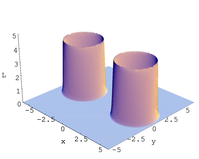
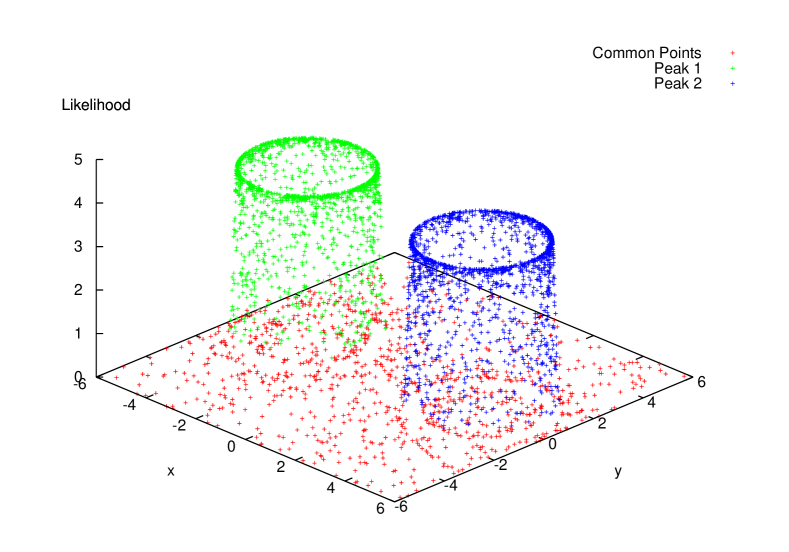
Our toy problem here is the same one used in FH08 and Allanach & Lester (2007). The likelihood function in this model is defined as,

$$\mathcal{L}(\mn@boldsymbol{\theta})={\rm circ}(\mn@boldsymbol{\theta};\mn@boldsymbol{c}_{1},r_{1},w_{1})+{\rm circ}(\mn@boldsymbol{\theta};\mn@boldsymbol{c}_{2},r_{2},w_{2}),$$ (32)

where

$${\rm circ}(\mn@boldsymbol{\theta};\mn@boldsymbol{c},r,w)=\frac{1}{\sqrt{2\pi w^{2}}}\exp\left[-\frac{(\left|\mn@boldsymbol{\theta}-\mn@boldsymbol{c}\right|-r)^{2}}{2w^{2}}\right].$$ (33)

In two dimensions, this toy distribution represents two well separated rings, centred on the points $\mn@boldsymbol{c}_{1}$ and $\mn@boldsymbol{c}_{2}$ respectively, each of radius $r$ and with a Gaussian radial profile of width $w$ (see Fig. 6). With a sufficiently small $w$ value, this distribution is representative of the likelihood functions one might encounter in analysing forthcoming particle physics experiments in the context of beyond-the-Standard-Model paradigms; in such models the bulk of the probability lies within thin sheets or hypersurfaces through the full parameter space.

We investigate the above distribution up to a $30$-dimensional parameter space $\mathbf{\Theta}$ with MultiNest. In all cases, the centres of the two rings are separated by $7$ units in the parameter space, and we take $w_{1}=w_{2}=0.1$ and $r_{1}=r_{2}=2$. We make $r_{1}$ and $r_{2}$ equal, since in higher dimensions any slight difference between these two values would result in a vast difference between the volumes occupied by the rings and consequently the ring with the smaller $r$ value would occupy a vanishingly small fraction of the total probability volume, making its detection almost impossible. It should also be noted that setting $w=0.1$ means the rings have an extremely narrow Gaussian profile and hence they represent an ‘optimally difficult’ problem for our ellipsoidal nested sampling algorithm, since many tiny ellipsoids are required to obtain a sufficiently accurate representation of the iso-likelihood surfaces. For the two-dimensional case, with the parameters described above, the likelihood is shown in Fig. 6.

	Analytical		MultiNest
$D$	log$(\mathcal{Z})$	local log$(\mathcal{Z})$	log$(\mathcal{Z})$	local log$(\mathcal{Z}_{1})$	local log$(\mathcal{Z}_{2})$
$2$	$-1.75$	$-2.44$	$-1.72\pm 0.05$	$-2.28\pm 0.08$	$-2.56\pm 0.08$
$5$	$-5.67$	$-6.36$	$-5.75\pm 0.08$	$-6.34\pm 0.10$	$-6.57\pm 0.11$
$10$	$-14.59$	$-15.28$	$-14.69\pm 0.12$	$-15.41\pm 0.15$	$-15.36\pm 0.15$
$20$	$-36.09$	$-36.78$	$-35.93\pm 0.19$	$-37.13\pm 0.23$	$-36.28\pm 0.22$
$30$	$-60.13$	$-60.82$	$-59.94\pm 0.24$	$-60.70\pm 0.30$	$-60.57\pm 0.32$

Table 2: The true and estimated global and local $\log(\mathcal{Z})$ for toy model 2, as a function of the dimensions $D$ of the parameter space, using MultiNest.

In analysing this problem using the methods presented in FH08, we showed that the sampling efficiency dropped significantly with increasing dimensionality, with the efficiency being less than 2 per cent in 10 dimensions, with almost $600,000$ likelihood evaluations required to estimate the evidence to the required accuracy. Using 1000 active points in MultiNest, we list the evaluated and analytical evidence values in Table 2. The total number of likelihood evaluations and the sampling efficiencies are listed in Table 3. For comparison, we also list the number of likelihood evaluations and the sampling efficiencies with the ellipsoidal nested sampling method proposed in FH08. One sees that MultiNest requires an order of magnitude fewer likelihood evaluations than the method of FH08. In fact, the relative computational cost of MultiNest is even less than this comparison suggests, since it no longer performs an eigen-analysis at each iteration, as discussed in Section 5.2. Indeed, for this toy problem discussed, the EM partitioning algorithm discussed in Section 5.2 was on average called only once per 1000 iterations of the MultiNest algorithm.

	from FH08		MultiNest
$D$	$N_{\rm like}$	Efficiency	$N_{\rm like}$	Efficiency
$2$	$27,658$	$15.98\%$	$7,370$	$70.77\%$
$5$	$69,094$	$9.57\%$	$17,967$	$51.02\%$
$10$	$579,208$	$1.82\%$	$52,901$	$34.28\%$
$20$	$43,093,230$	$0.05\%$	$255,092$	$15.49\%$
$30$			$753,789$	$8.39\%$

Table 3: The number of likelihood evaluations and sampling efficiency for the ellipsoidal nested sampling algorithm of FH08 and MultiNest, when applied to toy model 2 as a function of the dimension $D$ of the parameter space.

7 Cosmological parameter estimation and model selection

Likelihood functions resembling those used in our toy models do occur in real inference problems in astro- and particle physics, such as object detection in astronomy (see e.g. Hobson & McLachlan 2003; FH08) and analysis of beyond-the-Standard-Model theories in particle physics phenomenology (see e.g. Feroz et al. 2008). Nonetheless, not all likelihood functions are as challenging and it is important to demonstrate that MultiNest is more efficient (and certainly no less so) than standard Metropolis–Hastings MCMC sampling even in more straightforward inference problems.

An important area of inference in astrophysics is that of cosmological parameter estimation and model selection, for which the likelihood functions are usually quite benign, often resembling a single, broad multivariate Gaussian in the allowed parameter space. Therefore, in this section, we apply the MultiNest algorithm to analyse two related extensions of the standard cosmology model: non-flat spatial curvature and a varying equation of state of dark energy.

The complete set of cosmological parameters and the ranges of the uniform priors assumed for them are given in Table 4, where the parameters have their usual meanings. With $\Omega_{\rm k}=0$ and $w=-1$ this model then represents the ‘vanilla’ $\Lambda$CDM cosmology. In addition, mirroring the recent analysis of the WMAP 5-year (WMAP5) data (Dunkley et al., 2008), a Sunyaev-Zel’dovich amplitude is introduced, with a uniform prior in the range $[0,2]$. We have chosen three basic sets of data: CMB observations alone; CMB plus the Hubble Space Telescope (HST) constraint on $H_{0}$ (Freedman et al., 2001); and CMB plus large scale structure (LSS) constraints on the matter power spectrum derived from the luminous red galaxy (LRG) subset of the Sloan Digital Sky Survey (SDSS; Tegmark et al. 2006; Tegmark et al. 2004) and the two degree field survey (2dF; Cole et al. 2005). In addition, for the dark energy analysis we include distance measures from supernovae Ia data (Kowalski et al., 2008). The CMB data comprises WMAP5 observations (Hinshaw et al., 2008) + higher resolution datasets from the Arcminute Cosmology Bolometer Array (ACBAR; Reichardt et al. 2008) + the Cosmic Background Imager (CBI; Readhead et al. 2004; Sievers J. L. et al. 2007; CBI Supplementary Data 2006) + Balloon Observations of Millimetric Extragalactic Radiation and Geophysics (BOOMERanG; Piacentini et al. 2006; Jones et al. 2006; Montroy et al. 2006).

Observations of the first CMB acoustic peak cannot in themselves constrain the spatial curvature $\Omega_{\rm k}$. This could be constrained using angular scale of the first acoustic peak coupled with a knowledge of the distance to the last scattering surface, but the latter is a function of the entire expansion history of the universe and so there is a significant degeneracy between $\Omega_{\rm k}$ and the Hubble parameter $H(z)$. This dependence, often termed the ‘geometric degeneracy’, can be broken, however, since measurements at different redshifts can constrain a sufficiently different functions of $\Omega_{\rm k}$ and $H$. Thus, the combination of CMB data with measurements of the acoustic peak structure in the matter power spectrum derived from large scale structure surveys such as the LRG subset of Sloan can place much tighter constraints on curvature than with either alone (see e.g. Eisenstein et al. 2005; Tegmark et al. 2006; Komatsu et al. 2008).

Inflation generically predicts a flat universe (Guth, 1981). The tightest current constraint suggests $\Omega_{\rm k}\approx 10^{-2}$, whereas inflation lasting over 60 e-folds would produce flatness at the level of $10^{-5}$ (Komatsu et al., 2008). Thus, at present, the data is not capable of refuting or confirming such an inflationary picture. From a Bayesian point of view, however, one can still assess whether the data currently prefers the inclusion of such a physical parameter.

$0.018$	$\leq\Omega_{\rm b}h^{2}\leq$	$0.032$
$0.04$	$\leq\Omega_{\rm cdm}h^{2}\leq$	$0.16$
$0.98$	$\leq\Theta\leq$	$1.1$
$0.01$	$\leq\tau\leq$	$0.5$
$-0.1$	$\leq\Omega_{\rm k}\leq$	$0.1$
$-1.5$	$\leq w\leq$	$-0.5$
$0.8$	$\leq n_{\rm s}\leq$	$1.2$
$2.6$	$\leq\log[10^{10}A_{\rm s}]\leq$	$4.2$

Table 4: Cosmological parameters and uniform priors ranges for the vanilla $\Lambda$CDM model, plus spatial curvature $\Omega_{\rm k}$ and dark energy equation of state parameter $w$.

The algorithmic parameters of MultiNest were appropriately chosen given our a priori knowledge of the uni-modal form of typical cosmological posteriors, the dimensionality of the problem and some empirical testing. The number of active points was set to $N=400$ and a sampling efficiency $e$ of 0.3 means that MPI parallelisation across 4 CPUs is optimal (with a further 4 openmp threads per MPI CPU used by CAMB’s multithreading facility). This represents a relatively modest computational investment. All of the inferences obtained in this section required between 40,000 and 50,000 likelihood evaluations.

7.1 Results: spatial curvature

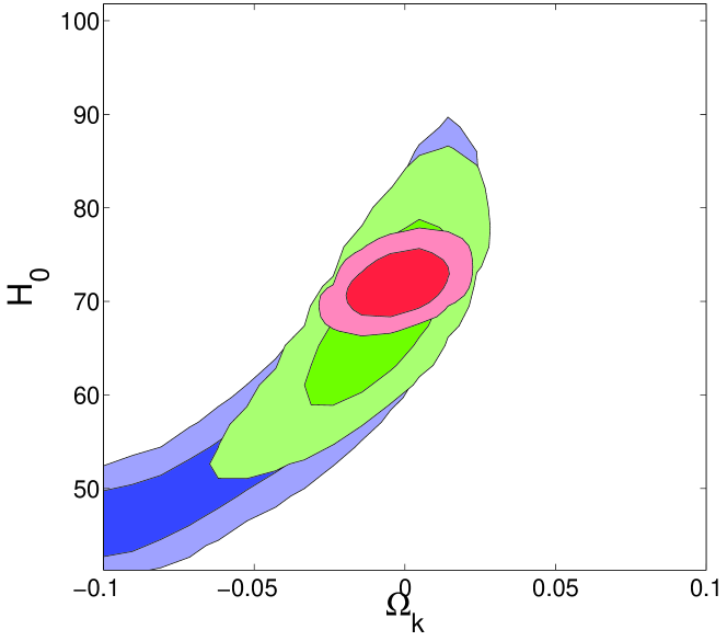
Fig. 7. illustrates the progressively tighter constraints placed on $\Omega_{\rm k}$ and $H_{0}$ produced by combining CMB data with other cosmological probes of large scale structure. The geometric degeneracy is clearly unbroken with CMB data alone, but the independent constraints on $H_{0}$ by HST are seen to tighten the constraint somewhat. Including LSS data, specifically the LRG data, markedly reduces the uncertainty on the curvature so that at 1-$\sigma$ we can limit the curvature range to $-0.043\leq\Omega_{\rm k}\leq 0.004$. The asymmetry of this constraint leaves a larger negative tail of $\Omega_{\rm k}$ resulting in a mean value that is only slightly closed. However, even these most stringent parameter constraints available, we see no statistically significant deviation from a spatially flat universe. The Bayesian evidence, in penalising excessive model complexity should tell us whether relaxing the constraint on flatness is preferred by the data. Our results (Table 5) very clearly rule out the necessity for such an addition in anything other than with CMB data alone. This implies that the inclusion of spatial curvature is an unnecessary complication in cosmological model building, given the currently available data.

Figure 7: Breaking of the ‘geometric’ degeneracy in CMB data (blue) via the addition of HST (green) and large scale structure data (red).

Dataset $\backslash$ Model	vanilla + $\Omega_{\rm k}$	vanilla + $\Omega_{\rm k}$ + $w$
CMB alone	$-0.29\pm 0.27$	-
CMB + HST	$-1.56\pm 0.27$	-
ALL	$-2.92\pm 0.27$	$-1.29\pm 0.27$

Table 5: Differences of $\log$ evidences for both models and the three datasets described in the text.[Negative (Positive) values represent lower (higher) preference for the parameterisation change]

7.2 Results: varying equation of state of dark energy

The properties of the largest universal density component are still largely unknown, yet such a component seems crucial for the universe to be spatially flat. It has thus been argued by some (Wright 2006 & Tegmark et al. 2006) that it is inappropriate to assume spatial flatness when attempting to vary the properties of the dark energy component beyond those of a simple cosmological constant. Here we allow for the variation of the dark energy equation of state parameter $w$. We will therefore proceed by placing joint constraints on both $w$ and $\Omega_{\rm k}$, as performed in Komatsu et al. (2008). Once again we encounter a serious degeneracy, this time between $\Omega_{\rm k}$ and $w$. With the geometric degeneracy, combining cosmological observations of the universe at different redshifts was sufficient to break the dependence, but when dark energy is dynamical we must use at least a third, independent data set. In this analysis, we have therefore included distance measures from type Ia supernovae observations (Kowalski et al., 2008). Using this combination of data produces impressively tight constraints on both $w$ and $\Omega_{\rm k}$; indeed the resulting constraints on the spatial curvature are tighter than those obtained in the previous section, for which $w$ was held constant at $w=-1$. This is primarily due to the near orthogonality of the constraints provided by supernovae and the CMB. Once again we find little evidence to support a departure from the basic vanilla cosmology (see Table 5). To within estimated uncertainty, the Bayesian evidence is at least one log unit greater for a flat universe with dark energy in the form of a cosmological constant.

Figure 8: Joint constraints on universal geometry $\Omega_{\rm k}$ and the equation of state of dark energy $w$ using WMAP5 + HST + LSS + supernovae data.

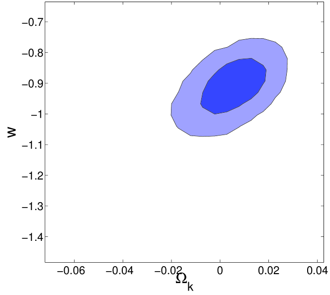
7.3 Comparison of MultiNest and MCMC ‘quick look’ parameter constraints

The above results are in good agreement with those found by Komatsu et al. (2008) using more traditional MCMC methods, and indicate that MultiNest has produced reliable inferences, both in terms of the estimated evidence values and the derived posterior parameter constraints. It is often the case, however, that cosmologists wish only to obtain a broad idea of the posterior distribution of parameters, using short MCMC chains and hence relatively few likelihood evaluations. In this section, we show that the MultiNest algorithm can also perform this task by setting the number of active points, $N$, to a smaller value.

In order to illustrate this functionality, we analyse the WMAP5 CMB data-set in the context of the vanilla $\Lambda$CDM cosmology using both MultiNest and the publicly available CosmoMC Lewis & Bridle (2002) package, which uses an MCMC sampler based on a tailored version of the Metropolis–Hastings method. We imposed uniform priors on all the parameters. The prior ranges for $\Omega_{\rm b}h^{2},\Omega_{\rm cdm}h^{2},\Theta$, and $\tau$ is listed in Table 4. In addition, $n_{\rm s}$ was allowed to vary between 0.8 and 1.2, $\log(10^{10}A_{\rm s})$ between 2.6 and 4.2 and the Sunyaev–Zel’dovich amplitude between 0 and 2.

To facilitate later comparisons, we first obtained an accurate determination of the posterior distribution using the traditional method by running CosmoMC to produce 4 long MCMC chains. The Gelman–Rubin statistic $R$ returned by CosmoMC indicated that the chains had converged to within $R\approx 1.1$ after about 6000 steps per chain, resulting in $\sim$ 24,000 likelihood evaluations. To be certain of determining the ‘true’ posterior to high accuracy, we then ran the MCMC chains for a further 6,000 samples per chain, resulting in a total of 48,000 likelihood evaluations, at which point the convergence statistic was $R\approx 1.05$.

As stated above, however, one often wishes to obtain only a ‘quick-and-dirty’ estimate of the posterior in the first stages of the data analysis. As might be typical of such analyses, we ran CosmoMC again using 4 MCMC chains, but with only 800 steps per chain, resulting in a total of 3,200 likelihood evaluations. As a comparison, we also ran the MultiNest algorithm using only 50 active points and with the sampling efficiency $e$ set to unity; this required a total of 3,100 likelihood evaluations. In Fig. 9, we plot the 1-D marginalized posteriors for derived from the two analyses, together with the results of the longer CosmoMC analysis described above. It is clear from these plots that both the MultiNest and MCMC ‘quick-look’ results compare well with the ‘true’ posterior obtained from the more costly rigorous analysis.

\psfrag{xl1}{$\Omega_{\rm b}h^{2}$}\psfrag{xl2}{$\Omega_{\rm cdm}h^{2}$}\psfrag{xl3}{$\Theta$}\psfrag{xl4}{$\tau$}\psfrag{xl5}{$n_{\rm s}$}\psfrag{xl6}{$\log(10^{10}A_{\rm s})$}\includegraphics[width=433.62pt]{FIGS/mcmc_multinest.eps}

Figure 9: 1-D marginalized posteriors for the flat-$\Lambda$CDM cosmology obtained with: CosmoMC using 48,000 likelihood evaluations (solid black); CosmoMC using 3,200 likelihood evaluations (dotted pink); and MultiNest using 3,100 likelihood evaluations (dashed blue).

8 Discussion and conclusions

We have described a highly efficient Bayesian inference tool, called MultiNest, which we have now made freely available for academic purposes as a plugin that is easily incorporated into the CosmoMC software. On challenging toy models that resemble real inference problems in astro- and particle physics, we have demonstrated that MultiNest produces reliable estimates of the evidence, and its uncertainty, and accurate posterior inferences from distributions with multiple modes and pronounced curving degeneracies in high dimensions. We have also demonstrated in cosmological inference problems that MultiNest produces accurate parameter constraints on similar time scales to standard MCMC methods and, with negligible extra computational effort, also yields very accurate Bayesian evidences for model selection. As a cosmological application we have considered two extensions of the basic vanilla $\Lambda$CDM cosmology: non-zero spatial curvature and a varying equation of state of dark energy. Both extensions are determined to be unnecessary for the modelling of existing data via the evidence criterion, confirming that with the advent of five years of WMAP observations the data is still satisfied by a $\Lambda$CDM cosmology.

As a guide for potential users, we conclude by noting that the MultiNest algorithm is controlled by two main parameters: (i) the number of active points $N$; and (ii) the maximum efficiency $e$ (see Section 5.2). These values can be chosen quite easily as outlined below. First, $N$ should be large enough that, in the initial sampling from the full prior space, there is a high probability that at least one point lies in the ‘basin of attraction’ of each mode of the posterior. In later iterations, active points will then tend to populate these modes. It should be remembered, of course, that $N$ must always exceed the dimensionality $D$ of the parameter space. Also, in order to calculate the evidence accurately, $N$ should be sufficiently large so that all the regions of the parameter space are sampled adequately. For parameter estimation only, one can use far fewer active points. For cosmological data analysis, we found $400$ and $50$ active points to be adequate for evidence evaluation and parameter estimation respectively. The parameter $e$ controls the sampling volume at each iteration, which is equal to the sum of the volumes of the ellipsoids enclosing the active point set. For parameter estimation problems, $e$ should be set to $1$ to obtain maximum efficiency without undersampling or to a lower value if one wants to get a general idea of the posterior very quickly. For evidence evaluation in cosmology, we found setting $e\sim 0.3$ ensures an accurate evidence value.

Appendix A Local evidence evaluation using a Gaussian mixture model

As mentioned in Section 5.7, an alternative method for determining the local evidence and posterior constraints associated with each identified mode $M_{l}$ is to analyse the full set of samples using a mixture model. In what follows, we assume that the modes of the ‘implied’ posterior $\mathcal{P}(\textbf{{u}})$ in the unit hypercube space are each well described by a multivariate Gaussian, leading to a Gaussian mixture model, but the model for the mode shape can be easily changed to another distribution.

Let us assume that, at the end of the nested sampling process, the full set of ${\cal N}$ (inactive and active) points obtained is $\{\textbf{{u}}_{1},\textbf{{u}}_{2},\cdots,\textbf{{u}}_{\cal N}\}$ and $L$ modes $M_{1},M_{2},\cdots,M_{L}$ modes have been identified. The basic goal of the method is to assign an extra factor $\alpha^{(l)}_{j}$ to every point ($j=1$ to $\mathcal{N}$), so that the estimate (Eq. 26) for the local evidence associated with the mode $M_{l}$ is replaced by

$$\mathcal{Z}_{l}=\sum_{j=1}^{\mathcal{N}}\mathcal{L}_{j}w_{j}\alpha^{(l)}_{j},$$ (34)

where the weights $w_{j}$ for the inactive and active points are the same as those used in Eq. 26. Similarly, posterior inferences from the mode $M_{l}$ are obtained by weighting every point ($j=1$ to $\mathcal{N}$) by $p_{j}=\mathcal{L}_{j}w_{j}\alpha^{(l)}_{j}/Z_{l}$.

The factors $\alpha^{(l)}_{j}$ are determined by modelling each mode $M_{l}$ as a multivariate Gaussian with ‘normalised amplitude’ $A_{l}$, mean $\mn@boldsymbol{\mu}_{l}$ and covariance matrix $\mathbf{C}_{l}$, such that

$$\mathcal{P}(\textbf{{u}})\propto\sum_{l=1}^{L}A_{l}G(\textbf{{u}};\mn@boldsymbol{\mu}_{l},\mathbf{C}_{l}),$$ (35)

where the Gaussian unit-volume $G(\textbf{{u}};\mn@boldsymbol{\mu}_{l},\mathbf{C}_{l})$ is given by

$$G(\textbf{{u}};\mn@boldsymbol{\mu}_{l},\mathbf{\Theta}_{l})=\frac{1}{(2\pi)^{\frac{{\rm D}}{2}}|\mathbf{C}_{l}|^{\frac{1}{2}}}\exp\displaystyle\left[-{\textstyle\frac{1}{2}}(\textbf{{u}}-\mn@boldsymbol{\mu}_{l})^{\rm T}\mathbf{C}_{l}^{-1}(\textbf{{u}}-\mn@boldsymbol{\mu}_{l})\right],$$ (36)

and the values of the parameters $\mathbf{\Theta}\equiv(\{A_{l}\},\{\mn@boldsymbol{\mu}_{l}\},\{\mathbf{C}_{l}\})$ are to be determined from the sample points $\{\textbf{{u}}_{j}\}$. Since the scaling in Eq. 35 is arbitrary, it is convenient to set $\sum_{l=1}^{L}A_{l}=1$.

For a given set of parameter values $\mathbf{\Theta}$, our required factors are

$$\alpha^{(l)}_{j}(\mathbf{\Theta}) = \Pr(M_{l}|\textbf{{u}}_{j},\mathbf{\Theta})$$ (37)

$$= \frac{\Pr(\textbf{{u}}_{j}|M_{l},\mathbf{\Theta})\Pr(M_{l}|\mathbf{\Theta})}{\sum_{l=1}^{L}\Pr(\textbf{{u}}_{j}|M_{l},\mathbf{\Theta})\Pr(M_{l}|\mathbf{\Theta})}$$

$$= \frac{A_{l}G(\textbf{{u}};\mn@boldsymbol{\mu}_{l},\mathbf{C}_{l})}{\sum_{l=1}^{L}A_{l}G(\textbf{{u}};\mn@boldsymbol{\mu}_{l},\mathbf{C}_{l})}.$$

Our approach is to optimise the parameters $\mathbf{\Theta}$, and hence determine the factors $\alpha^{(l)}_{j}(\mathbf{\Theta})$, using an expectation-maximization (EM) algorithm. The algorithm is initialized by setting

$$\alpha^{(l)}_{j}=\begin{cases}1&\mbox{if $\textbf{{u}}_{j}\in M_{l}$}\\ 0&\mbox{otherwise}\end{cases}$$ (38)

and calculating the initial values of each $Z_{l}$ using Eq. 34. In the M-step of the algorithm one then obtains the maximum-likelihood estimates $\hat{\mathbf{\Theta}}$ of the parameters. These are easily derived (see e.g.  Dempster et al. (1977)) to be

$$\widehat{A}_{l} = \frac{n_{l}}{n}$$ (39)

$$\widehat{\mn@boldsymbol{\mu}}_{l} = \frac{1}{n_{l}}\sum_{j=1}^{\mathcal{N}}\alpha^{(l)}_{j}\tilde{\textbf{{u}}}_{j}$$ (40)

$$\widehat{\mathbf{C}}_{l} = \frac{1}{n_{l}}\sum_{j=1}^{\mathcal{N}}\alpha^{(l)}_{j}(\tilde{\textbf{{u}}}_{j}-\widehat{\mn@boldsymbol{\mu}}_{l})(\tilde{\textbf{{u}}}_{j}-\widehat{\mn@boldsymbol{\mu}}_{l})^{\rm T},$$ (41)

where $n_{l}=\sum_{j=1}^{\mathcal{N}}\alpha^{(l)}_{j}$, $n=\sum_{l=1}^{L}n_{l}$ and $\tilde{\textbf{{u}}}_{j}=\textbf{{u}}_{j}L_{j}w_{j}/Z_{l}$ are the locally posterior-weighted sample points. In the subsequent E-step of the algorithm on then updates the $\alpha^{(l)}_{j}$ values using Eq. 37 and updates $Z_{l}$ using Eq. 34. We further impose the constraint that $\alpha^{(l)}_{j}=0$ if $\textbf{{u}}_{j}\notin M_{l}$ and its likelihood $\mathcal{L}_{j}$ is greater than the lowest likelihood of the points in $M_{l}$. The EM algorithm is then iterated to convergence.

References

- Allanach & Lester (2007) Allanach B. C., Lester C. G., , 2007, Sampling using a ‘bank’ of clues
- Bassett et al. (2004) Bassett B. A., Corasaniti P. S., Kunz M., 2004, Astrophys. J., 617, L1
- Beltrán et al. (2005) Beltrán M., García-Bellido J., Lesgourgues J., Liddle A. R., Slosar A., 2005, Phys.Rev.D, 71, 063532
- Bridges et al. (2006) Bridges M., Lasenby A. N., Hobson M. P., 2006, MNRAS, 369, 1123
- CBI Supplementary Data (2006) CBI Supplementary Data 2006
- Cole et al. (2005) Cole S., et al., 2005, Mon. Not. Roy. Astron. Soc., 362, 505
- Dempster et al. (1977) Dempster A. P., Laird N. M., Rubin D. B., 1977, Journal of the Royal Statistical Society. Series B (Methodological), 39, 1
- Dunkley et al. (2008) Dunkley J., Komatsu E., Nolta M. R., Spergel D. N., Larson D., Hinshaw G., Page L., Bennett C. L., Gold B., Jarosik N., Weiland J. L., Halpern M., Hill R. S., Kogut A., Limon M., Meyer S. S., Tucker G. S., Wollack E., Wright E. L., 2008, ArXiv e-prints, 803
- Eisenstein et al. (2005) Eisenstein D. J., Zehavi I., Hogg D. W., Scoccimarro R., Blanton M. R., Nichol R. C., Scranton R., Seo H.-J., Tegmark M., Zheng Z., Anderson S. F., 2005, ApJ, 633, 560
- Feroz et al. (2008) Feroz F., Allanach B. C., Hobson M., AbdusSalam S. S., Trotta R., Weber A. M., , 2008, Bayesian Selection of sign(mu) within mSUGRA in Global Fits Including WMAP5 Results
- Feroz & Hobson (2008) Feroz F., Hobson M. P., 2008, MNRAS, 384, 449
- Freedman et al. (2001) Freedman W. L., Madore B. F., Gibson B. K., Ferrarese L., Kelson D. D., Sakai S., Mould J. R., Kennicutt Jr. R. C., Ford H. C., Graham J. A., Huchra J. P., Hughes S. M. G., Illingworth G. D., Macri L. M., Stetson P. B., 2001, ApJ, 553, 47
- Guth (1981) Guth A. H., 1981, Phys.Rev.D, 23, 347
- Hinshaw et al. (2008) Hinshaw G., Weiland J. L., Hill R. S., Odegard N., Larson D., Bennett C. L., Dunkley J., Gold B., 2008, ArXiv e-prints, 803
- Hobson et al. (2002) Hobson M. P., Bridle S. L., Lahav O., 2002, MNRAS, 335, 377
- Hobson & McLachlan (2003) Hobson M. P., McLachlan C., 2003, MNRAS, 338, 765
- Jones et al. (2006) Jones W. C., et al., 2006, ApJ, 647, 823
- Komatsu et al. (2008) Komatsu E., Dunkley J., Nolta M. R., Bennett C. L., Gold B., Hinshaw G., Jarosik N., Larson D., Limon M., Page L., Spergel D. N., Halpern M., Hill R. S., Kogut A., Meyer S. S., Tucker G. S., Weiland J. L., Wollack E., Wright E. L., 2008, ArXiv e-prints, 803
- Kowalski et al. (2008) Kowalski M., et al., 2008
- Lewis & Bridle (2002) Lewis A., Bridle S., 2002, Phys.Rev.D, 66, 103511
- Liddle (2007) Liddle A. R., 2007, ArXiv Astrophysics e-prints
- Lu et al. (2007) Lu L., Choi Y.-K., Wang W., Kim M.-S., 2007, Computer Graphics Forum, 26, 329
- Mackay (2003) Mackay D. J. C., 2003, Information Theory, Inference and Learning Algorithms. Information Theory, Inference and Learning Algorithms, by David J. C. MacKay, pp. 640. ISBN 0521642981. Cambridge, UK: Cambridge University Press, October 2003.
- Marshall et al. (2003) Marshall P. J., Hobson M. P., Slosar A., 2003, MNRAS, 346, 489
- Montroy et al. (2006) Montroy T. E., et al., 2006, ApJ, 647, 813
- Mukherjee et al. (2006) Mukherjee P., Parkinson D., Liddle A. R., 2006, ApJ, 638, L51
- Niarchou et al. (2004) Niarchou A., Jaffe A. H., Pogosian L., 2004, Phys.Rev.D, 69, 063515
- Ó Ruanaidh & Fitzgerald (1996) Ó Ruanaidh J., Fitzgerald W., 1996, Numerical Bayesian Methods Applied to Signal Processing. Springer Verlag:New York
- Piacentini et al. (2006) Piacentini F., et al., 2006, ApJ, 647, 833
- Readhead et al. (2004) Readhead A. C. S., Mason B. S., Contaldi C. R., Pearson T. J., Bond J. R., Myers S. T., Padin S., Sievers J. L., Cartwright J. K., 2004, ApJ, 609, 498
- Reichardt et al. (2008) Reichardt C. L., et al., 2008
- Shaw et al. (2007) Shaw J. R., Bridges M., Hobson M. P., 2007, MNRAS, 378, 1365
- Sievers J. L. et al. (2007) Sievers J. L. et al. 2007, Astrophys. J., 660, 976
- Skilling (2004) Skilling J., 2004, in Fischer R., Preuss R., Toussaint U. V., eds, American Institute of Physics Conference Series Nested Sampling. pp 395–405
- Slosar A. et al. (2003) Slosar A. et al. 2003, MNRAS, 341, L29
- Tegmark et al. (2006) Tegmark M., Eisenstein D., Strauss M., Weinberg D., Blanton M., Frieman J., Fukugita M., Gunn J., Hamilton A., Knapp G., Nichol R., Ostriker J., 2006, ArXiv Astrophysics e-prints
- Tegmark et al. (2004) Tegmark M., et al., 2004, Astrophys. J., 606, 702
- Tegmark et al. (2006) Tegmark M., et al., 2006, Phys. Rev., D74, 123507
- Trotta (2007) Trotta R., 2007, MNRAS, 378, 72
- Wright (2006) Wright E. L., 2006, ArXiv Astrophysics e-prints