Doping a Mott insulator with orbital degrees of freedom

Abstract

We study the effects of hole doping on one-dimensional Mott insulators with orbital degrees of freedom. We describe the system in terms of a generalized $t-J$ model. At a specific point in parameter space the model becomes integrable in analogy to the one-band supersymmetric $t-J$ model. We use the Bethe ansatz to derive a set of nonlinear integral equations which allow us to study the thermodynamics exactly. Moving away from this special point in parameter space we use the density-matrix renormalization group applied to transfer matrices to study the evolution of various phases of the undoped system with doping and temperature. Finally, we study a one-dimensional version of a realistic model for cubic titanates which includes the anisotropy of the orbital sector due to Hund’s coupling. We find a transition from a phase with antiferromagnetically correlated spins to a phase where the spins are fully ferromagnetically polarized, a strong tendency towards phase separation at large Hund’s coupling, as well as the possibility of an instability towards triplet superconductivity.

I Introduction

In many transition metal oxides, different orbital configurations are close in energy or even degenerate. Small changes in temperature or pressure can therefore lead to a complete rearrangement of the electron clouds which in turn also strongly influences the magnetic and the transport properties. Such orbital degrees of freedom play an important role, for example, in the manganites, titanates, vanadates, and ruthenates.Tokura and Nagaosa (2000); Khaliullin (2005) Quite common for these transition metal oxides is the perovskite crystal structure where each transition metal ion is surrounded by an octahedron of oxygen ions. For a $3d$ transition metal ion, the cubic crystal field then splits the fivefold orbital degeneracy into threefold degenerate $t_{2g}$ orbitals and twofold degenerate $e_{g}$ orbitals. Here we want to concentrate first on the case where we have one electron per site in the $t_{2g}$ orbitals with the $e_{g}$ orbitals being inactive (fully occupied or empty). Because the onsite Coulomb interactions are large the system is a Mott insulator in this case. The strongly anisotropic shape of the $t_{2g}$ orbitals means that the direction an electron can move to create a virtually excited state depends on the orbital it is sitting in. More precisely, hopping is only possible between orbitals of the same kind, and along a particular crystal axis only two out of the three $t_{2g}$ orbitals are active. This can lead to a (dynamical) lowering of the effective dimensionality of the system in various ways: Conventional orbital ordering can restrict the hopping to one-dimensional chains which can then show typical one-dimensional phenomena like a Haldane gap Lee et al. (2006) or a Peierls effect.Khomskii and Mizokawa (2005) More unconventional mechanisms like an orbital-driven Peierls effectUlrich et al. (2003); Sirker and Khaliullin (2003) or spin-orbital nematic states Khaliullin (2005) might also render the system quasi one dimensional. In the latter cases, however, there will still be a twofold orbital degeneracy. A simple Hamiltonian capturing the essential physics is then given by

$$H=2J\sum_{j}\left(\boldsymbol{S}_{j}\boldsymbol{S}_{j+1}+x\right)\left(\boldsymbol{\tau}_{j}\boldsymbol{\tau}_{j+1}+y\right)$$ (1)

where $\boldsymbol{S}$ is an $S=1/2$ spin operator and $\boldsymbol{\tau}$ a $\tau=1/2$ orbital pseudospin describing the occupation of the two degenerate orbitals active along the chain direction. $J=4t^{2}/U$ is the magnetic superexchange constant, $t$ the hopping amplitude, $U$ the onsite Coulomb repulsion, and $x,y$ real numbers often treated as free parameters. From a microscopic derivation of the effective model (1) it follows, however, that $x,y$ are determined by the Hund’s rule coupling $J_{H}$ with $x=y=1/4$ corresponding to $J_{H}=0$. In addition, such a derivation shows that a finite Hund’s coupling does not only modify $x,y$ but also leads to an $xxz$-type anisotropy of the orbital sector.Khaliullin (2005) This anisotropy is neglected in (1). We will come back to the relation between this simple model and more realistic models in section V.

The spin-orbital model (1) has been intensely studied Li et al. (1998); Yamashita et al. (1998); Pati and Singh (2000); Frischmuth et al. (1999); Itoi et al. (2000); Azaria et al. (2000); Pati et al. (1998); Sirker (2004) and a number of different phases depending on $x,y$ have been identified (see e.g. Refs. Itoi et al., 2000, Chen et al., 2007). In general, the model has a $SU(2)\times SU(2)$ symmetry and exhibits an additional $Z_{2}$ symmetry, interchanging spin and orbital degrees of freedom, if $x=y$. At the special point $x=y=1/4$ the symmetry is enlarged even further to $SU(4)$. This has to do with the fact that at this point the Hamiltonian is just a permutation operator of states on neighboring sites. The model therefore becomes a version of the Uimin-Sutherland model and is integrable by Bethe ansatz.Sutherland (1975)

In this work we want to study the effects of hole doping on the spin-orbital model (1). Because states with more than one electron per site are effectively forbidden due to the strong Coulomb repulsion $U$, hole doping of the Mott insulator (1) naturally leads us to a generalized $t-J$ model

$$H=t\sum_{j}\sum_{\sigma,\tau}\mathcal{P}\left\{c^{\dagger}_{j,\sigma,\tau}c_{j+1,\sigma,\tau}+h.c.\right\}\mathcal{P}+2J\sum_{j}\left\{\left(\boldsymbol{S}_{j}\boldsymbol{S}_{j+1}+x\right)\left(\boldsymbol{\tau}_{j}\boldsymbol{\tau}_{j+1}+yn_{j}n_{j+1}\right)-\frac{n_{j}n_{j+1}}{4}\right\}\;.$$ (2)

Here $\mathcal{P}$ projects out the doubly occupied states, $\sigma$ is the spin, and $\tau$ the orbital index. As for the one-band $t-J$ model it turns out that there is a special point in parameter space $J/t=2$, $x=y=1/4$ where the model is integrable by Bethe ansatz. Again, the symmetry is enlarged at this point to $SU(4|1)$ (graded $SU(5)$ symmetry), the Hamiltonian is a permutation operator of states on neighboring sites and falls into the Uimin-Sutherland class of models.

In Sec. II we will investigate the thermodynamics of this model at the integrable point with the help of the Bethe ansatz and the quantum transfer matrix approach. Details of the Bethe ansatz calculation are presented in appendix A. In Sec. III we briefly introduce the density-matrix renormalization group applied to transfer matrices (TMRG) which we will use to study the thermodynamics of model (2) numerically away from the integrable point. We will test the accuracy of this method by comparing with exact results at the integrable point. In section IV we will use the TMRG algorithm to study the evolution of various phases of the undoped model (1) with doping and temperature. In Sec. V we finally consider a one-dimensional version of a realistic model for cubic titanates which includes the $xxz$-type anisotropy of the orbital sector due to Hund’s coupling. We investigate the phase transitions, possible tendencies towards phase separation as well as superconducting instabilities as a function of the strength of Hund’s coupling. In Sec. VI we present a short summary and our conclusions.

II The integrable model

The integrable $SU(4|1)$ model (2) with $J/t=2$, $x=y=1/4$ has already been studied by Schlottmann. Schlottmann (1992, 1993) He derived the Bethe ansatz equations and studied the ground state properties as well as the elementary excitations. Kawakami later then derived the critical exponents of various correlation functions. Kawakami (1993) Here we want to concentrate on the thermodynamics of this model. Based on the quantum transfer matrix approach we derive a set of nonlinear integral equations (NLIE) which then are evaluated numerically to obtain various thermodynamic quantities. Details about the derivation of the NLIE are given in appendix A.

Our results for the thermodynamics in the low temperature limit can be connected to Schlottmann’s and Kawakami’s results for the elementary excitations using conformal field theory. The $SU(4)$ spin-orbital model, i.e., model (2) with $n=1$, is known to belong to the universality class of the $SU(4)_{1}$ Wess-Zumino-Witten (WZW) models,Affleck (1986); Itoi et al. (2000) so that the central charge $c_{so}=3$. Similar to the one-band supersymmetric $t-J$ model we expect that the critical theory for the hole-doped model is a semidirect product of the spin-orbital and the charge part so that the free energy at low temperatures is given by

$$f=e_{0}-\frac{\pi}{6}\left(\frac{c_{so}}{v_{so}}+\frac{c_{c}}{v_{c}}\right)T^{2}\;.$$ (3)

Here $e_{0}$ is the ground state energy which can be calculated by Bethe ansatzSchlottmann (1993), $v_{so}$ ($v_{c}$) are the velocities of the elementary spin-orbital (charge) excitations, respectively, and $c_{c}=1$ the central charge of the charge sector.

In Fig. 1 we show the specific heat as a function of temperature for various fillings.

Figure 1: (color online) Specific heat for the integrable model (2) with $J/t=2$ and $x=y=1/4$ calculated by BA. The left inset shows the spin-orbital ($v_{so}$) and the charge velocity ($v_{c}$) as a function of particle density $n$. The right inset compares the BA results (solid lines) with the low temperature asymptotics obtained from CFT (dashed lines), see Eq. (4).

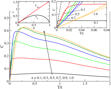
According to Eq. (3) the specific heat at low temperatures is linear and determined by the elementary charge and spin-orbital excitations

$$C=-T\frac{\partial^{2}f}{\partial T^{2}}=\frac{\pi}{3}\left(\frac{c_{so}}{v_{so}}+\frac{c_{c}}{v_{c}}\right)T\;.$$ (4)

As shown in the left inset of Fig. 1 the velocities of the charge and spin-orbital excitations go to zero for $n\to 0$ so that the slope of $C$ diverges in this limit. For $n\to 1$, on the other hand, only $v_{c}\to 0$ whereas $v_{so}\to J\pi/4$. This also leads to a diverging slope, however, the charge excitations are quickly exhausted so that this behavior is only visible at very low temperatures. At higher temperatures (but still $T\ll t$) the slope then crosses over to the value given by the spin-orbital excitations only. Finally, for $n=1$, we have $C=2T$ in the whole conformal regime. In the low temperature limit, the BA results which we obtained by the quantum transfer matrix approach indeed agree perfectly with the CFT result (4) using the velocities determined according to Ref. Schlottmann, 1993 (see right inset of Fig. 1).

The magnetic susceptibility $\chi_{s}$ as a function of temperature is shown in Fig. 2.

Figure 2: (color online) Magnetic susceptibility $\chi_{s}$ for the integrable model. The dashed lines denote the zero temperature limit according to CFT.

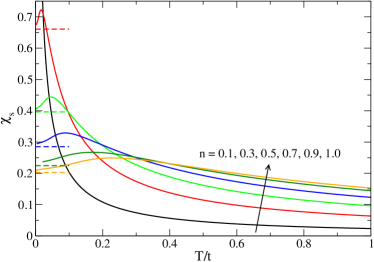
From CFT we expect $\chi_{s}=1/\pi v_{so}$ at zero temperature. Because $v_{so}$ vanishes for $n\to 0$, the magnetic susceptibility diverges in this limit. For $n=1$, on the other hand, we have $v_{so}=J\pi/4$ so that $\chi_{s}=2/\pi^{2}$. Note, however, that logarithmic corrections are expected at low temperatures similar to the Heisenberg chain. Therefore the susceptibility will approach the zero temperature limit predicted by CFT with infinite slope. This explains why even at the lowest temperatures shown in Fig. 2 the susceptibility curves obtained by BA still deviate significantly from the zero temperature limit. In Fig. 3 we show the compressibility $\chi_{c}$ for various densities.

Figure 3: (color online) Compressibility $\chi_{c}$ for the integrable model. The lines denote the zero temperature limit according to CFT. The inset shows the dressed charge as a function of density.

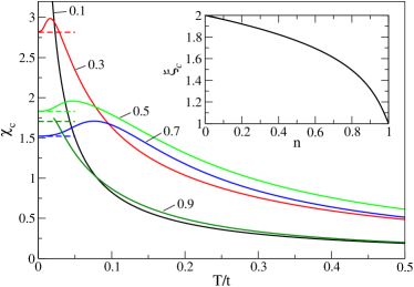
For the compressibility CFT predicts $\chi_{c}=K_{c}/(\pi v_{c})$ where $K_{c}$ is the Luttinger parameter of the charge sector. Using the BA we can calculate the so called dressed chargeKawakami (1993); Frahm and Schadschneider (1993); Izergin et al. (1989), $\xi_{c}(Q)$, which is related to the Luttinger parameter by $K_{c}=\xi_{c}(Q)^{2}$. The dressed charge as a function of density is shown in the inset of Fig. 3. Because the charge velocity vanishes for $n\to 0$ and $n\to 1$ (see Fig. 1) we have a diverging compressibility in both limits. In addition, we notice that even at intermediate densities the compressibility is large indicating that the integrable point is not that far from a phase separated state. In general, phase separation is promoted by an increasing ratio of $J/t$ as is well known in the $SU(2)$ $t-J$ model.Ogata et al. (1991); Hellberg and Mele (1991) We will come back to this point in Sec. IV.

Finally, we want to consider the transport properties of the integrable model at zero temperature. We can write the real part of the conductivity at zero momentum as $\sigma^{\prime}(\omega)=2\pi D\delta(\omega)+\sigma_{\mbox{reg}}(\omega)$ where $D$ is the Drude weight and $\sigma_{\mbox{reg}}(\omega)$ the regular part. With the help of conformal field theory and Bethe ansatz we find

$$D=\frac{K_{c}v_{c}}{2\pi}=\frac{\xi_{c}^{2}(Q)v_{c}}{2\pi}\;.$$ (5)

Thus, the Drude weight follows directly from the dressed charge shown in the inset Fig. 3 and the charge velocity shown in the left inset of Fig. 1 and is depicted in Fig. 4.

Figure 4: (color online) Drude weight $D$ for the supersymmetric point $J=2t$ (black solid line) and for $J=0$ (red dashed line), respectively. In the insets the regions of small and large densities are shown in detail.

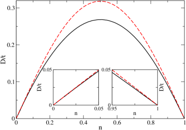
$D$ vanishes for $n\to 0$ where the number of charge carriers vanishes, and for $n\to 1$ where the Mott gap opens up. Quite surprisingly, the Drude weight for the supersymmetric point appears to be symmetric around $n=1/2$ although the Hamiltonian (2) does not possess such a symmetry. To understand this behavior it is instructive to study in addition the Drude weight for $J=0$. In this case only the kinetic energy part of (2) remains. Then the spin and orbital indices do not matter and due to the projection operators the model becomes equivalent to a one-band, spinless fermion model. Note that the Mott gap at $n=1$ is therefore still incorporated. The Drude weight can now be calculated from

$$e(\Phi)-e(0)=D\Phi^{2}/N^{2}+\mathcal{O}(N^{-3})$$ (6)

with $e$ being the ground state energy per site, and $\Phi$ a field describing a twist in the boundary conditions, $c_{j+N}=\text{e}^{i\Phi}c_{j}$. We find

$$D(J=0)=\frac{t}{\pi}\sin{\pi n}$$ (7)

which is shown as dashed curve in Fig. 4. Now the Drude weight is indeed symmetric around $n=1/2$ because the spinless fermion model is particle-hole symmetric. The comparison with the supersymmetric case near $n\sim 0$ in the left inset of Fig. 4 shows that the Drude weights coincide in this limit. This is expected because the exchange interaction $J$ becomes irrelevant in the dilute limit. For $n\sim 1$ shown in the right inset of Fig. 4, on the other hand, we see that the two curves do not coincide. In this limit $J$ cannot be neglected. This means that $D$ for the supersymmetric case is not symmetric around $n=1/2$ but the deviations from this symmetry are very small. Similar observations have been made for the one-band supersymmetric $t-J$ model by Kawakami and Yang, Ref. Kawakami and Yang, 1991.

III Density-matrix renormalization group

The density-matrix renormalization group applied to transfer matrices (TMRG) is based on a mapping of a one-dimensional quantum system to a two-dimensional classical one by means of a Trotter-Suzuki decomposition. In the classical model one direction is spatial whereas the other corresponds to the inverse temperature. For the classical system a so called quantum transfer matrix (QTM) is defined which evolves along the spatial direction. At any non-zero temperature the QTM has the crucial property that its largest eigenvalue $\Lambda_{0}$ is separated from the other eigenvalues by a finite gap. The partition function of the system in the thermodynamic limit is therefore determined by $\Lambda_{0}$ only, allowing it to perform this limit exactly. The Trotter-Suzuki decomposition is discrete so that the transfer matrix has a finite number of sites or local Boltzmann weights $M$. The temperature is given by $T\sim(\epsilon M)^{-1}$ where $\epsilon$ is the discretization parameter used in the Trotter-Suzuki decomposition. The algorithm starts at some high-temperature value where $M$ is so small that the QTM can be diagonalized exactly. Using a standard infinite-size DMRG algorithm, sites are then added to the QTM leading to a successive lowering of the temperature. The TMRG algorithm is described in detail in Refs. I.Peschel et al., 1999, Glocke et al., 2008, Sirker and Klümper, 2002a and has been applied to a number of one-dimensional systems such as frustrated and dimerized spin chains,Klümper et al. (1999) the Kondo lattice model,Mutou et al. (1998) the $t-J$ chainSirker and Klümper (2002a, b) and ladderAmmon et al. (1999) as well as to the extended Hubbard model.Glocke et al. (2007)

To obtain insight into the physical properties of the doped spin-orbital model we will, in particular, be interested in the behavior of two-point correlation functions. At finite temperatures we expect that any two-point correlation function of a local operator $O(r)$ decays exponentially with distance $r$

$$\langle O(1)O(r)\rangle-\langle O(1)\rangle\langle O(r)\rangle=\sum_{n}M_{n}\text{e}^{-r/\xi_{n}}\text{e}^{ik_{n}r}\;.$$ (8)

Here $M_{n}$ is a matrix element, $\xi_{n}$ the correlation length, and $k_{n}$ the corresponding wave vector. Note, that in the asymptotic expansion (8) infinitely many correlation lengths appear. Within the TMRG algorithm, correlation lengths and corresponding wave vectors are determined by next-leading eigenvalues $\Lambda_{n}$ of the QTM

$$\xi_{n}^{-1}=\ln\left|\frac{\Lambda_{0}}{\Lambda_{n}}\right|\quad,\quad k_{n}=\arg\left(\frac{\Lambda_{n}}{\Lambda_{0}}\right)\;.$$ (9)

The long-distance behavior of the correlation function is then dominated by the correlation length $\xi_{\alpha}$ belonging to the largest eigenvalue $\Lambda_{\alpha}$ ($\alpha\neq 0$) with $M_{\alpha}\neq 0$.

Apart from spin-spin (orbital-orbital) $\langle\boldsymbol{S}(1)\boldsymbol{S}(r)\rangle$ ($\langle\boldsymbol{\tau}(1)\boldsymbol{\tau}(r)\rangle$) two-point correlation functions we are also interested in pair correlation functions to investigate possible superconducting instabilities. For the model (2) we can define the following singlet and triplet pair correlation functions

$$G_{tt}(r) = \langle c_{\uparrow a}(r+1)c_{\uparrow a}(r)c^{\dagger}_{\uparrow a}(2)c^{\dagger}_{\uparrow a}(1)\rangle$$

$$G_{ss}(r) = \langle c_{\uparrow a}(r+1)c_{\downarrow b}(r)c^{\dagger}_{\uparrow a}(2)c^{\dagger}_{\downarrow b}(1)\rangle$$ (10)

$$G_{ts}(r) = \langle c_{\uparrow a}(r+1)c_{\uparrow b}(r)c^{\dagger}_{\uparrow a}(2)c^{\dagger}_{\uparrow b}(1)\rangle$$

$$G_{st}(r) = \langle c_{\uparrow a}(r+1)c_{\downarrow a}(r)c^{\dagger}_{\uparrow a}(2)c^{\dagger}_{\downarrow a}(1)\rangle\;.$$

Here $a,b$ denote the $\tau^{z}$-component and $\uparrow,\downarrow$ the $S^{z}$-component. For each of these pair correlations an asymptotic expansion (8) exists and relation (9) can be used to numerically determine the corresponding leading correlation lengths.

The discrete Trotter parameter $\epsilon$ leads to a systematic error in the free energy of order $\epsilon^{2}$. In the calculations presented here we have chosen $\epsilon=0.05$ so that this error is expected to be of the order $10^{-3}-10^{-4}$. More important is the error due to the truncation of the Hilbert space in each DMRG step. This error is difficult to estimate but accumulates with each DMRG step finally leading to a breakdown of the numerics at low temperatures. In the calculation presented here we will keep $N=240-360$ states as basis for the truncated Hilbert space. To decide down to which temperatures the TMRG is reliable we show results for the free energy and density at the integrable point in Fig. 5.

Figure 5: (color online) (a): Free energy $f$ calculated by TMRG (symbols) with $N=360$ states kept compared to the exact solution (lines). The black circles (black solid lines) denote the result for $\mu=-1.7$, the red squares (red dashed lines) for $\mu=-1.9$, and the blue diamonds (blue dot-dashed lines) for $\mu=-2.5$, respectively. (b): Absolute error $|\Delta_{f}|$ of the TMRG results presented in (a). (c): TMRG results for the density compared to the exact solution with symbols and lines denoting the same chemical potentials as in (a). (d): Absolute error $|\Delta_{n}|$ of the TMRG results in (c).

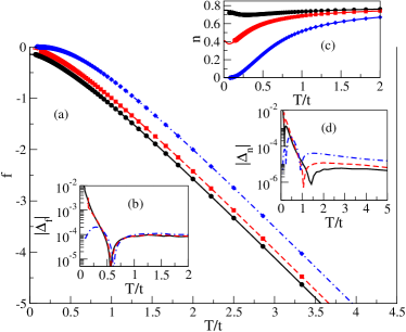
It is important to note, that we perform the numerical calculations in a grand canonical ensemble, i.e., we fix the chemical potential and not the particle density. In particular for small doping levels it is, however, possible to find a chemical potential so that the density depends only very weakly on temperature as shown in Fig. 5(c). Note that for $T\to\infty$ we always have $n\to 4/5$ because we have 5 states locally with one state corresponding to the empty site. The absolute errors in the free energies and in the densities stay smaller than $10^{-2}$ for temperatures down to $T/t\sim 0.1$ as shown in Fig. 5(b) and (d), respectively. This accuracy is completely sufficient to study the thermodynamic properties of model (2), and temperatures of the order $T/t\sim 0.1$ are low enough to identify the ground state as well.

IV The $xy$-model

In this section we want to investigate model (2) away from the integrable point. First, we want to demonstrate that the integrable point is indeed already close to a state with phase separation. While keeping $x=y=1/4$ we now set $J/t=3$ and show in Fig. 6 the density as a function of chemical potential for various temperatures.

Figure 6: (color online) The density $n$ as a function of chemical potential $\mu$ for different temperatures. Here $J/t=3$ and $x=y=1/4$. The lines are guides to the eye.

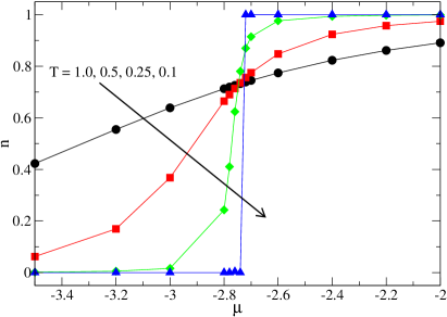
For $T/t\to 0$ the density is zero for $\mu<-2.73$ and equal to one otherwise. This means that the compressibility calculated at any fixed density is divergent and the ground state therefore phase separated. The reason for phase separation is obvious: For large $J/t$ the system tries to maximize its magnetic exchange energy which is achieved by separating the particles from the holes.

For all transition metal oxides we expect in general $J=4t^{2}/U<t$ which is equivalent to $4t<U$. Exact values for $J/t$ depend on the considered compound but values of $J/t\sim 0.3-0.5$ are typical. As a representative value we will concentrate in the following on $J/t=0.5$.

IV.1 The dimerized phase

For $x=y=1/2$ the undoped model is in a dimerized phase and spin and orbital excitations are gapped.Itoi et al. (2000); Sirker (2004) Spin-Peierls-type instabilities are a generic feature of systems with coupled spin and orbital degrees of freedom and have been investigated in more detail in Refs. Sirker and Khaliullin, 2003, Sirker et al., 2008. Here we want to study how dimer order and excitation gap evolve with doping. In Fig. 7 the magnetic susceptibility for various doping levels is shown.

Figure 7: (color online) Spin (orbital) susceptibility for $J/t=0.5$ and $x=y=1/2$ and different chemical potentials. Insets: (a) Corresponding densities as function of temperature. (b) Leading spin (orbital) dimer correlation length $\xi_{D}$.

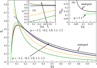
Note, that due to the $Z_{2}$ symmetry spin and orbital sectors are equivalent and spin and orbital susceptibility therefore identical. In the undoped case a spin gap $\Delta$ is clearly visible. In Ref. Sirker, 2004 this gap has been found to be of the order $\Delta=0.090\pm 0.005$. With increasing hole concentration the spin gap becomes smaller but is still detectable numerically at a chemical potential $\mu=1.0$ which corresponds to a density $n=0.85$ at low temperatures. For larger doping levels the spin excitations seem to become gapless so that the system apparently turns into a Luttinger liquid. The long-range dimer order, on the other hand, seems to break down immediately when holes are added to the system. In the case of algebraically decaying correlations at zero temperature we expect the corresponding correlation length to diverge as $\xi\sim 1/T$ whereas $\xi$ will diverge stronger than $1/T$ in the case of true long-range order. In inset (b) of Fig. 7 we therefore show the leading spin (orbital) dimer correlation length $\xi_{D}$ multiplied by $T$. In the undoped case the divergence of $T\xi_{D}$ indicates that the ground state has indeed long-range dimer order, whereas for a chemical potential $\mu=1.1$, corresponding to $n\sim 0.9$ at low temperatures, $T\xi_{D}$ is decreasing with temperature. Here we expect $\xi_{D}$ to stay finite so that $T\xi_{D}\to 0$ for $T\to 0$ in accord with the numerical data.

IV.2 Ferromagnetic/Antiferromagnetic-phase

Here we want to consider $J/t=0.5$ with $x=0.5$, $y=-0.5$ where the undoped model shows ferromagnetism in the spin sector and algebraically decaying antiferromagnetic correlations in the orbital sector.Itoi et al. (2000) As shown in inset (a) of Fig. 8 we find that the density for a chemical potential $\mu=-0.1$ is almost constant, $n\sim 0.84$, for temperatures $T\in[0,2]$. This allows us to compare the undoped model directly with this slightly doped case.

Figure 8: (color online) TMRG results for $J/t=0.5$ with $x=1/2$ and $y=-1/2$. Main figure: Spin susceptibility in the undoped case and for $\mu=-0.1$ as function of temperature. Insets: (a) For $\mu=-0.1$ the density $n\sim 0.84$ is almost independent of temperature. (b) Nearest-neighbor spin-spin and orbital-orbital expectation values for the undoped model and for $\mu=-0.1$ ($n\sim 0.84$). The circles on the $T=0$ axis denote $1/4$ and $-\ln 2+1/4$, respectively. (c) Charge compressibility for $\mu=-0.1$.

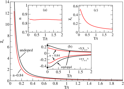
In the main figure the spin susceptibility $\chi_{s}$ as a function of temperature is shown. As expected, $\chi_{s}$ becomes suppressed with doping but still diverges for $T\to 0$ indicating long-range ferromagnetic order in both cases. In inset (b) of Fig. 8 the nearest-neighbor spin-spin and orbital-orbital expectation values are shown. In the undoped case $\langle\boldsymbol{S}_{i}\boldsymbol{S}_{i+1}\rangle\to 1/4$ for $T\to 0$ as expected for ferromagnetic order. When the spins order ferromagnetically, then, according to Hamiltonian (1), we have an effective antiferromagnetic coupling for the orbitals so that $\langle\boldsymbol{\tau}_{i}\boldsymbol{\tau}_{i+1}\rangle\to-\ln 2+1/4$ for $T\to 0$. This is the value for an antiferromagnetic Heisenberg chain known from Bethe ansatz. In the slightly doped case both the ferromagnetic spin and the antiferromagnetic orbital correlations become weaker. The charge compressibility shown in inset (c) of Fig. 8 is nonzero for $T\to 0$ indicating that the charge excitations are gapless.

This leads us to the question if the system has algebraically decaying pair correlations and if so, which one of the pair correlations defined in (III) dominates. In Fig. 9 we show some of the leading correlation lengths.

Figure 9: (color online) Leading correlation lengths for $J/t=0.5$, $x=1/2$, $y=-1/2$. The leading spin-spin correlation length is non-oscillating ($k=0$) whereas the orbital-orbital and the pair correlations show incommensurate oscillations at low temperatures as depicted in the inset.

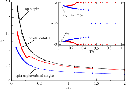
Dominant is the spin-spin correlation length with wave vector $k=0$ which diverges as $1/T$ indicative of the ferromagnetic order in the ground state.Takahashi (1986) Next, we find a correlation length which belongs to the asymptotic expansion of the orbital-orbital correlation function. Interestingly, the associated wave vector is given by $k=\pi$ for $T/t\gtrsim 0.28$ but becomes incommensurate at lower temperatures. At $T/t\sim 0.28$ the correlation length shows a cusp. The explanation for this cusp is as follows: In the asymptotic expansion (8) of the orbital-orbital correlation function we have two correlation lengths with wave vector $k=\pi$. At $T/t\sim 0.28$ these two correlation lengths cross and the oscillations of the now leading correlation length become incommensurate. For $T\to 0$ we find that $k\to\pm 2k_{F}=\pm\pi n\approx\pm 2.64$ for $n\sim 0.84$. So at $T=0$ the incommensurate oscillations just reflect the incommensurate filling of the system. Similar crossover phenomena in the leading correlation length at finite temperature have also been observed in the $xxz$ model in a magnetic field Klümper et al. (2001) and in the one-band $t-J$ model at incommensurate filling.Sirker and Klümper (2002a, b)

For the pair correlations defined in (III) we find that the spin triplet/orbital singlet correlation $G_{ts}$ has the largest correlation length $\xi_{ts}$. At low temperatures we find $\xi_{ts}\sim 1/T$ indicating that $G_{ts}$ will decay algebraically at zero temperature. The associated wave vector is given by $k_{ts}=0$ for $T/t\gtrsim 0.5$ but becomes incommensurate at lower temperatures. The numerical data seem to indicate that for $T\to 0$ the oscillations become commensurate again with $k_{ts}=\pi$. In the ground state this would mean that $G_{ts}(r)\sim(-1)^{r}/r^{x}$ with some critical exponent $x$.

In the ferromagnetic/antiferromagnetic-phase considered in this section a coupling between spin-orbital chains might therefore induce true long-range triplet superconductivity. Here triplet superconductivity arises from the coupling of the spins with the orbital pseudospins. The degenerate orbitals order antiferromagnetically leading to an effective ferromagnetic coupling for the spins.

V A one-dimensional version of a realistic model for cubic titanates

In recent years a lot of interest has focused on the Mott insulator LaTiO₃.Khaliullin and Maekawa (2000); Khaliullin (2005) Here the octahedron of oxygen ions surrounding each Ti³⁺ is nearly perfect. This opens up the possibility that the orbital degeneracy is not lifted by lattice distortions and that the orbitals act as additional quantum degrees of freedom. Starting from the ideal case of completely degenerate $t_{2g}$-orbitals one can derive a superexchange model similar to (1). Here the two orbitals represented by the orbital pseudospin $\boldsymbol{\tau}$ depend on the bond direction. Along the $c$-axis, for example, only the $t_{2g}$ levels of $xz$ and $yz$ symmetry are active and represented by $\boldsymbol{\tau}$, whereas $\boldsymbol{\tau}$ stands for the $xy$ and $xz$ orbital if the bond is along the $a$-axis. Having different orbital pairs active along each spatial direction necessarily frustrates the one-dimensional physics discussed in the previous sections of this paper and might lead to a liquid state with short range $SU(4)$-type correlations.Khaliullin and Maekawa (2000) Nevertheless, a directional, nematic state where the system makes full use of the orbital quantum fluctuations say along the $c$-axis with active $xz$ and $yz$ orbitals while the $xy$ orbital is empty, thus preventing orbital fluctuations in the other two directions, might be close in energy and could possibly be realized in LaTiO₃ under pressure.Khaliullin (2005) An example, where such orbital selection leading to a strongly directional spin-orbital state probably happens is YVO₃. In this system, however, we have an effective spin $S=1$.Ulrich et al. (2003); Sirker and Khaliullin (2003)

It is important to take the Hund’s rule splitting of the virtual excited states into account when deriving the superexchange Hamiltonian for LaTiO₃. This leads, in particular, to an $xxz$-type anisotropy of the orbital sector, i.e., contrary to (1) the Hamiltonian no longer has a $SU(2)\times SU(2)$ symmetry. If we consider the hole-doped case and add the hopping of the holes to the superexchange Hamiltonian for LaTiO₃ given in Ref. Khaliullin, 2005, we obtain again a $t-J$ type Hamiltonian which can be represented as

$$H = t\sum_{j}\sum_{\sigma,\tau}\mathcal{P}\left\{c^{\dagger}_{j,\sigma,\tau}c_{j+1,\sigma,\tau}+h.c.\right\}\mathcal{P}$$

$$+ 2J_{\mathit{eff}}\left[\left(\boldsymbol{S}_{j}\boldsymbol{S}_{j+1}+x\right)\left(\boldsymbol{\tau}_{j}\boldsymbol{\tau}_{j+1}+\delta\tau^{z}_{j}\tau^{z}_{j+1}+yn_{j}n_{j+1}\right)-\frac{z}{4}n_{j}n_{j+1}+\gamma\tau^{z}_{j}\tau^{z}_{j+1}\right]$$

with parameters

$$J_{\mathit{eff}}=\frac{J}{2}(r_{1}+r_{2})\quad,\quad x=\frac{1}{4}+\frac{1}{2}\frac{r_{1}-r_{2}}{r_{1}+r_{2}}$$

$$y=\frac{1}{4}-\frac{1}{2}\frac{r_{1}-r_{2}}{r_{1}+r_{2}}+\frac{1}{6}\frac{r_{3}-r_{2}}{r_{1}+r_{2}}\;,\;\delta=\frac{2}{3}\frac{r_{3}-r_{2}}{r_{1}+r_{2}}$$

$$z=\frac{2}{3}\frac{r_{1}(5r_{2}+r_{3})}{(r_{1}+r_{2})^{2}}\quad,\quad\gamma=\frac{2}{3}\frac{r_{1}(r_{2}-r_{3})}{(r_{1}+r_{2})^{2}}\;.$$ (12)

If we ignore the splitting of the virtually excited states due to Hund’s coupling we have $r_{1}=r_{2}=r_{3}=1$ so that the Hamiltonian (V) is equivalent to the Hamiltonian (2) with $x=y=1/4$ and $J_{\mathit{eff}}=J$. For finite Hund’s coupling $J_{H}$ we have

$$r_{1}=\frac{1}{1-3\eta}\;,\;r_{2}=\frac{1}{1-\eta}\;,\;r_{3}=\frac{1}{1+2\eta}$$ (13)

where $\eta=J_{H}/U$.

From optical data and first principle calculations for LaTiO₃ one finds the approximate values for the hopping amplitude $t\sim 0.3$ eV, the onsite Coulomb repulsion $U\sim 2.8$ eV, and the Hund’s rule coupling $J_{H}\sim 0.6$ eV.Khaliullin (2005) For the model (V) this means that $J=4t^{2}/U\sim 0.13$ eV, $J/t=4t/U\sim 0.43$, and $\eta=J_{H}/U\sim 0.21$. It is therefore reasonable to set again $J/t=0.5$ as in the previous section. The parameters (V) as a function of $\eta$ for this value of $J/t$ are shown in Fig. 10.

Figure 10: (color online) (a) Parameters $J_{\mathit{eff}}$ for $J=0.5$ and $z$ as defined in Eq. (V) as a function of $\eta=J_{H}/U$. (b) Parameters $x$ and $y$ as a function of $\eta$. (c) Parameters $\delta$ and $\gamma$ related to the $xxz$-anisotropy of the orbital sector as a function of $\eta$. The dashed blue lines in (a) and (b) indicate the approximate values for the phase transitions described in the text.

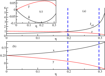
Although $\delta$ and $\gamma$ become nonzero for finite $\eta$ thus destroying the $SU(2)$ symmetry of the orbital sector, their values remain small in the physical regime for $\eta$ depicted in Fig. 10. It is therefore indeed reasonable to neglect this anisotropy in a first approximation as has been done in the previous section. Furthermore, we also find that $z\sim 1$ at least up to $\eta\sim 0.2$ so that the variation in $z$ can also be neglected. We are then back to Hamiltonian (2) with $J$ replaced by an effective superexchange scale $J_{\mathit{eff}}$ and with $x$ and $y$ being functions of the single parameter $\eta$ only. From this observation we can infer the basic properties of this model: For $\eta\lesssim 0.2$ the model will be in a “rescaled $SU(4)$ phase”, i.e., a phase where the same field theory as at the $SU(4)$ symmetric point describes the low-energy properties but with spin and orbital velocities which are rescaled and no longer equivalent. Strictly speaking this is only correct without orbital anisotropy ($\delta=\gamma=0$). Depending on the spin order, the orbital anisotropy might become Ising-like so that the orbital excitations become gapped. However, even if this happens the orbital gap caused by this mechanism will be extremely small. For $\eta\gtrsim 0.2$ we expect to enter a phase with ferromagnetically ordered spins and antiferromagnetic correlations in the orbital sector. At the same time $J_{\mathit{eff}}$ increases with increasing $\eta$ so that we expect a phase separated state if $\eta\gtrsim 0.3$ in the doped case.

In the following, we present numerical results for the full model (V) with $J/t=0.5$ and the parameters as given in Eqs. (V,13). In Fig. 11 the density as a function of chemical potential is shown for $\eta=0.3$ and $\eta=0.25$.

Figure 11: (color online) Density as a function of the chemical potential for $J/t=0.5$ and $\eta=0.3$. The inset shows the same for $\eta=0.25$. The lines are guides to the eye.

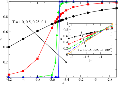
As in Fig. 6 we see that the density for $\eta=0.3$ and $T/t\to 0$ jumps from zero to one. Here the jump occurs at a chemical potential $\mu\approx-3.5$. Again this indicates a diverging compressibility in a canonical ensemble for all densities and confirms the expected phase separation at large $\eta$. For $\eta=0.25$ (shown the in the inset of Fig. 11), on the other hand, the ground state is not phase separated.

Next, we consider the slightly doped case, $n\sim 0.8-0.85$, for different parameters $\eta$. The nearest-neighbor correlation functions $\langle\boldsymbol{S}_{j}\boldsymbol{S}_{j+1}\rangle$ and $\langle\boldsymbol{\tau}_{j}\boldsymbol{\tau}_{j+1}\rangle$ presented in Fig. 12 show clearly that the spin correlations are antiferromagnetic for $\eta=0.1$ and ferromagnetic for $\eta=0.2$ and $\eta=0.25$.

Figure 12: (color online) TMRG results for model (V) with $J=0.5$ and $\eta=0.1,\,0.2,0.25$. The chemical potential is set to $\mu=0.6$ for $\eta=0.1$, $\mu=0.0$ for $\eta=0.2$, and $\mu=-0.8$ for $\eta=0.25$, respectively. (a) Nearest-neighbor spin-spin correlation $\langle\boldsymbol{S}_{j}\boldsymbol{S}_{j+1}\rangle$, (b) nearest-neighbor orbital-orbital correlation $\langle\boldsymbol{\tau}_{j}\boldsymbol{\tau}_{j+1}\rangle$, and (c) the density as a function of temperature. Note, that for the chemical potentials chosen here the densities depend only weakly on temperature, $n\sim 0.8-0.85$.

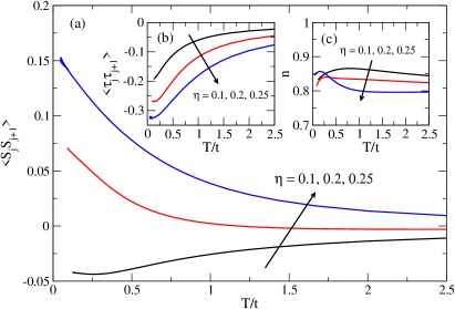
The orbital correlations, on the other hand, are antiferromagnetic in all three cases. To fix the critical value for $\eta$ where the phase transition occurs, we consider in Fig. 13 the nearest-neighbor spin correlation for the undoped model ($n=1$) as a function of temperature $T$ and Hund’s coupling $\eta$.

Figure 13: (color online) TMRG results for the nearest-neighbor correlation function $\langle\boldsymbol{S}_{j}\boldsymbol{S}_{j+1}\rangle$ in the undoped case for $J=0.5$ and different $\eta$. The red dashed curve denotes the result for $\eta=0.2$. The spins are fully polarized in the ground state, $\langle\boldsymbol{S}_{j}\boldsymbol{S}_{j+1}\rangle=1/4$ (black dot), if $\eta\gtrsim 0.2$.

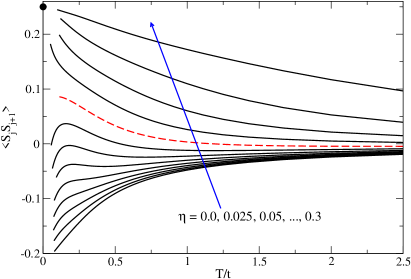
The data show that the spins in the ground state are fully polarized if $\eta>\eta_{c}\approx 0.2$. For $\eta<\eta_{c}$ the spin correlations are antiferromagnetic in the ground state. In this case, however, $\langle\boldsymbol{S}_{j}\boldsymbol{S}_{j+1}\rangle$ can be non-monotonic as a function of temperature and even larger than zero in a certain temperature range if $\eta$ is close to $\eta_{c}$. The expectation value for $\langle\boldsymbol{S}_{j}\boldsymbol{S}_{j+1}\rangle$ jumps at zero temperature from some $\eta$-dependent value for $\eta<\eta_{c}$ to $1/4$ for $\eta>\eta_{c}$. The phase transition driven by $\eta$ is therefore first order. Very interestingly, the phase transition occurs at a value for $\eta$ which is close to the one expected for LaTiO₃. In addition to the frustration of the orbital sector in this compound due to different orbital pairs being active along each direction, this closeness to the phase transition might also be important to understand the peculiar physics of LaTiO₃. It might, in particular, be a contributing factor to the smallness of the ordered moment in the G-type antiferromagnetic structure.Keimer et al. (2000) Note, however, that also other factors like the Ti-O-Ti bond angle are very important in determining whether the spins order ferro- or antiferromagnetically. The different magnetic properties of YTiO₃ (ferromagnetic spin order) and LaTiO₃ (G-type antiferromagnetic order), for example, have been ascribed to a small variation in this angle.Khaliullin and Okamoto (2003) Nevertheless, this variation in bond angle can be mimicked to a certain degree by increasing $\eta$ so that the phase transition situated at $\eta_{c}\approx 0.2$ in the one-dimensional model is indeed important to understand the physics of the cubic titanates.

Finally, we again want to study possible pairing instabilities in the slightly doped case. Here we concentrate on $\eta=0.25$ with $J=0.5$ and $\mu=-0.8$ as in Fig. 12. Results for the leading correlation lengths in this case are presented in Fig. 14.

Figure 14: (color online) Leading correlation lengths for $J=0.5$, $\eta=0.25$ and a chemical potential $\mu=-0.8$ corresponding to a density $n\sim 0.84$ at low temperatures (see Fig. 12(c)). The orbital-orbital and the density-density correlations show incommensurate oscillations at low temperatures as depicted in the inset whereas the spin-spin and the spin triplet/orbital singlet correlations are both non-oscillating.

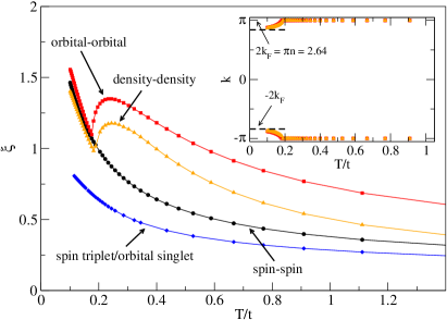
We find that the spin-spin, orbital-orbital, density-density, as well as the spin triplet/orbital singlet correlation lengths all diverge as $1/T$ for $T\to 0$ indicating that these correlations will decay algebraically at zero temperature. As in Sec. IV.2 we find that the oscillations of the orbital-orbital and the density-density correlation become incommensurate in the low temperature regime. Again $k\to\pm 2k_{F}=\pm\pi n\approx\pm 2.64$ for $n\sim 0.84$ reflecting the incommensurate filling of the system. The spin triplet/orbital singlet correlation length is larger than any of the other correlation lengths associated with the pair correlations defined in (III). If superconductivity can be stabilized at all in a possible nematic phase of LaTiO₃ or YTiO₃ there is therefore the possibility that it will be of triplet character.

VI Summary and Conclusions

In this paper we studied the thermodynamic properties of hole-doped one-dimensional Mott insulators with orbital degrees of freedom. We described such systems in terms of generalized (multi-band) $t-J$ models. Neglecting the Hund’s rule splitting of the virtually excited states we were led to a model which is integrable for one specific value of the ratio $J/t$. At this point the model becomes $SU(4|1)$ symmetric (graded $SU(5)$ symmetry) and belongs to the so called Uimin-Sutherland class of models.Sutherland (1975) The integrability at this particular point is analogous to the integrability of the usual $t-J$ model at the supersymmetric point. Ground-state properties of the $SU(4|1)$ symmetric spin-orbital model have been first investigated using Bethe ansatz by Schlottmann and Kawakami.Schlottmann (1992, 1993); Kawakami (1993) Here we presented a set of nonlinear integral equations also based on the Bethe ansatz which allowed us to study the thermodynamics. Using conformal field theory we have been able to connect our new results for the thermodynamics at low temperatures with the results for the ground state and the elementary excitations obtained by Schlottmann and Kawakami.

In the second part of the paper we used the density matrix renormalization group applied to transfer matrices (TMRG) to study the thermodynamics of the two-band $t-J$ model away from the integrable point. By comparing with Bethe ansatz results at the integrable point we first demonstrated that the obtained numerical results are accurate down to low temperatures $T/t\sim 0.05$. For large values of $J/t$ we then showed that the ground state becomes phase separated. Next, we studied the effects of hole doping on various phases of the undoped model. If the ground state of the undoped model is dimerized then the associated spin gap persists up to relatively large hole concentrations. The long-range nature of the dimer order, however, seems to break down immediately upon hole doping. Starting from the phase of the undoped model where the spins are fully ferromagnetically polarized and the orbitals show antiferromagnetic correlations we found that upon hole doping the spin triplet/orbital singlet pair correlation dominates among the various possible pair correlation functions. This correlation function will decay algebraically at zero temperature so that interchain couplings might stabilize true triplet superconductivity in this phase.

In the last part we used the TMRG algorithm to study the effects of hole doping for a one-dimensional version of a realistic model for cubic titanates. The model can be written in a form making it very similar to the one considered earlier. Previously independent parameters, however, now become functions of the ratio $\eta$ of Hund’s coupling $J_{H}$ and the onsite Coulomb repulsion $U$, and there is an additional $xxz$-type anisotropy of the orbital sector. The effective superexchange coupling is a function of $\eta$ as well and increases monotonically with increasing $\eta$. For $\eta\gtrsim 0.3$ this leads to a phase separated ground state. In addition, we find a phase transition at $\eta_{c}\approx 0.2$ between a state with antiferromagnetically correlated spins ($\eta<\eta_{c}$) and a state with fully ferromagnetically polarized spins ($\eta>\eta_{c}$). The phase transition is first order. For $\eta>\eta_{c}$ the dominating pair correlation is again of spin triplet/orbital singlet character and might lead to a true superconducting instability if interchain couplings are present. Interestingly, realistic $\eta$-values for LaTiO₃ are close to $\eta_{c}$. Although a purely one-dimensional model is not appropriate for this compound, the nature of local correlations might be correctly captured and $\eta$ being close to $\eta_{c}$ might contribute to the peculiar properties of this compound, in particular, to the extremely small G-type magnetic moment.

Appendix A Nonlinear integral equations

The integrable $SU(4|1)$ model admits the calculation of exact results for the thermodynamics. Here the largest eigenvalue of the QTM can be obtained by Bethe ansatz.Klümper et al. (1997) The number of Bethe ansatz equations, however, diverges in the limit $M\to\infty$. It is thus necessary to encode the Bethe ansatz equations into an alternative form for which the limit can be taken analytically. This can be done by defining suitable auxiliary functions in the spirit of Refs. Klümper, 1992, 1993, which are shown to be determined by a closed set of only finitely many coupled nonlinear integral equations (NLIEs).

The rigorous derivation depends on the explicit knowledge of the auxiliary functions in terms of the Bethe ansatz roots for finite $M$. Unfortunately these are unknown for the $SU(4|1)$ model. Yet we are able to conjecture the complete set of coupled NLIEs by generalizing the structure that has been found for two closely related models in the Uimin-Sutherland class, namely the $SU(2|1)$ and the $SU(4)$ models.Jüttner et al. (1997); Damerau and Klümper (2006) For the $SU(4|1)$ model we thus expect a total number of 15 coupled NLIEs, exactly one more than for the $SU(4)$ model. Their structure should be given by

$$\ln{b}^{({a})}_{j}(x)=-\frac{t{V}^{({a})}(x)+{c}^{({a})}_{j}}{T}\\ -\sum_{b=1}^{4}\sum_{k=1}^{\binom{4}{b}}\int_{-\infty}^{\infty}{K}^{({a,b})}_{j,k}(x-y)\ln{B}^{({b})}_{k}(y)\,\frac{\mathrm{d}y}{2\pi}$$ (14)

where ${B}^{({a})}_{j}(x)={b}^{({a})}_{j}(x)+1$ are the unknown auxiliary functions. The free energy is obtained from these functions via

$$f=-T\sum_{a=1}^{4}\sum_{j=1}^{\binom{4}{a}}\int_{-\infty}^{\infty}{V}^{({a})}(y)\ln{B}^{({a})}_{j}(y)\,\frac{\mathrm{d}y}{2\pi}\;.$$ (15)

Since the NLIEs must both reproduce the known results for the $SU(4)$ model in the limit $n\to 1$ ($\mu\to\infty$) and yield the correct zero-temperature limit, it is possible to fix the driving terms and kernel functions. We find

$${V}^{({a})}(x)=\frac{4a}{4x^{2}+a^{2}}$$ (16)

and the constants

$${c}^{({1})}_{1} ={c}^{({1})}_{2}=-2t-\mu-h/2$$

$${c}^{({1})}_{3} ={c}^{({1})}_{4}=-2t-\mu+h/2$$

$${c}^{({2})}_{1} =-4t-2\mu-h$$

$${c}^{({2})}_{2} ={c}^{({2})}_{3}={c}^{({2})}_{4}={c}^{({2})}_{5}=-4t-2\mu$$

$${c}^{({2})}_{6} =-4t-2\mu+h$$

$${c}^{({3})}_{1} ={c}^{({3})}_{2}=-6t-3\mu-h/2$$

$${c}^{({3})}_{3} ={c}^{({3})}_{4}=-6t-3\mu+h/2$$

$${c}^{({4})}_{1} =-8t-4\mu\;.$$ (17)

The kernel functions ${K}^{({a,b})}_{j,k}(x)$ for $a,b=1,2,3$ are similar to those of the $SU(4)$ model (see Ref. Damerau and Klümper, 2006 eqs. (33)–(35)), but where the common functions ${\widehat{K}}^{({a,b})}_{[4]}(k)$ are replaced by

$${\widehat{\mathcal{K}}}^{({a,b})}(k)=\text{e}^{(1-b)|k|/2}\,\frac{\sinh(ak/2)}{\sinh(k/2)}-\delta_{a,b}\;.$$ (18)

The remaining kernel functions are

$${K}^{({4,a})}_{1,j}(x)={K}^{({a,4})}_{j,1}(x)=\int_{-\infty}^{\infty}{\widehat{\mathcal{K}}}^{({a,4})}(k)\text{e}^{\text{i}kx}\,\mathrm{d}k\;.$$ (19)

The set of NLIEs can easily be solved numerically by iteration yielding high accuracy over the whole parameter range. The validity of the results has been checked by comparing our specific heat data to the high-temperature expansion rigorously derived in Ref. Tsuboi, 2006 on the basis of an alternative set of NLIEs. Moreover, the results agree in the low-temperature limit with CFT and over the whole temperature range with numerical TMRG calculations as shown in this article.

References

- Tokura and Nagaosa (2000) Y. Tokura and N. Nagaosa, Science 288, 462 (2000).
- Khaliullin (2005) G. Khaliullin, Prog. of Theo. Phys. Suppl. 160, 155 (2005).
- Lee et al. (2006) S. Lee, J.-G. Park, D. T. Adroja, D. Khomskii, S. Streltsov, K. A. McEwen, H. Sakai, K. Yoshimura, V. I. Anisimov, D. Mori, et al., Nature Mat. 5, 471 (2006).
- Khomskii and Mizokawa (2005) D. I. Khomskii and T. Mizokawa, Phys. Rev. Lett. 94, 156402 (2005).
- Ulrich et al. (2003) C. Ulrich, G. Khaliullin, J. Sirker, M. Reehuis, M. Ohl, S. Miyasaka, Y. Tokura, and B. Keimer, Phys. Rev. Lett. 91, 257202 (2003).
- Sirker and Khaliullin (2003) J. Sirker and G. Khaliullin, Phys. Rev. B 67, 100408(R) (2003).
- Li et al. (1998) Y. Q. Li, M. Ma, D. N. Shi, and F. C. Zhang, Phys. Rev. Lett. 81, 3527 (1998).
- Yamashita et al. (1998) Y. Yamashita, N. Shibata, and K. Ueda, Phys. Rev. B 58, 9114 (1998).
- Pati and Singh (2000) S. K. Pati and R. R. P. Singh, Phys. Rev. B 61, 5868 (2000).
- Frischmuth et al. (1999) B. Frischmuth, F. Mila, and M. Troyer, Phys. Rev. Lett. 82, 835 (1999).
- Itoi et al. (2000) C. Itoi, S. Qin, and I. Affleck, Phys. Rev. B 61, 6747 (2000).
- Azaria et al. (2000) P. Azaria, E. Boulat, and P. Lecheminant, Phys. Rev. B 61, 12112 (2000).
- Pati et al. (1998) S. K. Pati, R. R. P. Singh, and D. I. Khomskii, Phys. Rev. Lett. 81, 5406 (1998).
- Sirker (2004) J. Sirker, Phys. Rev. B 69, 104428 (2004).
- Chen et al. (2007) Y. Chen, Z. D. Wang, Y. Q. Li, and F. C. Zhang, Phys. Rev. B 75, 195113 (2007).
- Sutherland (1975) B. Sutherland, Phys. Rev. B 12, 3795 (1975).
- Schlottmann (1992) P. Schlottmann, Phys. Rev. Lett. 69, 2396 (1992).
- Schlottmann (1993) P. Schlottmann, J. Phys.: Cond. Mat. 5, 313 (1993).
- Kawakami (1993) N. Kawakami, Phys. Rev. B 47, 2928(R) (1993).
- Affleck (1986) I. Affleck, Nucl. Phys. B 265, 409 (1986).
- Frahm and Schadschneider (1993) H. Frahm and A. Schadschneider, J. Phys. A: Math. Gen. 26, 1463 (1993).
- Izergin et al. (1989) A. G. Izergin, V. E. Korepin, and N. Y. Reshetikhin, J. Phys. A: Math. Gen. 22, 2615 (1989).
- Ogata et al. (1991) M. Ogata, M. U. Luchini, S. Sorella, and F. F. Assaad, Phys. Rev. Lett. 66, 2388 (1991).
- Hellberg and Mele (1991) C. S. Hellberg and E. J. Mele, Phys. Rev. Lett. 67, 2080 (1991).
- Kawakami and Yang (1991) N. Kawakami and S.-K. Yang, Phys. Rev. B 44, 7844 (1991).
- I.Peschel et al. (1999) I.Peschel, X. Wang, M. Kaulke, and K. Hallberg, eds., Density-Matrix Renormalization, Lecture Notes in Physics, vol. 528 (Springer, Berlin, 1999), and references therein.
- Glocke et al. (2008) S. Glocke, A. Klümper, and J. Sirker, in Computational Many-Particle Physics (Springer, Berlin, 2008), vol. 739 of Lecture Notes in Physics.
- Sirker and Klümper (2002a) J. Sirker and A. Klümper, Europhys. Lett. 60, 262 (2002a).
- Klümper et al. (1999) A. Klümper, R. Raupach, and F. Schönfeld, Phys. Rev. B 59, 3612 (1999).
- Mutou et al. (1998) T. Mutou, N. Shibata, and K. Ueda, Phys. Rev. Lett. 81, 4939 (1998).
- Sirker and Klümper (2002b) J. Sirker and A. Klümper, Phys. Rev. B 66, 245102 (2002b).
- Ammon et al. (1999) B. Ammon, M. Troyer, T. M. Rice, and N. Shibata, Phys. Rev. Lett. 82, 3855 (1999).
- Glocke et al. (2007) S. Glocke, A. Klümper, and J. Sirker, Phys. Rev. B 76, 155121 (2007).
- Sirker et al. (2008) J. Sirker, A. Herzog, A. M. Oleś, and P. Horsch, arXiv:0807.4693 (2008).
- Takahashi (1986) M. Takahashi, Prog. Theor. Phys. Supp. 87, 233 (1986).
- Klümper et al. (2001) A. Klümper, J. R. R. Martinez, C. Scheeren, and M. Shiroishi, J. Stat. Phys. 102, 937 (2001).
- Khaliullin and Maekawa (2000) G. Khaliullin and S. Maekawa, Phys. Rev. Lett. 85, 3950 (2000).
- Keimer et al. (2000) B. Keimer, D. Casa, A. Ivanov, J. W. Lynn, M. v. Zimmermann, J. P. Hill, D. Gibbs, Y. Taguchi, and Y. Tokura, Phys. Rev. Lett. 85, 3946 (2000).
- Khaliullin and Okamoto (2003) G. Khaliullin and S. Okamoto, Phys. Rev. B 68, 205109 (2003).
- Klümper et al. (1997) A. Klümper, T. Wehner, and J. Zittartz, J. Phys. A 30, 1897 (1997).
- Klümper (1992) A. Klümper, Ann. Phys. 1, 540 (1992).
- Klümper (1993) A. Klümper, Z. Phys. B 91, 507 (1993).
- Jüttner et al. (1997) G. Jüttner, A. Klümper, and J. Suzuki, Nucl. Phys. B 487, 650 (1997).
- Damerau and Klümper (2006) J. Damerau and A. Klümper, J. Stat. Mech. 0612, P014 (2006).
- Tsuboi (2006) Z. Tsuboi, Nucl. Phys. B 737, 261 (2006).