Network effects in a human capital based economic growth model
Abstract
We revisit a recently introduced agent model [ACS 11, 99 (2008)], where economic growth is a consequence of education (human capital formation) and innovation, and investigate the influence of the agents’ social network, both on an agent’s decision to pursue education and on the output of new ideas. Regular and random networks are considered. The results are compared with the predictions of a mean field (representative agent) model.
keywords:
Econophysics , agent based models , human capital , complex networksPACS:
89.75-k , 89.65.Gh , 89.75.Hc , 87.23.Ge,
,
and
1 Introduction
Recent theoretical macroeconomic growth models emphasize the ultimate sources of growth. In these so called ’endogenous growth models’, the long-run rate of growth depends on a set of parameters that describe some inner characteristics of the economy. These characteristics may be connected to preferences (e. g. the relative importance of future consumption), to some technological restrictions (e. g. the shape of the aggregate production function), to demographic factors, to the degree of economic openness, to the quality of institutions, and, last but not least, to the ability of producing and adopting innovation, usually related to education and research and development activities.
An important fraction of agent-based models in the economics literature concerns innovation and diffusion processes ([1] – [5]). Some of these relate to economic growth in an evolutionary economics perspective, as in the seminal work of Nelson and Winter [6]. The latter emphasized some of the neoclassical theory drawbacks concerning the modeling consistency between microeconomic technical change and macroeconomic approaches to growth. The evolutionary approach seeks then a successful combination of the micro and aggregate pictures, usually resorting to computer simulation modeling approaches. In what concerns economic growth models, Araújo and St. Aubyn’s [7] approach, which we develop here, innovates within the evolutionary economics based endogenous growth literature. They were pioneer in relying on ideas-based macroeconomic growth and on the education decision and outcome interactions and dynamics among agents, and not so much on the more usually described local innovation processes that swell through the economy. In their endogenous growth model ’ideas’ or ’inventions’ are the main growth engine. These ideas are non-rival, in the sense that they can be used by some without diminishing the possibility of its use by others. Examples relevant to economic growth are easy to find – the power engine, electricity, or the computer come almost immediately to mind. Ideas are produced by skilled labor, as proposed by Jones [8]. Araújo and St. Aubyn’s model, however, departs from more conventional approaches in what concerns the way the skilled fraction of the labor force is determined. In their agent-based approach, individuals are subject to interaction or neighborhood effects, and the decision to become educated depends not only on an economic reasoning, but also on a degree of social conditioning. As it will become clear later, the skilled or educated share of the population is a key factor in what concerns the economy’s rate of growth.
Networks of interacting agents play an important modeling role in fields as diverse as computer science, biology, ecology, economy and sociology. An important notion in these networks is the distance between two agents. Depending on the circumstances, distance may be measured by the strength of interaction between the agents, by their spatial distance or by some other norm expressing the existence of a link between the agents. Based on this notion, global parameters have been constructed to characterize the connectivity structure of the networks. Two of them are the clustering coefficient (CC) and the characteristic path length (CPL) or geodesic distance. The clustering coefficient measures the average probability that two agents, having a common neighbor, are themselves connected. The characteristic path length is the average length of the shortest path connecting each pair of agents. These coefficients are sufficient to distinguish randomly connected networks from ordered networks and from small-world networks. In ordered networks, the agents being connected as in a crystal lattice, clustering is high and the characteristic path length is large too. In randomly connected networks, clustering and path length are low, whereas in small-world networks [9], [10] clustering may be high while the path length is kept at a low level. Starting from a regular structure and applying a random rewiring procedure (to interpolate between regular and random networks) it has been found [9] that there is a broad interval of structures over which CPL is almost as small as in random graphs and yet CC is much greater than expected in the random case and a small-world network is obtained. An alternative way to generate a small-world network is by adding a small number of random short-cuts to a regular lattice.
A small characteristic path length and very high clustering are found in real social networks, together with a non-uniform distribution of node connectivities. Other distinctive features of this type of networks are positive degree correlations (assortative mixing) and the existence of a community structure [11], [12].
In the present paper, we investigate the role of the network of interactions in the model introduced by Araújo and St Aubyn [7]. The aim is to clarify to what extent the conclusions of [7] depend on the simplified topology of agents interactions assumed in that work. We have simulated the model on networks with some of the features described above, namely on regular square lattices, classical random (Erdős-Rényi) graphs as well as small-world networks. An analytical study of the model, using a mean-field-like approximation, is also presented.
The original model definitions and results are reviewed in the next section. In section 3 we present the mean field results. Simulations on random networks are detailed in section 4, and section 5 is devoted to a discussion of the results. Conclusions are presented in the final section.
2 Araújo and St Aubyn’s model
In the model economy introduced in [7] there is a constant population of individuals (agents), who live for two periods of time; each individual is a junior in the first period and becomes a senior in the second period of his life. There is generations overlap and one further assumes that at any time there are juniors and seniors. Agents are either skilled or unskilled; an unskilled junior is part of the unskilled labor force, whereas a skilled junior is a student who postpones joining the (skilled) labor force until he becomes a (skilled) senior. Unskilled juniors will later turn to unskilled seniors.
Denoting respectively by , , and the total number of skilled juniors, unskilled juniors, skilled seniors and unskilled seniors, one has
| (1) | |||||
| (2) | |||||
| (3) |
and the total number of unskilled workers is
| (4) |
Individuals live at fixed positions in space – which is taken in [7] as a one-dimensional regular lattice with periodic boundary conditions.
One may then represent the state of agent () by a ’microscopic’ variable which takes one out of four values; (skilled junior), (unskilled junior), (skilled senior) and (unskilled senior).
At fixed time intervals (periods) the states of all agents are updated simultaneously, according to deterministic rules. Agents in junior states turn into the corresponding senior state (, ); an agent in a senior state is replaced by either a skilled or an unskilled junior, depending on the result of a ’decision rule’. The decision of a junior agent to follow education is determined both by imitation of his neighbors (neighborhood effect) and by external information (concerning the relative wages of skilled and unskilled workers). According to model [7], a ’newborn’ agent will become a student if there is a weighted majority of skilled agents in his neighborhood. More precisely if
| (5) |
where () is the number of senior skilled (unskilled) neighbors of agent and is the relative weight of the skilled, given by
| (6) |
In (6) () denotes the skilled (unskilled) workers’ salary and is an external parameter, accounting for a bias towards education and corrections due to discount rate [13]. A larger value of may represent a positive bias towards education and/or that the future is less valued. If condition (5) is not fulfilled, agent becomes an unskilled junior ().
Production
Skilled (intellectual) and unskilled (manual) workers have distinct roles in the model economy: intellectual workers produce ideas whereas manual workers use existing ideas to produce final goods. Denoting by the present stock of ideas, the final production function is written as
| (7) |
New ideas are created according to
| (8) |
with
denoting the distance between skilled seniors and . When , the second term in (8) yields a reinforcement of the output of ideas if skilled workers are close to each other – is hence called the team effect parameter. Parameter is related to skilled labor marginal productivity.
The total income is distributed as wages and split between unskilled and skilled labor forces, . The share of each class of workers is assumed to be the result of a social pact [14] and is given by
| (9) | |||
| (10) |
yielding individual salaries
| (11) | |||
| (12) |
The current value of the relative wage is taken into account whenever a new agent makes his choice regarding education (eq. 5). Notice that, in the absence of team effect (),
| (13) |
– thus the existence of a large number of unskilled workers is a stimulus to education.
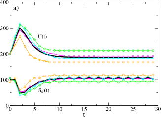
It is easily seen from eqs. (7) - (12) that the dynamics described above has two trivial absorbing states: and . The former case implies a collapse of the economy () due to over-education – no manual workers exist – and may be avoided by a modification of eqs (9) and (10) [7]. The outcome is less severe when , in which case one gets a stagnation of the economy (), a situation referred to as the poverty trap. The system’s asymptotic state depends on parameter values and also on the initial configuration of agents. When it does not collapse to an absorbing state, a finite system may reach a nontrivial fixed point, with a constant number of skilled and unskilled workers; more often, the asymptotic state is characterized by a stationary number of unskilled workers, while the number of skilled ones oscillates between two values – see Figure 1 (a). This is a consequence of the somewhat artificial junior to senior updating rule [15]. Still, one may argue that the appropriate time unit is a generation (equal to two periods) and consider a state where observables are constant along generations a ’steady state’.
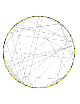
In [7] an initial state is generated, with a pre-assigned ratio of skilled to unskilled workers, randomly placed on a ring of size . Fixing the size of the neighborhood (eq. 4) and the values of the exogenous parameters, a baseline and several scenarios were considered. In each case, equations (5) - (12) were iterated till a ’stationary state’ was reached, and the process was repeated for other realizations of the initial state. A segregation of educated and uneducated agents in separate domains was observed, specially when team effects were taken into account – see Figure 2. The team effect also yielded higher economic growth and qualification, usually together with lower relative salary levels for skilled workers. The steady state was found to depend on the initial number of intellectual workers, a poor concentration of educated agents leading to lower growth rates and lower percentage of skilled workers.
3 Mean field (representative agent) approach
In the model described above, the evolution of the economy is directly determined by the overall numbers of skilled and unskilled workers (and by their relative positions if the team effect is considered). The random initial position of the four types of agents is the sole source of stochasticity in the model, since for a particular distribution of agents in space, the decision (to study or not to study) is predictable.
In mean field approximations, one neglects fluctuations of the microscopic variables and replaces the detailed form of their mutual interactions by the interaction of a single microscopic variable with a uniform ’mean field’, which depends on the state of the system. In the present case, neglecting the differences in the local neighborhood would lead to one of the two trivial outcomes, ’all educated’ or ’all uneducated’. One can, however, obtain a related non trivial model, within the mean field spirit, by considering a single representative agent who takes the decision of whether or not to follow education stochastically, with relative probabilities depending on the total number of skilled to unskilled workers at that time. In this mean field model (MF) one has uniform initial conditions (or neighborhood) and probabilistic decision making, instead of the random initial conditions and deterministic decision of the original model. More specifically, we set
| (14) |
where is the probability that a junior decides to study, and assume the decision probabilities depend on the weighted ratio of skilled to unskilled seniors
| (15) |
(; is the relative weight given to the skilled, as before). Substituting eq. (15) into eq. (14) one obtains a deterministic nonlinear equation [16] with a stable nontrivial solution, as shown below.
A recursion relation is easily written for :
| (16) |
where is the product of the education bias by the efficency of skilled workers (). Provided , this equation has stationary solutions or
| (17) |
independent of initial conditions. From equations (14) - (17) one easily gets the
following (MF) stationary values:
relative wages
| (18) |
number of unskilled workers
| (19) |
number of skilled workers
| (20) |
growth rate
| (21) |
The requirement puts a limit on parameter values: . The fact that the stationary number of unskilled workers is independent of (eq. (19)) is obviously a spurious result of the mean field approximation! The prediction for the other observables is, however, not far from the simulation results for a regular lattice – see Table 2 – suggesting that, in the absence of team effect, the model introduced in [7] is well approximated by the mean field model, exception made of the steady state growth rate dependency on initial values.
4 Simulations on complex networks
The ring topology used in [7] is obviously a simplified description of the structure of the social interactions between agents. The mean field approach, on the other hand, assumes that the underlying network is a complete graph where each individual is influenced by all the others – which is only a good approximation for well-mixed populations. In this section we present the results of model simulations on more realistic social networks.
As described in section 2, agents live on the nodes of a network, which we call the influence network, since a ’newborn’ agent is influenced by his neighborhood on this network, in his decision concerning education. When team effects are considered (see eq. (8)), the output of ideas is enhanced if the ’distance’ between pairs of skilled workers is small. This distance may be the euclidean one on a regular lattice or the shortest path along links of a random network. One may even consider a collaboration network among senior skilled agents, distinct from the underlying influence network. Take for example a situation where education is decided on a family/local neighbors basis, whereas intellectual workers collaborate with colleagues from a distant town by e-mailing or indirectly through mutual acquaintances. This case can be modeled by taking a square lattice (with a neighborhood of size or ) as influence network, plus a small-world for the collaboration network.
Regular lattices
A comparison was made between the results for a ring and a square lattice with periodic
boundary conditions and the same number of neighbors ( or ).
Random networks
-
•
classical random graph (CRG)
In each run, a connected graph was generated with vertices and edges through a random graph process: a randomly chosen pair of vertices is linked by an edge and the process is repeated till the pre-defined number of edges, , is obtained (disregarding graphs with self-loops or multiple edges). -
•
small-world networks (SW)
Taking a ring or a square lattice as ’mother lattice’, short-cuts between randomly chosen nodes were added with (small) probability per regular link of the underlying lattice ( short-cuts). We have considered the following cases: i) only the influence network is SW (the additional random links are only relevant for the education decision), ii) only the collaboration network is a SW (only senior skilled agents may get additional random links) and iii) both networks are SW. The addition of random links is repeated every half generation, so a senior agent keeps the regular contacts he had while a junior but is free to establish new short-cuts, and a newborn junior does not inherit random links.
In our simulations we have used agents and chosen parameter values which yield reasonable stationary growth rates (we verified that a change in parameter values does not produce qualitatively distinct conclusions). A calibration was done using mean-field equations (17) - (21), assuming a annual growth rate with a half generation of years (or ) and fixing . One obtains the baseline parameter values: , (), . To study team effects (scenario 5 in [7]) we took .
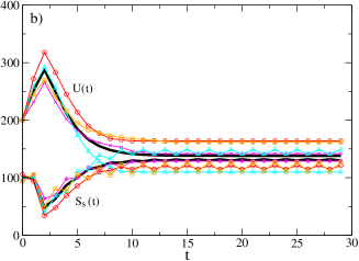
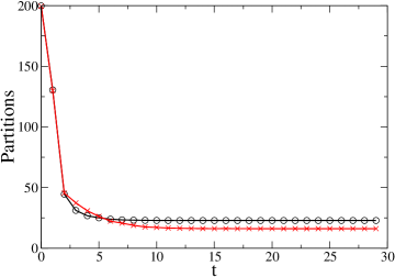
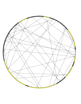
Simulations started with unskilled workers randomly placed on the network nodes. Averages over up to samples were taken for each set of parameters (neglecting samples which collapsed to an absorbing state). Typical evolutions of the populations of skilled and unskilled workers in single runs are represented in Figure 1, together with the respective average over runs, for the case of (a) a ring and (b) a small-world network (case ii), with team effect parameters. The period-two oscillatory behaviour of the number of skilled seniors, discussed in section 2, yiels synchronous oscillations of the product growth rate, but with rather small amplitude (roughly equal to times the skilled workers’ amplitude). An illustration of an initial and final network configurations, where domain formation is evident, is presented in Figure 3, for the case of a small-world built upon a ring. For the parameter values used in the simulations, relaxation times varied from about to periods (the relaxation is slower when the influence network is a small-world with few short-cuts). The overall picture is, however, qualitatively similar for all types of networks, with or without team effect. Simulation results for the ’steady state’ values of observables are summarized in Tables and .
5 Discussion
Our simulations confirm the statement [7] that, within this model, in the long run, higher growth rates are associated with higher qualification (more skilled workers and less unskilled ones) and stronger segregation by educational level. Usually this also implies smaller (relative) salaries for the intellectual workers.
From Tables 1 and 2, one sees that baseline results are rather similar for a ring or a square lattice with the same number of neighbors and they also do not differ significantly for a random graph with the same average degree. In contrast, a clear increase in qualification is obtained if the influence network is a small-world (specially for higher values) [17].
When team effects are taken into account, the effect of random inter-agent connections is evident from the much higher growth rates and larger fraction of skilled workers. Since collaboration networks are often found to be scale-free [18], we also ran simulations where the number of links between senior intellectuals had a power-law distribution (with exponent ). Those were not true scale-free networks, since the number of nodes was just about , but the purpose was to check if significant changes were seen. The results were very similar to the SW-case iii) with , except for a larger growth rate (). In the case of regular lattices, team effects are much stronger in 2d than in 1d (due to the higher clustering of the square lattice), yielding increased growth/qualification in two dimensions. The tendency for segregation is stronger on the (more realistic) 2d substract, as shown by the smaller number of partitions (domains) - see Table 2.
We have run simulations for higher numbers of agents and obtained qualitatively the same behavior, but the fraction of skilled workers increases with , leading to higher growth rates. Theoretical endogenous growth models often display this type of behavior, with larger economies tending to have higher growth rates [19]. Still, is too small for most realistic economies, so the values presented in Tables and should be taken just as indicative for the sake of comparison, and not on absolute terms.
6 Conclusion
In this work we have studied a simple agent model [7] designed to explain how economic growth can be the result of innovation introduced by a fraction of the population with higher education. The original unidimensional model was generalized by assuming that agents interactions took place on a more realistic type of social network.
The effect of assuming a heterogeneous interaction network may be summarized, in broad terms, as leading to a steady state with higher growth and qualification and a stronger segregation of skilled and unskilled individuals. As expected, this is specially notorious when team effects are considered, due to the shorter average distance between agents.
We have also derived and solved a related mean field model, which is able to reproduce some important results of the original model (without team effect). Note, however, that the mean field approximation leaves out the steady state growth rate dependency on initial values. Also, by assuming heterogeneous agents, one is able to reproduce cluster formation and to take into account a team contribution.
It will be interesting to consider a more microscopic version of the model, with heterogeneous salaries depending on the agent’s productivity (as well as on overall economic state). The artificial decision rule (5), may be replaced by the agent making his choice according to the sign of a local field, as usually done in models of social influence with binary decision [20]. The question is then how to relate agent variables to production and innovation in an economically sensible way.
Acknowledgment
T. A. and M. S. acknowledge support from FCT (Portugal),
Project PDCT/EGE/60193/2004. T.V.M. is supported by FCT (Portugal) through
Grant No.SFRH/BD/23709/2005.
UECE and Centro de Física do Porto are
supported by FCT (Fundação para a Ciência e a Tecnologia, Portugal),
financed by ERDF and Portuguese funds.
References
- [1] Chiaromonte F. and G. Dosi, Heterogeneity, Competition, and Macroeconomic Dynamics, Structural Change and Economic Dynamics 4, 39 (1993).
- [2] Dosi G., L. Marengo and G. Fagiolo, Learning in Evolutionary Environments, in Evolutionary Foundations of Economics, ed. K. Dopfer (Cambridge University Press, Cambridge, 2005).
- [3] Fagiolo, G. and G. Dosi, Exploitation, Exploration and Innovation in a Model of Endogenous Growth with Locally Interacting Agents, Structural Change and Economic Dynamics, 14, 237 (2003).
- [4] Silverberg, G. and B. Verspagen, Learning, Innovation and Economic Growth: A Long-Run Model of Industrial Dynamics, Industrial and Corporate Change, 3, 199 (1994).
- [5] Silverberg, G. and B. Verspagen Collective Learning, Innovation and Growth in a Boundedly Rational, Evolutionary World, Journal of Evolutionary Economics, 4, 207 (1994).
- [6] Nelson R. R. and Winter S.G., An Evolutionary Theory of Economic Change, (Harvard University Press, 1982).
- [7] T. Araújo and M. St. Aubyn, Education, Neighbourhood Effects and Growth: An Agent Based Approach, ACS - Advances in Complex Systems, 11, 99 (2008).
- [8] C. Jones, Growth and Ideas, in Handbook of Economic Growth, vol. 1B, eds. P. Aghion and S. Durlauf (Elsevier Science, Amsterdam, 2005).
- [9] D. J. Watts and S. H. Strogatz; Collective dynamics of small-world networks, Nature 393, 440 (1998).
- [10] D. J. Watts, Small Worlds (Princeton University Press, Princeton, 1999).
- [11] M. E. J. Newman and J. Park, Why social networks are different from other types of networks, Phys. Rev. E 68, 036122 (2003)
- [12] Parongama Sen, Complexities of social networks: A Physicist’s perspective, in Econophysics and Sociophysics: Trends and perspectives, ed. B. K. Chakrabarti, A. Chakrabarti and A. Chatterjee, Wiley-VCH (2006); e-print arXiv:physics/0605072
- [13] In the notation of [7] where is an increasing function of the discount rate .
- [14] The social pact ensures that unskilled workers earn what would have been produced if there were no skilled workers in society, and that skilled workers get the extra income derived from new ideas.
- [15] The number of skilled juniors takes the same asymptotic values, shifted in time by one period (conditions (2) and (3)).
- [16] We thank one of the referees for this clarifying comment.
- [17] Note that the SW built by adding shortcuts to a regular lattice with neighbors, has slightly higher average degree .
- [18] M. Newman, The structure of scientific collaboration networks, PNAC 98, 404 (2001)
- [19] C. Jones, Growth: With or Without Scale Effects?, American Economic Review, American Economic Association, 89, 139 (1999).
- [20] See e.g. Q Michard and J.-P. Bouchaud, Theory of collective opinion shifts: from smooth trends to abrupt swings, Eur. Phys. J. B 47, 151 (2005)
| Ring | SW - Decision | SW - Team Effect | SW - Dec.+ Team | CRG | MF | ||||||||
|---|---|---|---|---|---|---|---|---|---|---|---|---|---|
| Base | Team | p=0.03 | p=0.1 | p=0.03 | p=0.1 | p=0.03 | p=0.1 | Base | Team | Base | |||
| Base | Team | Base | Team | ||||||||||
| 0.666 | 1.79 | 1.06 | 2.23 | 1.09 | 2.25 | 2.78 | 3.33 | 3.16 | 3.78 | 0.67 | 3.67 | 1.09 | |
| 3.05 | 3.20 | 2.26 | 2.24 | 2.22 | 2.21 | 3.11 | 3.09 | 2.20 | 2.17 | 3.05 | 3.11 | 2.22 | |
| 60.6 | 104.9 | 96.8 | 132.9 | 99.1 | 133.1 | 128.9 | 136.1 | 148.3 | 155.1 | 61.1 | 140.2 | 100 | |
| 277.5 | 187.3 | 205.5 | 133.6 | 202.1 | 134.9 | 141.0 | 126.3 | 102.4 | 89.3 | 277.4 | 119.1 | 200 | |
| Partitions | 23.1 | 16.4 | 14.7 | 12.4 | 16.7 | 15.2 | 14.3 | 13.3 | 11.1 | 12.1 | 22.1 | 12.7 | - |
| Team Eff | - | 0.635 | - | 0.770 | - | 0.765 | 1.36 | 1.83 | 1.56 | 2.06 | - | 2.12 | - |
| Ring | Ring/SW -Team Effect | Square | Square/SW -Team Effect | MF | |||||
| Base | Team | p=0.03 | p=0.1 | Base | Team | p=0.03 | p=0.1 | Base | |
| 0.760 | 1.25 | 2.04 | 2.61 | 0.762 | 1.92 | 2.37 | 2.75 | 1.09 | |
| 2.79 | 3.35 | 3.30 | 3.28 | 2.82 | 3.24 | 3.01 | 2.97 | 2.22 | |
| 69.1 | 81.1 | 108.6 | 120.5 | 69.3 | 107.4 | 120.7 | 128.2 | 100 | |
| 253.6 | 230.6 | 175.7 | 151.1 | 256.2 | 180.9 | 153.1 | 138.2 | 200 | |
| Partitions | 35.0 | 31.9 | 25.9 | 24.3 | 9.3 | 6.7 | 7.4 | 7.9 | - |
| Team Eff | - | 0.357 | 0.845 | 1.29 | - | 0.742 | 1.04 | 1.34 | - |