Effective convergence of the 2PI-$1/N$ expansion for nonequilibrium quantum fields

Abstract

The $1/N$ expansion of the two-particle irreducible effective action offers a powerful approach to study quantum field dynamics far from equilibrium. We investigate the effective convergence of the $1/N$ expansion in the $O(N)$ model by comparing results obtained numerically in $1+1$ dimensions at leading, next-to-leading and next-to-next-to-leading order in $1/N$ as well as in the weak coupling limit. A comparison in classical statistical field theory, where exact numerical results are available, is made as well. We focus on early-time dynamics and quasi-particle properties far from equilibrium and observe rapid effective convergence already for moderate values of $1/N$ or the coupling.

Introduction – The need to understand the dynamics in heavy ion physics and the quark gluon plasma as well as highly nonlinear phenomena in the (post-)inflationary universe has lead to substantial development in the study of quantum field evolution far from equilibrium. One particular approach, firmly based on functional methods in field theory, employs the two-particle irreducible (2PI) effective action Berges:2004yj . The nonperturbative 2PI-$1/N$ expansion Berges:2001fi ; Aarts:2002dj , where $N$ denotes the number of matter field components, has in particular proven fruitful. In recent years this approach has been applied to a variety of nonequilibrium problems in $3+1$ dimensions, related to inflationary preheating Berges:2002cz ; Arrizabalaga:2004iw , effective prethermalization Berges:2004ce , fermion dynamics Berges:2002wr , transport coefficients Aarts:2003bk and kinetic theory Juchem:2004cs ; Berges:2005md , slow-roll dynamics Aarts:2007qu , topological defects Rajantie:2006gy , nonthermal fixed points Berges:2008wm , expanding backgrounds Tranberg:2008ae , nonrelativistic cold atoms Gasenzer:2005ze , etc. Besides these applications, theoretical aspects are under continuous investigation: renormalization in equilibrium is by now well understood vanHees:2001ik ; Blaizot:2003br ; Berges:2004hn and practical implementations of renormalization out of equilibrium are being developed Borsanyi:2008ar . Moreover, progress in adapting these methods to gauge theories is steady Arrizabalaga:2002hn ; Reinosa:2006cm ; Borsanyi:2007bf .

Applications of 2PI effective action techniques are based on truncations, employing either a weak coupling or a large $N$ expansion. So far, truncations stop at relatively low order: as far as we are aware all studies in field theory use next-to-leading order (NLO) truncations in the coupling or $1/N$ . The reason for this situation is clear: beyond NLO the complexity of the equations and the numerical effort required to solve them increases dramatically Aarts:2006cv . In this paper we present the first results beyond NLO in field theory.

Remarkably, the lowest order truncations beyond mean field theory include already many of the physical processes necessary to describe quantum field dynamics both far and close to equilibrium and are capable of capturing effective memory loss, universality of late time evolution, and thermalization. The natural question to ask is then how accurate a truncation at a given order describes the dynamics in the full theory. There are several ways this can be investigated. In the case of a systematic expansion, it should be possible to compare different orders of the expansion, shedding light on the effective convergence. When restricting to LO and NLO truncations only, the applicability of this approach is limited. The reason is that in LO mean field approximations scattering is absent and there is no notion of equilibration and thermalization, as there is at NLO. It is therefore necessary to consider the next-to-next-to-leading order (N²LO) contribution as well. In the first part of this paper we study this problem in the $O(N)$ model and compare the dynamics obtained at LO, NLO and (part of) N²LO in the $1/N$ expansion in quantum field theory. In cases where an exact solution is available, a direct comparison can be carried out, and this approach has been successfully applied using classical statistical field theory instead of quantum field theory Aarts:2000wi ; Aarts:2001yn . In the classical limit, the nonperturbative solution can be constructed numerically by direct integration of the field equations of motion, sampling initial conditions from a given probability distribution. We use this approach to further quantify the role of truncations in the second part of the paper.

2PI dynamics – We consider a real $N$-component scalar quantum field with a $\lambda(\phi_{a}\phi_{a})^{2}/(4!N)$ interaction ($a=1,\ldots,N$). In order to allow for an economical $1/N$ expansion, an auxiliary field $\chi$ is introduced to split the four-point interaction, which results in the action

$$S[\phi,\chi]=-\int_{\cal C}dx^{0}\int d{\mathbf{x}}\,\Big{[}\frac{1}{2}\partial_{\mu}\phi_{a}\partial^{\mu}\phi_{a}+\frac{1}{2}m^{2}\phi_{a}\phi_{a}$$

$$-\frac{3N}{2\lambda}\chi^{2}+\frac{1}{2}\chi\phi_{a}\phi_{a}\Big{]}.$$ (1)

The theory is formulated along the Schwinger-Keldysh contour ${\cal C}$, as is appropriate for initial value problems. In the symmetric phase ($\langle\phi_{a}\rangle=0$), the 2PI effective action depends on the one-point function $\bar{\chi}=\langle\chi\rangle$ and the two-point functions

$$G_{ab}(x,y) = G(x,y)\delta_{ab}=\langle T_{\cal C}\phi_{a}(x)\phi_{b}(y)\rangle,$$ (2)

$$D(x,y) = \langle T_{\cal C}\chi(x)\chi(y)\rangle-\langle\chi(x)\rangle\langle\chi(y)\rangle.$$ (3)

In terms of those, the action is parametrized as Cornwall:1974vz ; Aarts:2002dj

$$\!\!\!\!\!\Gamma[G,D,\bar{\chi}]=S[0,\bar{\chi}]+\frac{i}{2}\hbox{Tr}\ln G^{-1}+\frac{i}{2}\hbox{Tr}\,G_{0}^{-1}\left(G-G_{0}\right)$$

$$\;\;\;\;+\frac{i}{2}\hbox{Tr}\ln D^{-1}+\frac{i}{2}\hbox{Tr}\,D_{0}^{-1}\left(D-D_{0}\right)+\Gamma_{2}[G,D],$$ (4)

where $G_{0}^{-1}=i(\square+m^{2}+\bar{\chi})$ and $D_{0}^{-1}=3N/(i\lambda)$ denote the free inverse propagators. Extremizing the effective action gives equations for $\bar{\chi}$, $G$ and $D$. The latter take the standard form $G^{-1}=G_{0}^{-1}-\Sigma$ and $D^{-1}=D_{0}^{-1}-\Pi$, with self energies $\Sigma=2i\delta\Gamma_{2}/\delta G$ and $\Pi=2i\delta\Gamma_{2}/\delta D$.

In order to solve an initial value problem, the propagators and self energies are decomposed in statistical ($F$) and spectral ($\rho$) components. For instance, the basic two-point function is written as $G(x,y)=F(x,y)-(i/2){\rm sign}_{{\cal C}}(x^{0}-y^{0})\rho(x,y)$, and the causal equations for $F$ and $\rho$ take the form

$$\left[\square_{x}+M^{2}(x)\right]F(x,y)=-\int_{0}^{x^{0}}\!\!\!dz\,\Sigma_{\rho}(x,z)F(z,y)$$

$$+\int_{0}^{y^{0}}\!\!\!dz\,\Sigma_{F}(x,z)\rho(z,y),$$ (5)

$$\left[\square_{x}+M^{2}(x)\right]\rho(x,y)=-\int_{y^{0}}^{x^{0}}\!\!\!dz\,\Sigma_{\rho}(x,z)\rho(z,y).$$

Here we used the notation $\int_{y^{0}}^{x^{0}}dz=\int_{y^{0}}^{x^{0}}dz^{0}\int d{\mathbf{z}}$. The effective mass parameter is given by $M^{2}(x)=m^{2}+\bar{\chi}=m^{2}+\lambda(N+2)/(6N)F(x,x)$. After decomposing $D(x,y)=\lambda/(3N)\big{[}i\delta_{{\cal C}}(x-y)+\hat{D}_{F}(x,y)-(i/2){\rm sign}_{\cal C}(x^{0}-y^{0})\hat{D}_{\rho}(x,y)\big{]}$, similar equations can be found for $\hat{D}_{F}$ and $\hat{D}_{\rho}$ Aarts:2002dj .

2PI-$1/N$ expansion – In the 2PI-$1/N$ expansion the nontrivial contribution $\Gamma_{2}[G,D]$ is written as $\Gamma_{2}=\Gamma_{2}^{\rm NLO}+\Gamma_{2}^{\rm N^{2}LO}+\ldots$ Powercounting is straightforward: a closed loop of $G$ propagators yields a factor $N$, whereas a $D$ propagator contributes $1/N$. This yields one diagram at NLO ($\sim N^{0}$) and two diagrams at N²LO ($\sim 1/N$), see Fig. 1. Cutting a $G/D$ line gives the self energy $\Sigma/\Pi$. At NLO the self energies have no internal vertices and are therefore easily evaluated in real space, where they are given by the product of two propagators. For example, the statistical component of the NLO self energy is given by the expression

$$\Sigma_{F}^{\rm NLO}(x,y)=-g\left[F(x,y)\hat{D}_{F}(x,y)-\frac{1}{4}\rho(x,y)\hat{D}_{\rho}(x,y)\right],$$ (6)

where $g=\lambda/(3N)$. At N²LO, the number of terms increases substantially, due to the possibility that any line can be of the $F$ or $\rho$ type. Moreover, self energies have two or four internal vertices, greatly increasing the complexity of the expressions. Let us first consider the 3-loop diagram at N²LO. The corresponding self energy has two internal vertices and five propagators. The complete expression can be found in Ref. Aarts:2006cv and has ${\cal O}(30)$ terms. Here we give two terms to illustrate the structure,

$$\!\!\!\!\!\!\Sigma_{F}^{\rm N^{2}LO}(x,y)=-g^{2}\int_{0}^{x^{0}}\!\!\!dz\int_{z^{0}}^{y^{0}}\!\!\!dw\,\rho(x,z)\hat{D}_{F}(x,w)\rho(y,w)$$

$$\hskip 22.76228pt\left[\hat{D}_{F}(y,z)F(z,w)+\frac{1}{4}\hat{D}_{\rho}(y,z)\rho(z,w)\right]+\ldots$$ (7)

The two internal vertices result in two nested memory integrals. The second diagram at N²LO yields self energies with four nested memory integrals. In contrast to NLO, at N²LO the evaluation of self energies completely dominates the numerical effort.

Figure 1: 2PI$-1/N$ expansion: NLO (2 loops) and N²LO (3 and 4 loops) contributions. The full/dashed line denotes the $G/D$ propagator.

Quantum dynamics far from equilibrium – We consider a spatially homogeneous system and solve the dynamical equations numerically in $1+1$ dimensions, by discretizing the system on a lattice with spatial lattice spacing $a$ and temporal lattice spacing $a_{t}$, using $a_{t}/a=0.2$. Initial conditions are determined by a Gaussian density matrix, resulting in initial correlation functions $F(0,0;{\mathbf{k}})=F(a_{t},a_{t};{\mathbf{k}})=[n_{0}(\omega_{\mathbf{k}})+1/2]/\omega_{\mathbf{k}}$, $F(a_{t},0;{\mathbf{k}})=F(0,0;{\mathbf{k}})(1-a_{t}^{2}\omega_{\mathbf{k}}^{2}/2)$. Here $n_{0}$ is the initial (nonequilibrium) particle number and $\omega_{\mathbf{k}}=\left({\mathbf{k}}^{2}+M^{2}_{0}\right)^{1/2}$ with $M_{0}$ the initial mass, determined selfconsistently from the mean field mass gap equation. Initial conditions for the spectral function are determined by the equal time commutation relations.

We consider LO mean field dynamics, obtained by putting the nonlocal memory integrals on the right-hand side of Eq. (5) to zero. The only nonequilibrium aspect is in the time dependent mass $M^{2}(x)$. The NLO approximation is solved without further approximation. At N²LO the numerical effort differs substantially between the 3-loop and the 4-loop diagram in Fig. 1, due to 2 and 4 internal nested memory integrals respectively. Therefore we restrict ourselves to the first diagram at N²LO and refer to this as N²LO^′. In principle, a subtle cancellation between the 3- and 4-loop diagram could occur. However, since the second N²LO diagram is (naively) suppressed by two powers of the coupling constant, this is found not to be the case. We come back to this below. A similar comparison between 2- and 3-loop truncations, appearing at the same order in a coupling expansion, was made in Ref. Arrizabalaga:2005tf .

Figure 2: Unequal time correlation function $F(t,0;{\mathbf{k}}={\bf 0})$ for $N=2,4,10,20$ in the quantum theory. The dashed/full lines show results for the 2PI-$1/N$ expansion at NLO/N²LO^′.

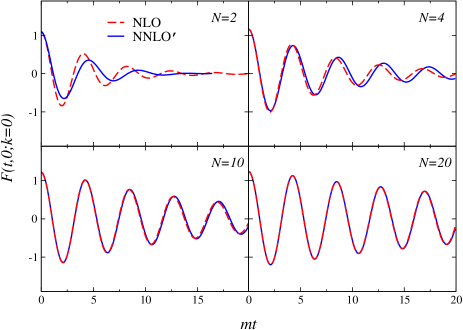
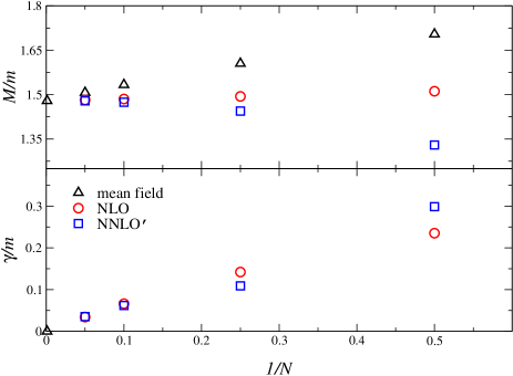
The unequal-time two-point function at zero momentum is shown in Fig. 2. The coupling is $\lambda/m^{2}=30$, where $m$ is the renormalized mass in vacuum. The lattice spacing is $am=0.5$ and volume $Lm=32$. The memory kernel is preserved completely. At LO (not shown) there is no damping in the unequal-time correlation function. Beyond LO, we observe an underdamped oscillation, the signal of a well-defined quasiparticle. Increasing $N$ shows convergence of the two truncations considered. We can extract the quasiparticle properties far from equilibrium by fitting these curves to an Ansatz of the form $Ae^{-\gamma t}\cos Mt$, where $M$ is the quasiparticle mass and $\gamma$ its width (divided by 2). The resulting values are shown in Fig. 3 as a function of $1/N$. We observe effective convergence when the value of $N$ is increased, as expected for a controlled expansion. For $N\gtrsim 10$, the NLO and N²LO^′ results are practically indistinguishable. In $1+1$ dimensions the perturbative onshell width from $2\to 2$ scattering processes is not defined due to the constraints from energy-momentum conservation. However, including higher order effects via the use of selfconsistently determined propagators leads to a width that vanishes as $1/N$, as expected from naive powercounting. The quasiparticle mass converges to the value determined by the nonthermal fixed point of the mean field equations in the large $N$ limit, which can be computed analytically Aarts:2000wi . For the parameters used here we find $M/m=1.48$ when $N\to\infty$.

Figure 3: Masses and widths extracted from the unequal-time correlation functions in Fig. 2 as a function of $1/N$. In the mean field approximation, the width is zero for all values of $N$.

Classical statistical field theory – In order to further investigate the applicability of the $1/N$ expansion and in particular the role of the 4-loop diagram at N²LO, we turn to classical statistical field theory, where the nonperturbative evolution can be computed by numerically solving the classical field equations, sampling initial conditions from the Gaussian ensemble. In order to carry out the comparison, we also take the classical limit in the set of 2PI equations. In this limit statistical ($F$) two-point functions dominate with respect to spectral ($\rho$) functions. There are several ways this can be motivated, using for instance classical statistical diagrams or arguing for classicality when occupation numbers are large Aarts:1997kp ; Aarts:2001yn ; Cooper:2001bd . The result is that terms are dropped that are subleading when $F$ is taken to be much larger than $\rho$. For example, both in Eq. (6) at NLO and in Eq. (7) at N²LO, the last terms are dropped with respect to the first ones. We have carried out this procedure for all terms appearing in self energies at N²LO^′ in Ref. Aarts:2006cv .

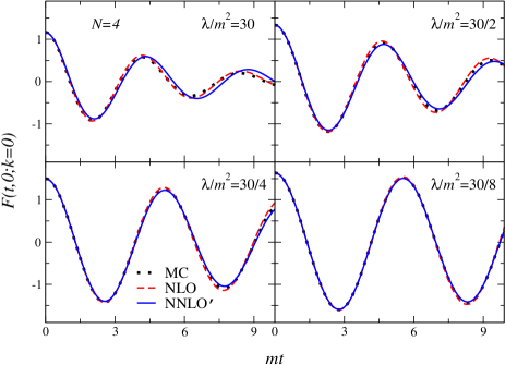
Since the 4-loop diagram at N²LO is suppressed by the coupling constant, its effect is expected to diminish at weaker coupling. In order to verify this, we use a relatively small value of $N=4$, where NLO and N²LO^′ differ at large coupling, both in the quantum and the classical theory. A comparison between NLO, N²LO^′, and the exact numerical result (MC for Monte Carlo) is shown in Fig. 4. In the numerical integration of the classical equations of motion, we have used a sample of $2.5\times 10^{5}$ initial conditions. In the top left corner, the coupling constant is $\lambda/m^{2}=30$. Damping at N²LO^′ is less than at NLO, similar to the situation in the quantum theory. Decreasing the coupling constant, we observe that the agreement between the two 2PI truncations improves. Moreover, for weaker coupling, we note that the MC results lie between the curves at NLO and N²LO^′, signalling a well converging expansion. For even smaller coupling (not shown), we found that all curves lie on top of each other, even for $N=4$. Since the N²LO approximation is numerically substantially more intensive than the NLO one, we have investigated whether the memory kernel at N²LO could be truncated earlier than at NLO, saving considerable computer resources. However, we found this not to be the case: in the results shown here it was necessary to preserve memory kernels over the entire history, also for the N²LO contribution. At this moment this prevents us from going to larger times and studying the approach to equilibrium beyond NLO.

Figure 4: Unequal time correlation function $F(t,0;{\mathbf{k}}={\bf 0})$ for $N=4$ in the classical theory. Included are the NLO and N²LO^′ results in the classical limit of the 2PI-$1/N$ expansion, and the exact result obtained by numerical integration of the classical equations of motion (MC). The coupling constant is $\lambda/m^{2}=30/n$, with $n=1,2,4,8$.

Summary – We have investigated convergence properties of the 2PI-$1/N$ expansion for nonequilibrium quantum fields. We included contributions at N²LO, and found that the expansion is convergent even at large coupling as $N$ is increased. At fixed $N$, we found convergence as the coupling strength is reduced. These results confirm that the 2PI-$1/N$ expansion truncated at NLO already gives quantitatively accurate results for moderate values of $N$ or coupling strength: At any coupling $N=10$ works very well, whereas for the often used $N=4$, a trade-off in terms of a smaller coupling is required for precision calculations. We expect this behaviour to persist in $3+1$ dimensions, but a direct confirmation would be welcome.