x Reparametrization Invariant Collinear Operators

Abstract

In constructing collinear operators, which describe the production of energetic jets or energetic hadrons, important constraints are provided by reparametrization invariance (RPI). RPI encodes Lorentz invariance in a power expansion about a collinear direction, and connects the Wilson coefficients of operators at different orders in this expansion to all orders in $\alpha_{s}$. We construct reparametrization invariant collinear objects. The expansion of operators built from these objects provides an efficient way of deriving RPI relations and finding a minimal basis of operators, particularly when one has an observable with multiple collinear directions and/or soft particles. Complete basis of operators are constructed for pure glue currents at twist-4, and for operators with multiple collinear directions, including those appearing in $e^{+}e^{-}\to 3\,{\rm jets}$, and for $pp\to 2\,{\rm jets}$ initiated via gluon-fusion.

I Introduction

Factorization theorems play a crucial role in our understanding of QCD Collins et al. (1988); Sterman (1995). For processes with large momentum transfer or energy release they provide a separation of the high-energy perturbative contributions from the low energy process independent functions describing non-perturbative dynamics. The soft-collinear effective theory (SCET) provides a systematic approach to the separation of hard, soft, and collinear dynamics in processes with energetic hadrons or jets Bauer et al. (2001a, b); Bauer and Stewart (2001); Bauer et al. (2002a). It has an operator based approach to hard-collinear factorization which provides a simple framework for deriving the convolution formulae connecting Wilson coefficients and collinear operators. The hard Wilson coefficients describe the short distance process dependent contributions, and the operators built out of collinear and soft fields encode the longer distance hadronization into individual energetic hadrons, energetic jets, or hadrons with soft momenta. With more than one collinear direction the factorization for SCET operators was first considered in Ref. Bauer et al. (2002b), and it was demonstrated that the leading order operators efficiently encode traditional factorization theorems for processes like Deep-Inelastic Scattering (DIS), Drell-Yan, Deeply-Virtual Compton Scattering (DVCS), and exclusive form factors with hard momentum transfer. Compared to more traditional methods, an advantage of the effective theory approach to high-energy factorization is the systematic description of power corrections by higher order operators and effective Lagrangians Chay and Kim (2002); Beneke et al. (2002); Hill and Neubert (2003); Bauer et al. (2003a).

An important constraint on the construction of both leading and power suppressed operators in SCET is provided by reparametrization invariance (RPI). The utility of reparametrization invariance was first discussed in Ref. Luke and Manohar (1992) in the context of heavy quark effective theory (HQET). In HQET there are 3 generators for RPI, and the transformations involve a time-like vector $v^{\mu}$ where $v^{2}=1$. For collinear operators in SCET, RPI transformations act on null vectors $n^{\mu}$ and ${\bar{n}}^{\mu}$ where $n\!\cdot\!{\bar{n}}=2$ and there are 5 generators for each type of collinear field. Reparametrization invariance in SCET was first discussed in Ref. Chay and Kim (2002) and generalized to the complete set of RPI transformations in Ref. Manohar et al. (2002).

To see how reparametrization constraints come about, let’s consider a process with multiple energetic jets defined by an infrared safe jet algorithm, as pictured in Fig. -1379. We assign labels $n_{1}^{\mu}$, $n_{2}^{\mu}$, $n_{3}^{\mu}$, $\ldots$ to the jets, which are null $n_{i}^{2}=0$, and whose vector components identify the directions $\vec{n}_{i}$ of the total momentum vector of all hadrons in the jet. The hadronization in each jet takes place in a collinear cone about each $\vec{n}_{i}$, and we refer to the energetic particles in this jet as $n_{i}$-collinear. Interactions between particles in different jets can take place only by hard exchange at short distance or by soft exchange at long distance. The description of the physics of a jet is simplified by a suitable set of coordinates, which are provided by $n_{i}^{\mu}$, and a complementary null vector ${\bar{n}}_{i}^{\mu}$ where ${\bar{n}}_{i}^{2}=0$ and $n_{i}\!\cdot\!{\bar{n}}_{i}=2$. The momentum of a particle in the $i$’th jet can be decomposed in these coordinates as

$$p^{\mu}=n_{i}\!\cdot\!p\>\frac{{\bar{n}}_{i}^{\mu}}{2}+{\bar{n}}_{i}\!\cdot\!p\>\frac{n_{i}^{\mu}}{2}+p_{n_{i}\perp}^{\mu}\,.$$ (1)

The collinear modes for the jet have momentum scaling as $(n_{i}\cdot p,{\bar{n}}_{i}\cdot p,p_{n_{i}\perp})\sim Q(\lambda^{2},1,\lambda)$ where $\lambda\ll 1$ and $Q^{2}$ is a large perturbative momentum scale (the jet-energy). In cases where our discussion is generic to any one jet we will leave off the subscript $i$, so $n_{i}\to n$ and ${\bar{n}}_{i}\to{\bar{n}}$. The definition of $\perp$ in Eq. (1) is relative to $n$ and ${\bar{n}}$, and for this reason we use the notation $p_{n\perp}^{\mu}$, with $n\!\cdot\!p_{n\perp}={\bar{n}}\!\cdot\!p_{n\perp}=0$. When it is clear which $n$ and ${\bar{n}}$ we are referring to we will sometimes write $p_{\perp}^{\mu}$ for $p_{n\perp}^{\mu}$. For each $n$, collinear operators are built up from quark $\xi_{n}$ and gluon $A_{n}^{\mu}$ fields, which are labeled by their collinear direction, and describe quantum fluctuations close to the direction $n$ with offshellness $p^{2}\ll Q^{2}$. Two collinear directions are described by distinct collinear fields when $n_{i}\cdot n_{j}\gg\lambda^{2}$ for $i\neq j$ Bauer et al. (2002b). In Eq. (1) ${\bar{n}}_{i}$ is introduced solely to provide a basis vector for the decomposition, unlike $n_{i}$ which has a physical association. For multiple collinear directions we have the freedom to introduce multiple ${\bar{n}}_{i}^{\mu}$ vectors.

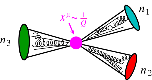
Figure -1379: Three collinear jets labeled by vectors $n_{i}^{\mu}$.

Reparametrization constraints arise because the decomposition in Eq. (1) is not unique. We can shift $n_{i}$ by a small amount and still have a suitable basis vector for the $i$’th jet. We also have a large amount of freedom in the choice of ${\bar{n}}_{i}$. For each $\{n,{\bar{n}}\}$ pair the most general set of RPI transformations which preserves the relations $n^{2}=0$, $\bar{n}^{2}=0$, and $n\!\cdot\!\bar{n}=2$ are

$$\text{(I)}\left\{\begin{tabular}[]{l}$n_{\mu}\to n_{\mu}+\Delta_{\mu}^{\perp}$\\ $\bar{n}_{\mu}\to\bar{n}_{\mu}$\end{tabular}\right.\qquad\text{(II)}\left\{\begin{tabular}[]{l}$n_{\mu}\to n_{\mu}$\\ $\bar{n}_{\mu}\to\bar{n}_{\mu}+\varepsilon_{\mu}^{\perp}$\end{tabular}\right.\qquad\text{(III)}\left\{\begin{tabular}[]{l}$n_{\mu}\to(1+\alpha)\,n_{\mu}$\\ $\bar{n}_{\mu}\to(1-\alpha)\,\bar{n}_{\mu}$\end{tabular}\right.\,,$$ (8)

where the five infinitesimal parameters are $\{\Delta^{\bot}_{\mu},\epsilon^{\bot}_{\mu},\alpha\}$, and satisfy $\bar{n}\!\cdot\!\epsilon^{\bot}=n\!\cdot\!\epsilon^{\bot}=\bar{n}\!\cdot\!\Delta^{\bot}=n\!\cdot\!\Delta^{\bot}=0$. To ensure that $n$ provides an equivalent physical description of the collinear direction for these particles requires the power counting $\{\Delta^{\bot}_{\mu},\epsilon^{\bot}_{\mu},\alpha\}\sim\{\lambda^{1},\lambda^{0},\lambda^{0}\}$ Manohar et al. (2002). Thus $n$ can only be shifted by a small amount, while parametrically large values of $\alpha$ and $\varepsilon^{\bot}_{\mu}$ are allowed. In B-meson decays, constraints from reparametrization invariance in SCET have been derived for heavy-to-light currents with parameters $v$ and $n$, at the first subleading order in Refs. Chay and Kim (2002); Beneke et al. (2002); Pirjol and Stewart (2003), and to second order in Ref. Arnesen et al. (2005). Results for light-light SCET currents with one collinear direction $n$, were derived at first subleading order in Ref. Hardmeier et al. (2004). The extension of RPI relations to collinear operators involving light quark masses was developed in Ref. Chay et al. (2005a).

The goal of our paper is to provide a simple procedure for constructing the RPI-completion of operators $O(n_{i},{\bar{n}}_{i},v_{i})$ that depend on multiple light-like vectors $\{n_{i},{\bar{n}}_{i}\}$ and time-like vectors $v_{i}$. The procedure should be sufficiently general to be used for any hard-scattering process, and also easy to extend to any desired order in the twist or $\lambda$ expansion. To achieve this we must deal with a technical obstacle: so far all applications of RPI to hard-scattering in the SCET and in other factorization literature have constructed a complete basis of operators first and then dealt with deriving connections between the operators order by order in the $\lambda$ expansion. This approach quickly becomes cumbersome at higher orders or when dealing with operators with multiple directions. For example, in this approach the RPI completion of a basis of three jet operators $O(n_{1},n_{2},n_{3},{\bar{n}}_{1},{\bar{n}}_{2},{\bar{n}}_{3})$, would require studying three copies of Eq. (8) or nine transformations.

For cases with multiple time-like vectors, an alternative approach is known from HQET Manohar et al. (2002). Here an RPI heavy quark field is constructed at the beginning, $H_{v}$, which has an expansion that starts with the standard HQET field, $H_{v}=h_{v}+\ldots$. A basis of reparametrization invariant operators built from $H_{v}$ automatically encodes the RPI relations at any order in the power expansion, and when expanded generates a series of operators with connected Wilson coefficients. In this paper we develop a suitable set of RPI and gauge invariant objects for SCET. These objects include a quark field operator $\Psi_{n}$, a gluon field strength operator ${\cal G}_{n}^{\mu\nu}$, and $\delta$-function operators which pick out the large momenta of collinear fields. The gauge invariance of these objects is ensured using a “reparametrization invariant Wilson line” operator ${\cal W}_{n}$. These objects allow us to extend the invariant operator procedure to processes that depend on null-vectors.

In hard-scattering processes, DIS provides a familiar context where the construction of a minimal operator basis requires judicial use of the quark and gluon equations of motion, and an invariance under reparametrizations of a light-like direction Politzer (1980); Jaffe and Soldate (1981, 1982); Ellis et al. (1982, 1983), for a review see Jaffe (1996). The invariance under reparametrizations becomes more valuable at higher orders in the expansion, being particularly constraining on the basis of twist-4 operators derived in

Refs. Jaffe and Soldate (1981, 1982); Ellis et al. (1982, 1983). We derive RPI constraints for collinear operators in DIS and compare to these classic results as a test of our setup. For DIS the minimization of the basis of RPI operators is quite similar to the reduction of operators in Ref. Jaffe and Soldate (1982). On the other hand the basis of SCET operators are comprised entirely of analogs of “good” quark and gluon fields, namely a two-component quark field $\chi_{n}$ and just two components of the gluon field strength, ${\cal B}_{n\perp}^{\mu}$. These objects both incorporate Wilson lines, and for these operators it is easier to find a minimal basis. The RPI relations provide Lorentz invariance connections between the Wilson coefficients in this basis. These constraints carry a process independence, they depend on the type of operators being considered, but not on the precise process in which they will be used. It should be emphasized that when matrix elements are considered for a particular process, a further reduction in the number of independent hadronic functions becomes possible. For twist-4 quark operators in DIS this type of further reduction was discussed in detail in Ref. Ellis et al. (1983) and for inclusive B-decays in. Tackmann (2005), but this type of reduction is not our focus here.

Our construction is general enough that it applies not just to DIS like processes, but to operators with multiple collinear directions, which are useful for processes with multiple hadrons and jets. These operator bases provide a starting point for deriving appropriate factorization theorems for different processes. The invariant operator procedure becomes more and more efficient as the number of directions grows.

The outline of our paper is as follows. In section II we review ingredients from SCET needed for our analysis. We divide hard interactions into two categories, those with an external hard leptonic reference vector $q^{\mu}$, and those where the hard interaction is between strongly interacting particles. Since most SCET applications focus on the former case, we address some of the additional notational complications that occur for the latter. Section III introduces a formalism for using reparametrization invariant objects in SCET. A set of RPI invariant collinear objects is constructed in section III.1, followed by a summary of identities that can be used to reduce the operator basis in section III.2. The inclusion of mass effects is considered in section III.3, and the expansion of the RPI objects is carried out in section III.4. Applications for constructing operators are considered in section IV. In section IV.1 we verify that our approach provides a simple way to reproduce the known RPI result for the chiral-even scalar current given in Ref. Hardmeier et al. (2004). In section IV.2 we construct a general basis of field structures involving up to four active quark or gluon operators, and with up to four distinct collinear directions. In section IV.3 we consider the special case of quark operators for DIS at twist-4 with one collinear direction, and compare with the literature. In section IV.4 we derive a basis of operators for pure gluon scattering in DIS up to twist-4. Finally we apply the formalism to jet production. In section IV.5 we demonstrate that very little information is gained about the operator basis describing $e^{+}e^{-}\to 2\,{\rm jets}$. In section IV.6 we show that RPI turns out to be quite powerful for constraining the $e^{+}e^{-}\to 3\,{\rm jet}$ operators. Finally we show that RPI is also useful for two jet production from gluon-fusion, $gg\to q\bar{q}$, and we construct a basis of operators for this process in section IV.7. Conclusions are given in section V.

II Review of SCET

In sections II.1 and II.2 below, we introduce some basic definitions and properties of SCET that we will need for our computations. In section II.3 a brief review of the null and time-like RPI transformations is given, and in section II.4 a review of hard-collinear convolutions is given since they play an important role in subsequent sections.

II.1 Fields, Wilson lines, and Power Counting

SCET fields include collinear gluons $A_{n}^{\mu}$ and collinear quarks $\xi_{n}$ for each distinct direction $n$. An important attribute of the collinear fields is that they carry both a large label momentum $p$ and a coordinate $x$, such as $\xi_{n,p}(x)$. The label momenta are picked out by momentum operators, $\overline{\mathcal{P}}_{n}\xi_{n,p}={\bar{n}}\!\cdot\!p\,\xi_{n,p}$ and ${\mathcal{P}}_{n\perp}^{\mu}\xi_{n,p}=p_{\perp}^{\mu}\xi_{n,p}$, while derivatives $i\partial^{\mu}$ act on the coordinate $x$ and scale as $i\partial^{\mu}\sim\lambda^{2}$ (see Ref. Bauer and Stewart (2001)). Having two types of derivatives makes it simple to couple collinear and ultrasoft particles for ${\rm SCET}_{\rm I}$, including ultrasoft gluons $A_{us}^{\mu}$ and quarks $q_{us}$, and when appropriate, heavy quarks $h_{v}^{us}$ as well. The soft fields for ${\rm SCET}_{\rm II}$ are $A_{s}^{\mu}$, $q_{s}$, and a heavy quark $h_{v}^{s}$.

We define collinear covariant derivatives as

$$i\bar{n}\!\cdot\!D_{n}=\overline{\mathcal{P}}_{n}+g\bar{n}\!\cdot\!A_{n,p}\,,\qquad iD_{n}^{\perp\mu}=\mathcal{P}_{n\bot}^{\mu}+gA_{n,p}^{\perp\mu}\,,\qquad in\!\cdot\!D_{n}=in\!\cdot\!\partial+gn\!\cdot\!A_{n,p}\,.$$ (9)

When integrating out hard offshell fluctuations and constructing gauge invariant structures in SCET, it is necessary to include collinear Wilson lines, $W_{n}$, defined by

$$W_{n}(x) = \Big{[}\sum_{\textrm{perms}}\exp\Big{(}\frac{-g}{\overline{\mathcal{P}}}\>\bar{n}\!\cdot\!A_{n,p}(x)\>\Big{)}\Big{]}\,.$$ (10)

The collinear fields $A_{n,p}^{\mu}$ are defined with the zero-bin procedure Manohar and Stewart (2007). To couple ultrasoft degrees of freedom we define an ultrasoft covariant derivative

$$iD_{us}^{\mu}=i\partial^{\mu}+gA_{us}^{\mu}\,,$$ (11)

that can act on collinear fields. At lowest order the coupling to $n$-collinear fields involves $n\!\cdot\!D_{us}$ and can be removed from the Lagrangian by the BPS field redefinition Bauer et al. (2002a)

$$\xi_{n,p}(x)\to Y_{n}(x)\xi_{n,p}(x)\,,\qquad A_{n,q}(x)\to Y_{n}(x)A_{n,q}(x)Y_{n}^{\dagger}(x)\,,$$ (12)

with the ultrasoft Wilson line

$$Y_{n}(x^{\mu})={\rm P}\exp\Big{(}i\,g\int^{0}_{-\infty}\!\!ds\ n\!\cdot\!A_{us}(x^{\mu}+sn^{\mu})\Big{)}\,.$$ (13)

This field redefinition allows us to organize power corrections as gauge invariant products of collinear and ultrasoft fields as we discuss in the next section. In describing $e^{+}e^{-}\to{\rm jets}$ in SCET it is convenient to make a field redefinition with Wilson lines over $(0,\infty)$ rather than the $Y_{n}$ shown in Eq. (13) Bauer et al. (2004); Chay et al. (2005b). For $q\bar{q}\to{\rm jets}$ one can use lines over $(0,\infty)$ or $(-\infty,0)$. The final results are always independent of the choice of the reference point for $Y$ in the field redefinition (the $-\infty$ in Eq. (13)) since it does not dictate the direction of the lines in the final result Arnesen et al. (2005) (though the same choice should be used in all parts of the computation).

Operators are formed from products of the above fields, and the power counting for an operator is determined by adding up contributions from its constituents. The power counting for the fields and derivatives in ${\rm SCET}_{\rm I}$ is

$$\ \xi_{n}\sim\lambda, (n\!\cdot\!A_{n},{\bar{n}}\!\cdot\!A_{n},A_{n}^{\perp}) \sim(\lambda^{2},1,\lambda)\,, q_{us} \sim h_{v}^{us}\sim\lambda^{3}, A_{us} \sim\lambda^{2}\,,$$

$$i\partial^{\mu}\sim\lambda^{2}\,, (in\!\cdot\!\partial,{\bar{n}}\!\cdot\!{\mathcal{P}},{\mathcal{P}}_{n\perp}) \sim(\lambda^{2},1,\lambda)\,, W_{n} \sim Y_{n}\sim\lambda^{0}\,.$$ (14)

Here the ultrasoft fields describe fluctuations with offshellness much less than the collinear particles. These objects can be used to construct operators for processes with multiple jets. For a collinear jet we have $\lambda\sim\Delta/Q$ with $\Lambda_{\rm QCD}\ll\Delta\ll Q$. For a collinear hadron we have a smaller $\lambda$, namely $\lambda\sim\Lambda_{\rm QCD}/Q$. For processes with two or more hadrons the interactions in the theory ${\rm SCET}_{\rm II}$ must be considered. With a small parameter $\eta\sim\Lambda_{\rm QCD}/Q\ll 1$ the power counting of fields in this theory are

$$\ \xi_{n}\sim\eta, (n\!\cdot\!A_{n},{\bar{n}}\!\cdot\!A_{n},A_{n}^{\perp}) \sim(\eta^{2},1,\eta)\,, q_{s} \sim h_{v}^{s}\sim\eta^{3/2}, A_{s} \sim\eta\,,$$

$$i\partial_{s}^{\mu}\sim\eta\,, (in\!\cdot\!\partial,{\bar{n}}\!\cdot\!{\mathcal{P}},{\mathcal{P}}_{n\perp}) \sim(\eta^{2},1,\eta)\,, W_{n} \sim S_{n}\sim\eta^{0}\,.$$ (15)

Here the soft fields describe fluctuations with similar offshellness to the collinear fields. In cases with jets and energetic hadrons a succession of ${\rm SCET}_{\rm I}$ and ${\rm SCET}_{\rm II}$ theories needs to be considered.

Our article focuses on building reparametrization invariant operators from products of collinear fields that describe an underlying hard interaction, since this is the most involved part of the construction. The simple strategy we follow to incorporate “ultrasoft” and “soft” fields into the analysis is summarized in sections II.2 and II.3 below.

II.2 Gauge Invariant Field Products and Convolutions

To build operators in SCET we want to use structures which are gauge invariant and homogeneous in the power counting. Although the precise manner in which the Wilson lines $W_{n}$ appears is determined by matching, and the precise manner in which Wilson lines $Y_{n}$ appear is determined by ultrasoft-collinear factorization, some general structures can be identified. For ${\rm SCET}_{\rm I}$ a convenient set of structures are:

$$\chi_{n}\equiv W_{n}^{\dagger}\xi_{n},\qquad{\mathcal{D}}_{n}^{\mu}\equiv W_{n}^{\dagger}D_{n}^{\mu}W_{n}\,,$$ (16)

$$q_{us}^{n}\equiv Y_{n}^{\dagger}q_{us},\qquad{\mathcal{D}}_{us}^{n\mu}\equiv Y_{n}^{\dagger}D_{us}^{\mu}Y_{n}\,,\qquad{\mathcal{H}}_{v}^{n}\equiv Y_{n}^{\dagger}h_{v},$$

together with the ${\mathcal{P}}_{n}^{\mu}$ label momentum operator and derivative operator $i\partial^{\mu}$ acting on these gauge invariant structures. The collinear fields in Eq. (16) are the ones obtained after the field redefinition in Eq. (12). It is convenient to be able to switch the collinear derivatives multiplied by Wilson lines for gauge invariant field strengths, for which we use

$$i{\mathcal{D}}_{n}^{\!\perp\mu} = {\mathcal{P}}_{n\perp}^{\mu}+g\mathcal{B}_{\!n\bot}^{\mu}\,,\qquad\qquad\!\!\!i\overleftarrow{\mathcal{D}}_{n}^{\!\perp\mu}=-{\mathcal{P}}_{n\perp}^{\,\dagger\mu}-g\mathcal{B}_{\!n\bot}^{\mu}\,,$$

$$in\!\cdot\!{\mathcal{D}}_{n} = in\!\cdot\!\partial+gn\!\cdot\!\mathcal{B}_{n}\,,\qquad in\!\cdot\!\overleftarrow{\mathcal{D}}_{n}=in\!\cdot\!\overleftarrow{\partial}-gn\!\cdot\!\mathcal{B}_{n}\,,$$ (17)

and note that ${\bar{n}}\!\cdot\!{\cal D}_{n}=\bar{\mathcal{P}}_{n}$. Here the field strength tensors are

$$g\mathcal{B}_{\!n\bot}^{\mu}\equiv\Big{[}\frac{1}{\overline{\mathcal{P}}_{n}}[i\bar{n}\!\cdot\!{\mathcal{D}}_{n},i{\mathcal{D}}_{n}^{\perp\mu}]\Big{]}\,,\qquad\qquad gn\!\cdot\!\mathcal{B}_{n}\equiv\Big{[}\frac{1}{\overline{\mathcal{P}}_{n}}[i\bar{n}\!\cdot\!{\mathcal{D}}_{n},in\!\cdot\!{\mathcal{D}}_{n}]\Big{]},$$ (18)

where the label operators and derivatives act only on fields inside the outer square brackets, and $g{\cal B}_{n\perp}^{\mu}$ and $gn\!\cdot\!{\cal B}_{n}$ are Hermitian.

For ${\rm SCET}_{\rm II}$ with hadrons we have the same collinear invariant objects as in Eq. (II.4), and similar soft invariant objects, that are obtained by replacing the ultrasoft fields by their soft counterparts, ${\cal H}_{v}^{n}=(Y_{n}^{\dagger}h_{v}^{us})\to{\cal H}_{v}^{n}=(S_{n}^{\dagger}h_{v}^{s})$, ${\cal D}_{us}^{n\mu}\to{\cal D}^{n\mu}_{s}$, and $q_{us}^{n}=(Y_{n}^{\dagger}q_{us})\to q_{s}^{n}=(S_{n}^{\dagger}q_{s})$. The soft Wilson line $S_{n}^{\dagger}$ is generated by integrating out offshell fluctuations which determine its direction $n$, and outgoing/incoming boundary conditions. Most often these operators can be constructed by a matching calculation from ${\rm SCET}_{\rm I}$, in which case the properties of the soft Wilson lines are directly inherited from the ultrasoft ones in ${\rm SCET}_{\rm I}$ Bauer et al. (2003b), and the product of $C(Q^{2},\omega_{i})$ from Eq. (26) and $J(\omega_{i},k_{j})$ from Eq. (34) becomes the Wilson coefficient of the factorized operator in ${\rm SCET}_{\rm II}$. In this paper we focus on ${\rm SCET}_{\rm I}$ examples.

II.3 Reparametrization invariance

When a set of fields have their largest momentum component in a light-like or time-like direction then the structure of operators built from these fields is constrained by reparametrization invariance. This invariance appears due to the ambiguity in the decomposition of momenta in terms of basis vectors and in terms of large and small components. For a collinear momentum, the set of five transformations on the light-like basis vectors $n_{i}^{\mu}$ and ${\bar{n}}_{i}^{\mu}$ were given in Eq. (8). These infinitesimal changes preserve the relations $n_{i}^{2}=0$, $\bar{n}_{i}^{2}=0$, $n_{i}\!\cdot\!\bar{n}_{i}=2$, and with the power counting $\{\Delta^{\perp},\varepsilon^{\perp},\alpha\}\sim\{\lambda,\lambda^{0},\lambda^{0}\}$ can have no physical consequences on the description of an observable. The type-III boost simply ensures that $(\#Nn_{i})-(\#N{\bar{n}}_{i})-(\#Dn_{i})+(\#D{\bar{n}}_{i})=0$ for each $i$, where $(\#Nn_{i})$ counts the number of $n_{i}$ factors in the numerator of an operator, $(\#D{\bar{n}}_{i})$ counts the numbers of ${\bar{n}}_{i}$ factors in the denominator, etc. With three collinear directions an example of a type-III RPI invariant parameter is

$$\frac{n_{1}\!\cdot\!{\bar{n}}_{2}\ {\bar{n}}_{1}\!\cdot\!{\bar{n}}_{3}}{{\bar{n}}_{2}\!\cdot\!{\bar{n}}_{3}}\,.$$ (19)

The type-I and type-II transformations of collinear objects are more interesting and are summarized in Table 1, which we take from Ref. Manohar et al. (2002). Since the factors induced by these transformations occur at different orders in $\lambda$, demanding overall invariance of a physical process provides connections between the Wilson coefficients of operators at different orders in the expansion.

Type (I)			Type (II)
$n$	$\to$	$n+\Delta^{\perp}$	$n$	$\to$	$n$
${\bar{n}}$	$\to$	${\bar{n}}$	${\bar{n}}$	$\to$	${\bar{n}}+\varepsilon^{\perp}$
$n\!\cdot\!D_{n}$	$\to$	$n\!\cdot\!D_{n}+\Delta^{\perp}\!\cdot\!D_{n}^{\perp}$	$n\!\cdot\!D_{n}$	$\to$	$n\!\cdot\!D_{n}$
$D_{n\perp}^{\mu}$	$\to$	$D_{n\perp}^{\mu}-\mbox{\large$\frac{\Delta_{\perp}^{\mu}}{2}$}\>{\bar{n}}\!\cdot\!D_{n}-\mbox{\Large$\frac{{\bar{n}}^{\mu}}{2}$}\Delta^{\perp}\!\cdot\!D_{n\perp}$	$D_{n\perp}^{\mu}$	$\to$	$D_{n\perp}^{\mu}-\mbox{\Large$\frac{\varepsilon_{\perp}^{\mu}}{2}$}\,\>n\!\cdot\!D_{n}-\mbox{\Large$\frac{n^{\mu}}{2}$}\,\varepsilon^{\perp}\!\!\cdot\!D_{n}^{\perp}$
${\bar{n}}\!\cdot\!D_{n}$	$\to$	${\bar{n}}\!\cdot\!D_{n}$	${\bar{n}}\!\cdot\!D_{n}$	$\to$	${\bar{n}}\!\cdot\!D_{n}+\varepsilon^{\perp}\!\cdot\!D_{n}^{\perp}$
$\xi_{n}$	$\to$	$\left(1+\frac{1}{4}\,\Delta\!\!\!/^{\perp}\bar{n}\!\!\!/\right)\xi_{n}$	$\xi_{n}$	$\to$	$\left(1+\frac{1}{2}\,\varepsilon\!\!\!/^{\perp}\frac{1}{\textstyle{\bar{n}}\!\cdot\!D_{n}}\>{D\!\!\!\!/}\,{}_{n}^{\perp}\right)\,\xi_{n}$
$W$	$\to$	$W$	$W$	$\to$	$\Big{[}\big{(}1-\frac{1}{\textstyle{\bar{n}}\!\cdot\!D_{n}}\,\,\epsilon^{\perp}\!\cdot\!D_{n}^{\perp}\big{)}W\Big{]}$

Table 1: Summary of infinitesimal type I and II transformations from Ref. Manohar et al. (2002). With multiple collinear directions these transformations exist for each $\{n_{i},{\bar{n}}_{i}\}$ pair.

When we couple collinear and ultrasoft particles there is another ambiguity, associated with the decomposition of a collinear momentum into large and small pieces. If the total momentum $P^{\mu}$ of a collinear particle is decomposed into the sum of a large collinear $p^{\mu}$ and a small ultrasoft momentum $k^{\mu}$:

$$P^{\mu} = p^{\mu}+k^{\mu}=\frac{n^{\mu}}{2}\bar{n}\!\cdot\!(p+k)+\frac{\bar{n}^{\mu}}{2}n\!\cdot\!k+(p_{\bot}+k_{\bot})^{\mu},$$ (20)

then operators must be invariant under a transformation that takes ${\bar{n}}\!\cdot\!p\to{\bar{n}}\!\cdot\!p+{\bar{n}}\!\cdot\!\ell$, $p_{\perp}^{\mu}\to p_{\perp}^{\mu}+\ell_{\perp}^{\mu}$, ${\bar{n}}\!\cdot\!k\to{\bar{n}}\!\cdot\!k-{\bar{n}}\!\cdot\!\ell$, and $k_{\perp}^{\mu}\to k_{\perp}^{\mu}-\ell_{\perp}^{\mu}$. To construct invariant objects that have nice gauge transformation properties we use the combined covariant derivatives Bauer et al. (2003a); Beneke and Feldmann (2003),

$$iD_{n\perp}^{\mu}+W_{n}iD_{us\perp}^{\mu}W_{n}^{\dagger}\,, i{\bar{n}}\!\cdot\!D_{n}+W_{n}i{\bar{n}}\!\cdot\!D_{us}W_{n}^{\dagger}\,.$$ (21)

This can be implemented by taking

$$i{\cal D}_{n\perp}^{\mu}\to i{\rm D}_{\rm full}^{\perp\mu}=i{\cal D}_{n\perp}^{\mu}+iD_{\rm us}^{\perp\mu}\,,\qquad\overline{\mathcal{P}}_{n}\to i{\bar{n}}\!\cdot\!{\rm D}_{\rm full}=\overline{\mathcal{P}}_{n}+i{\bar{n}}\!\cdot\!D_{\rm us}\,,$$ (22)

and then expanding in $\lambda$. The results in Eq. (22) give powerful relations as they relate the coefficients of operators involving collinear fields to those involving ultrasoft fields. These relations are quite easy to derive order by order in $\lambda$. Note that reparametrization constraints associated with transformation of the ultrasoft Wilson line $Y_{n}$ are automatically enforced by the other constraints.

Finally we review RPI for a time-like vector from HQET Luke and Manohar (1992). The momentum $P^{\mu}$ of a heavy quark is decomposed as $P^{\mu}=mv^{\mu}+k^{\mu},$ where $m$ is the heavy quark’s mass, $v^{\mu}$ is its velocity, and $k^{\mu}$ is a residual momentum of order $m\lambda^{2}$. For an infinitesimal $\beta^{\mu}\sim\lambda^{2}$ with $v\!\cdot\!\beta=0$, the shifts

$$v^{\mu}\rightarrow v^{\mu}+\beta^{\mu}\quad\text{and}\quad k^{\mu}\rightarrow k^{\mu}-m\beta^{\mu},$$ (23)

can have no physical consequences. This implies invariance under the infinitesimal change $h_{v}\to h_{v}+\delta h_{v}$ with $\delta h_{v}=(im\beta\!\cdot\!x+\beta\!\!\!//2)h_{v}$. A superfield can be constructed which is invariant under the full transformation Luke and Manohar (1992)

$$H_{v}(x)=e^{-imv\cdot x}\bigg{[}\frac{1}{\sqrt{2}(1+v\!\cdot\!{\cal V}/|{\cal V}|)}\Big{(}1+\frac{/\!\!\!{\cal V}\,/\!\!\!v}{|{\cal V}|}\Big{)}\bigg{]}h_{v}(x)$$ (24)

where

$${\cal V}^{\mu} =v^{\mu}+iD_{\rm us}^{\mu}/m\,.$$ (25)

Using this superfield one can build operators $O=O[H_{v}(x),D^{\mu}]$ that are invariant under reparametrizations of the time-like vector. Here $H_{v}=e^{-imv\cdot x}[1+iD\!\!\!\!//(2m)+\ldots]h_{v}$ at the first non-trivial order. Note that for heavy quarks, no dynamic component of the momentum is the same size as the hard fluctuations, so there is no analog of the $\delta$-functions in Eq. (II.4). This is the main complication we face in constructing invariant operators in SCET. The closest one gets in HQET is when we have two auxiliary time-like vectors, $v$ and $v^{\prime}$, such as in $B\to D^{(*)}$ decays. Here the invariant Wilson coefficients must be functions $C({\cal V}\!\cdot\!{\cal V}^{\prime})$ Neubert (1994).

II.4 Convolutions

In the presence of collinear fields a hard interaction can introduce convolutions in variables $\omega_{i}$ between the perturbatively calculable Wilson coefficient $C(Q^{2},\omega_{i})$ and the matrix element of the collinear operators. In this case the amplitude, cross-section, or decay rate has the form

$$A=\int\![d\omega_{1}\cdots d\omega_{k}]\>C(Q^{2},\omega_{i})\>\langle O(\omega_{i})\rangle\,.$$ (26)

The convolutions occur because a component of the hard momentum and of one or more collinear momenta are ${\cal O}(\lambda^{0})$. The exchange of momentum between the hard and collinear components yields a convolution in variables $\omega_{i}$, where the number of such variables is constrained by gauge invariance and by momentum conservation in the matrix element. A gauge invariant momentum from the collinear fields can be picked out by a delta function acting on one of the collinear objects in Eq. (16), such as $[\delta(\omega-{\bar{n}}\!\cdot\!{\cal P}_{n})\chi_{n}]$, and traditionally in SCET a subscript notation is used for these products,

$$\chi_{n,\omega} \equiv\Big{[}\>\delta\big{(}\omega-\overline{\mathcal{P}}_{n}\big{)}\chi_{n}\Big{]}\,, (i{\cal D}^{\mu}_{n\perp})_{\omega} \equiv\Big{[}i{\cal D}_{n\perp}^{\mu}\,\delta\big{(}\omega-\overline{\mathcal{P}}_{n}^{\dagger}\big{)}\Big{]}\,,$$

$$(g\mathcal{B}_{n\perp}^{\mu})_{\omega} \equiv\Big{[}g\mathcal{B}_{n\perp}^{\mu}\>\delta\big{(}\omega-\overline{\mathcal{P}}_{n}^{\dagger}\big{)}\Big{]}\,, (gn\!\cdot\!\mathcal{B}_{n})_{\omega} \equiv\Big{[}gn\!\cdot\!\mathcal{B}_{n}\>\delta\big{(}\omega-\overline{\mathcal{P}}_{n}^{\dagger}\big{)}\Big{]}\,.$$ (27)

We will refer to these as homogeneous objects since they have a definite order in $\lambda$, and call the operators build from these objects homogeneous operators. As an example we have the bilinear scalar operator,

$$O(\omega_{1},\omega_{2})=\bar{\chi}_{n,\omega_{1}}\,\frac{\bar{n}\!\!\!/}{2}\,\chi_{n,\omega_{2}}\,.$$ (28)

When we consider RPI it will be convenient to use different $\delta$ functions and convolution variables $\hat{\omega}$, that are type-III invariant. Essentially each $\overline{\mathcal{P}}_{n}={\bar{n}}\!\cdot\!{\cal P}_{n}$ must be multiplied by a scalar transforming as $n$ under RPI type-III. There are two cases to consider:

• situations where there is a reference vector $q^{\mu}$ for the hard interaction, $|q^{2}|=Q^{2}\gg\Lambda_{\rm QCD}$, which is external to the QCD dynamics,

• situations where the hard interactions are purely from strongly interacting particles.

Case i) applies to examples such as DIS where $q^{\mu}$ is the momentum transfer from the virtual photon, or $e^{+}e^{-}\to\ {\rm jets}$ where $q^{\mu}$ is the four momentum of the $e^{+}e^{-}$ pair. Here we can use $n\!\cdot\!q\sim\lambda^{0}$ to make the $\delta$-function type-III invariant for $n$-collinear fields. Since $Q^{2}\gg\Delta\Lambda_{\rm QCD}\gg\Lambda_{\rm QCD}^{2}$ we know that $n\!\cdot\!q\gg n\!\cdot\!p$, where $p$ is the momentum of a collinear particle in the jet. Thus we use a variable $\hat{\omega}$ with mass dimension two, and will find $\delta$-functions of the form

$$\delta\big{(}\hat{\omega}-n\!\cdot\!q\,\overline{\mathcal{P}}_{n}\big{)}\,.$$ (29)

We also introduce a subscript notation with hatted variables,

$$\chi_{n,\hat{\omega}} \equiv\Big{[}\>\delta\big{(}\hat{\omega}\!-\!n\!\cdot\!q\,\overline{\mathcal{P}}_{n}\big{)}\chi_{n}\Big{]}\,, (i{\cal D}^{\mu}_{n\perp})_{\hat{\omega}} \equiv\Big{[}i{\cal D}_{n\perp}^{\mu}\,\delta\big{(}\hat{\omega}\!-\!n\!\cdot\!q\,\overline{\mathcal{P}}_{n}^{\dagger}\big{)}\Big{]}\,,$$

$$(g\mathcal{B}_{n\perp}^{\mu})_{\hat{\omega}} \equiv\Big{[}g\mathcal{B}_{n\perp}^{\mu}\>\delta\big{(}\hat{\omega}\!-\!n\!\cdot\!q\,\overline{\mathcal{P}}_{n}^{\dagger}\big{)}\Big{]}\,, (gn\!\cdot\!\mathcal{B}_{n})_{\hat{\omega}} \equiv\Big{[}gn\!\cdot\!\mathcal{B}_{n}\>\delta\big{(}\hat{\omega}\!-\!n\!\cdot\!q\,\overline{\mathcal{P}}_{n}^{\dagger}\big{)}\Big{]}\,.$$ (30)

Since $\delta(\hat{\omega}-n\cdot q\overline{\mathcal{P}}_{n})\sim\lambda^{0}$, it is leading order in the power counting. Furthermore, we have $\delta(\hat{\omega}-n\cdot q\,\overline{\mathcal{P}})=\delta(\hat{\omega}/n\cdot q-\overline{\mathcal{P}})/n\cdot q$, so identifying $\hat{\omega}=n\!\cdot\!q\>\omega$ there is no real change to the structure of Eq. (26). An operator built out of the components given in Eq. (II.4) has multiple labels, $O(\hat{\omega}_{1},\hat{\omega}_{2},\ldots)$, and the Wilson coefficient for the operator will be a function of the same parameters, $C(\hat{\omega}_{1},\hat{\omega}_{2},\ldots)$, yielding Eq. (26) with $\hat{\omega}$’s replacing $\omega$’s.

For processes in case ii) there is no analog of the external $q^{\mu}$. Examples here include $pp\to{\rm jets}$, or any other hard process that does not involve external leptons or photons. The key difference with case i) is that here the hard interaction must involve two or more collinear directions, so we are guaranteed that there are scalar products $n_{i}\!\cdot\!n_{j}\sim\lambda^{0}$. For this type of reaction the type-III invariant $\delta$-functions which are convoluted with Wilson coefficients always involve large momenta for two different collinear directions,

$$\Delta_{ij}\equiv\delta\Big{(}\hat{\omega}_{ij}-\frac{1}{2}n_{i}\!\cdot\!n_{j}\,\overline{\mathcal{P}}_{n_{i}}\overline{\mathcal{P}}_{n_{j}}\Big{)}\,.$$ (31)

Here $\overline{\mathcal{P}}_{n_{i}}$ acts on a gauge invariant block of $n_{i}$-collinear fields, and $\overline{\mathcal{P}}_{n_{j}}$ acts on a block of $n_{j}$-collinear fields. Since this $\delta$-operator does not act on a single block of collinear fields we will not use a subscript notation like Eq. (II.4) for $\hat{\omega}_{ij}$. In this case the structure of the factorization theorem between operators and Wilson coefficients is a bit different than in Eq. (26). For example, consider an operator with collinear objects for four directions, where the convolution is

$$\int\big{[}\prod_{ij}\,d\hat{\omega}_{ij}\big{]}\>C(\hat{\omega}_{ij})[\prod_{km}\,\Delta_{km}]\ \bar{\chi}_{n_{1}}(g\mathcal{B}_{n_{3}}^{\perp})(g\mathcal{B}_{n_{4}}^{\perp})\chi_{n_{2}}\,.$$ (32)

Here the products are over the six unique pairs $ij$ with $i\neq j$, and $\overline{\mathcal{P}}_{n_{i}}$ in the $\Delta_{km}$ acts on the $n_{i}$-collinear field(s). The convolutions in Eq. (32) can be manipulated into the form of Eq. (26) by inserting four factors of $1=\int d\omega_{i}\>\delta(\omega_{i}-\overline{\mathcal{P}}_{n_{i}})$, writing $\hat{\delta}_{ij}=\delta(\hat{\omega}_{ij}-n_{i}\cdot n_{j}\,\omega_{i}\omega_{j}/2)$ and carrying out the integrals over the six $\hat{\omega}_{ij}$’s to give

$$\int\big{[}d\omega_{1}\cdots d\omega_{4}\big{]}\>C\big{(}n_{i}\!\cdot\!n_{j}\,\omega_{i}\omega_{j}\big{)}\bar{\chi}_{n_{1},\omega_{1}}(g\mathcal{B}_{n_{3},\omega_{3}}^{\perp})(g\mathcal{B}_{n_{4},\omega_{4}}^{\perp})\chi_{n_{2},\omega_{2}}\,.$$ (33)

Here the RPI-III transformation of the measure cancels against that of the $\delta$-functions in the operator, and RPI has constrained the Wilson coefficients to only depend on invariant products $n_{1}\!\cdot\!n_{2}\omega_{1}\omega_{2}$, $n_{1}\!\cdot\!n_{3}\omega_{1}\omega_{3}$, etc.

Due to the simplicity of the ultrasoft-collinear coupling at leading order in SCET a further factorization of the EFT matrix element can be made into collinear pieces $J$, and ultrasoft pieces $S$ at each order in the power counting:

$$\langle O(\omega_{i})\rangle=\int dk_{j}\>J(\omega_{i},k_{j})\>S(k_{j})\,.$$ (34)

However it is the factorization in Eq. (26) that will be central to our discussion of reparametrization invariant operators.

III Reparametrization Invariant Objects for SCET

To construct an expansion in operators in SCET the standard procedure is to build a gauge invariant basis of operators with definite power counting, order $\lambda^{k}$, and to assign a Wilson coefficient to each one. Afterwards one can impose RPI order by order and find relations among Wilson coefficients. On the contrary what we will do is to start with RPI and gauge invariant objects, to be constructed in section III.1. These objects do not have a definite power counting order, in particular we will know the order in the $\lambda$-expansion where they start, but they will contain terms at all higher orders as well. We build a basis with these RPI and gauge invariant objects, which is made minimal using equations of motion and kinematic constraints as discussed below in section III.2. (Equation of motion constraints for homogeneous operators are also summarized in this section.) Each element of this basis is assigned a Wilson coefficient, and then the elements are expanded to find the final basis with elements of a definite power counting. In this way we immediately obtain relations between Wilson coefficients of operators at different orders. Once we expand and check for redundancy, the number of independent Wilson coefficients is equal to the number of independent RPI operators in the reduced basis.

III.1 Construction of RPI and Gauge Invariant objects

We now construct reparametrization invariant objects in SCET whose leading terms give the fields in Eq. (II.1). These are then generalized to objects that are simultaneously RPI and gauge invariant whose leading terms give the objects in Eqs. (16,II.4). For simplicity only collinear objects are considered in this section. Pulling out the large phases from the collinear quark field and gluon field strength, and decomposing the full theory field into independent collinear sectors we have at tree level,

$$\psi(x)=\sum_{n}e^{-ix\cdot{\mathcal{P}}_{n}}\psi_{n}(x)\,,\qquad G^{\mu\nu}(x)=\sum_{n}e^{-ix\cdot{\mathcal{P}}_{n}}G_{n}^{\mu\nu}(x)\,.$$ (35)

Full Lorentz invariance act on the fields $\psi(x)$ and $G^{\mu\nu}(x)$, but the RPI transformations that we are interested acts independently on each collinear sector labeled by $n$. Two sectors $i$, $j$ are independent if $n_{i}\cdot n_{j}\gg\lambda^{2}$, and the sums in Eq. (35) are really over equivalence classes, $\{n\}$, where a class consists of vectors related by RPI. From the discussion in section II.3 the $n$-reparametrization invariant collinear quark and field strength are easy to identify

$$\psi_{n} \equiv \left(1+\frac{1}{{\bar{n}}\cdot D_{n}}/\!\!\!\!D_{n}^{\perp}\frac{{\bar{n}}\!\!\!/}{2}\right)\xi_{n}\,,\qquad\qquad ig\,G_{\mu\nu}^{n}\equiv\left[iD^{n}_{\mu},iD^{n}_{\nu}\right]\,.$$ (36)

Under the transformations in Table 1 for $\{n,{\bar{n}}\}$, the quark field $\psi_{n}$ remains invariant Manohar et al. (2002), while the gluon tensor is invariant because the vector $D_{n}^{\mu}$ is invariant. To make the fields in Eq. (36) invariant under the additional reparametrization transformations that link collinear and ultrasoft derivatives we replace $in\cdot D_{n}\to in\cdot D_{n}+gn\cdot A_{us}$, $iD_{n\perp}^{\mu}\to iD_{n\perp}^{\mu}+W_{n}iD_{us\perp}^{\mu}W_{n}^{\dagger}$, and $i{\bar{n}}\cdot D_{n}\to i{\bar{n}}\cdot D_{n}+W_{n}i{\bar{n}}\cdot D_{us}W_{n}^{\dagger}$. After this replacement the decoupling field redefinitions in Eq. (12) can be made. In Eq. (36) $n\!\!\!/\xi_{n}=0$, and the term in $\psi_{n}$ with a $\perp$-covariant derivative corresponds to the two components of the full fermion field that are small when $p_{\perp}/{\bar{n}}\cdot p\ll 1$. Since $n\!\!\!/\psi_{n}\neq 0$, the $\psi_{n}$ field does not provide a definite power counting for operators. For example, $\bar{\psi}_{n}\bar{n}\!\!\!/\psi_{n}\sim\lambda^{0}$ whereas $\bar{\psi}_{n}n\!\!\!/\psi_{n}\sim\lambda^{4}$.

We also need reparametrization invariant $\delta$-functions whose expansions reproduce Eqs. (29) and (31) at lowest order. For example, these are needed to construct an RPI operator which when expanded gives $\bar{\chi}_{n,\omega_{1}}\bar{n}\!\!\!/\chi_{n,\omega_{2}}$ at lowest order. For situations where there is an external hard vector $q^{\mu}$ the invariant $\delta$-function is

$$\hat{\Delta}_{i}\equiv\delta(\hat{\omega}-2q\cdot i\partial_{n_{i}}) =\delta(\hat{\omega}-n_{i}\!\cdot\!q\,\overline{\mathcal{P}}_{n_{i}})+\ldots\,,$$ (37)

where as described in section II.2, $q^{\mu}$ is a parameter specific to the kinematics of the process being studied. Notice that $\delta(\hat{\omega}-2q\cdot i\partial_{n})$ starts at ${\cal O}(\lambda^{0})$, is RPI, and is gauge invariant when acting on singlet operators. Here

$$i\partial_{n}^{\mu}\equiv\frac{n^{\mu}}{2}\overline{\mathcal{P}}_{n}+{\mathcal{P}}_{n\perp}^{\mu}+\frac{{\bar{n}}^{\mu}}{2}in\!\cdot\!\partial_{n}\,,$$ (38)

and functions of $i\partial_{n}^{\mu}\sim(\lambda^{2},1,\lambda)$ can be expanded in powers of $\lambda$. Note that $\overline{\mathcal{P}}_{n}$ and ${\mathcal{P}}_{n\perp}^{\mu}$ are only non-zero when they act on $n$-collinear fields. It is useful to extend this property to the full $i\partial_{n}^{\mu}$, which we can do by distributing an $i\partial^{\mu}$ derivative across all fields that it acts on, writing for example $i\partial^{\mu}\bar{\psi}_{n_{1}}\psi_{n_{2}}=(i\partial_{n_{1}}^{\mu}\bar{\psi}_{n_{1}})\psi_{n_{2}}+\bar{\psi}_{n_{1}}(i\partial_{n_{2}}^{\mu}\psi_{n_{2}})$. In some hard processes there is more than one external hard vector, and a natural question arises as to whether $q^{\mu}$ provides a unique choice for this construction. For example, in DVCS, $\gamma^{*}p\to\gamma^{(*)}p^{\prime}$ we have the momentum $q^{\mu}$ of the incoming $\gamma^{*}$ and the momentum $q^{\prime\mu}$ of the outgoing $\gamma^{(*)}$. In Appendix A we show that as long as $q_{\perp}-q^{\prime}_{\perp}\sim\lambda$ or smaller, the choice $q$ suffices, since for the purpose of constructing a basis of operators it is equivalent to the choice of any linear combination of $q$ and $q^{\prime}$. On the other hand, for situations where there is no external hard vector $q^{\mu}$, the appropriate RPI $\delta$-function is

$$\hat{\Delta}_{ij}\equiv\delta(\hat{\omega}_{ij}-2i\partial_{n_{i}}\cdot i\partial_{n_{j}})=\delta\Big{(}\hat{\omega}_{ij}-\frac{1}{2}n_{i}\cdot n_{j}\>\overline{\mathcal{P}}_{n_{i}}\overline{\mathcal{P}}_{n_{j}}\Big{)}+\ldots\,.$$ (39)

This $\delta$-function operator acts on two independent collinear directions. In general we must include in an operator a set of $\hat{\Delta}_{i}$ and $\hat{\Delta}_{ij}$ which are linearly independent. Once we expand, the first term in the series for $\hat{\Delta}_{ij}$ is not independent of the first term from $\hat{\Delta}_{i}$, so the $\delta$-function shown on the RHS of Eq. (39) can always be eliminated, as we did in Eq. (33).

We will also make use of a reparametrization invariant Wilson line, ${\cal W}_{n}$, which has the same gauge transformation properties as $W_{n}$,

$${\cal W}_{n}=W_{n}\>e^{-iR_{n}}\,.$$ (40)

Here the operator $R_{n}$ starts with a term at ${\cal O}(\lambda)$ and is built of $n$-collinear gluon fields,

$$R_{n}=R_{n}\big{[}\,\overline{\mathcal{P}}_{n}\,,{\mathcal{P}}_{n\perp}^{\mu}\,,g{\cal B}_{n\perp}^{\mu}\,,t^{\mu}\big{]}\,,$$ (41)

where the vector $t^{\mu}$ is either $q^{\mu}$ or $i\partial_{n^{\prime}}^{\mu}$ with $n\cdot n^{\prime}\sim\lambda^{0}$. Furthermore, $R_{n}$ is Hermitian, dimensionless, and collinear gauge invariant. We leave the explicit construction of $R_{n}$ to section III.4 below, and for the remainder of this section take these properties as given.

Under collinear gauge transformations, $\psi_{n}$ and ${\cal W}_{n}$ transform the same way as $\xi_{n}$ and $W_{n}$, and $G_{n}^{\mu\nu}$ transforms as a nonabelian field strength. Thus using ${\cal W}_{n}$ we can form analogs of the results in Eq. (II.4) that are simultaneously RPI and gauge invariant, namely the superfields

$$\Psi_{n}\equiv{\cal W}_{n}^{\dagger}\psi_{n}\,,\qquad{\cal G}^{\mu\nu}_{n}\equiv{\cal W}_{n}^{\dagger}G^{\mu\nu}_{n}{\cal W}_{n}\,.$$ (42)

For cases with an external $q^{\mu}$ we also introduce a subscript notation,

$$\Psi_{n,\hat{\omega}}\equiv\big{[}\delta(\hat{\omega}-2q\!\cdot\!i\partial_{n})\Psi_{n}\big{]}\,,\qquad{\cal G}^{\mu\nu}_{n,\hat{\omega}}\equiv\Big{[}{\cal G}^{\mu\nu}_{n}\,\delta(\hat{\omega}+2q\!\cdot\!i\,\overleftarrow{\partial_{n}})\Big{]}\,.$$ (43)

Operators built out of the superfields $\Psi_{n}$ and ${\cal G}_{n}^{\mu\nu}$ are simultaneously RPI and gauge invariant. They are not homogeneous in the power counting, but the superfields reduce to the objects in Eq. (II.4) at lowest order in the $\lambda$ expansion. For example, the superfield for the fermion

$$\Psi_{n} =e^{iR_{n}}\,W_{n}^{\dagger}\left(1+\frac{1}{i{\bar{n}}\cdot{D_{n}}}{iD_{n}}\!\!\!\!\!\!/^{\perp}\frac{{\bar{n}}\!\!\!/}{2}\right)\xi_{n}=e^{iR_{n}[i\partial_{n},{\cal B}_{n}]}\left(1+\frac{1}{\overline{\mathcal{P}}_{n}}i\mathcal{D}_{n}\!\!\!\!\!\!/^{\perp}\frac{{\bar{n}}\!\!\!/}{2}\right)\chi_{n}\,$$

$$=\chi_{n}+\ldots\,.$$ (44)

Similarly, $(g^{\perp}_{\nu\nu^{\prime}}{\bar{n}}_{\mu})ig({\cal G}^{\mu\nu^{\prime}}_{n})=\overline{\mathcal{P}}_{n}\,g{\cal B}_{n\nu}^{\perp}+\ldots$. Thus to form a RPI version of the bilinear fermion operator $O(\omega_{1},\omega_{2})$ in Eq. (28) we simply take

$${\bf Q}(\hat{\omega}_{1},\hat{\omega}_{2}) =\bar{\Psi}_{n,\hat{\omega}_{1}}\>q\!\!\!/\>\Psi_{n,\hat{\omega}_{2}}\,,$$ (45)

and note that expanding in $\lambda$ gives ${\bf Q}(\hat{\omega}_{1},\hat{\omega}_{2})=(n\!\cdot\!q)^{-1}\>O(\omega_{1},\omega_{2})+\ldots$.

We will also need the equations of motion for the RPI quark and gauge superfields in Eq. (42). The $n$-collinear Lagrangian for the quark field is Bauer et al. (2001b)

$$\mathcal{L}_{qn}=\bar{\xi}_{n}\left(in\cdot D_{n}+iD\!\!\!\!/^{\perp}_{n}\frac{1}{i\bar{n}\cdot D_{n}}iD\!\!\!\!/^{\perp}_{n}\right)\frac{\bar{n}\!\!\!/}{2}\xi_{n}\,,$$ (46)

We can write Eq. (46) in terms of $\psi_{n}$ as a simple Dirac Lagrangian

$$\mathcal{L}_{qn}=\bar{\psi}_{n}\,iD\!\!\!\!/_{n}\,\psi_{n}\,,$$ (47)

The equation of motion for $\psi_{n}$ is a simple Dirac equation $D\!\!\!\!/_{n}\,\psi_{n}=0$. Using $\mathcal{W}_{n}\mathcal{W}_{n}^{\dagger}=1$, we can write $\mathcal{W}_{n}^{\dagger}iD\!\!\!\!/_{n}\,\mathcal{W}_{n}\mathcal{W}_{n}^{\dagger}\psi_{n}=0$, and thus obtain the equation of motion for $\Psi_{n}$

$$\hat{\mathcal{D}}\!\!\!\!/_{n}\,\Psi_{n} =0\,.$$ (48)

Here $\hat{\mathcal{D}}_{n}^{\mu}$ is the RPI and gauge invariant derivative

$$\hat{\mathcal{D}}^{\mu}_{n}\equiv{\cal W}_{n}^{\dagger}D_{n}^{\mu}\,{\cal W}_{n}=e^{iR_{n}}\,\mathcal{D}^{\mu}_{n}\,e^{-iR_{n}}\,.$$ (49)

For the gluon field we have the equation of motion $[i{D}^{n}_{\nu},G_{n}^{\mu\nu}]=igT^{A}\sum_{f}\bar{\psi}_{n}^{f}T^{A}\gamma^{\mu}\psi_{n}^{f}$, and for the superfield

$$i\hat{\cal D}^{n}_{\nu}{\cal G}_{n}^{\nu\mu}=[i\hat{\cal D}^{n}_{\nu},{\cal G}_{n}^{\nu\mu}]=-ig\,T^{A}\bar{\Psi}_{n}^{f}T^{A}\gamma^{\mu}\Psi_{n}^{f}\,.$$ (50)

Note that $ig{\cal G}_{n}^{\mu\nu}=[i\hat{\cal D}_{n}^{\mu},i\hat{\cal D}_{n}^{\nu}]$.

III.2 Reducing the Operator Basis

In general there are three steps that one can consider to reduce the perturbative and nonperturbative information in the EFT to its minimal form:

• Find a minimal basis of homogeneous operators and of RPI operators that suffice at the desired order in $\lambda$. The homogeneous operators can be written entirely in terms of $\chi_{n}$, ${\cal B}_{n\perp}^{\mu}$, and ${\mathcal{P}}_{\perp}^{\mu}$.

• Compare the homogeneous and RPI basis to determine which perturbative Wilson coefficients are fixed by RPI.

• Consider the decomposition of matrix elements of operators in the homogeneous basis, and derive further relations between the resulting non-perturbative functions.

Generically the relation between the operator basis looks like

$$\sum_{n_{i}}\sum_{\ell}\int\![\prod_{j}d\hat{\omega}_{j}]\>\hat{C}_{\ell}(\hat{\omega}_{j})\>[\textbf{Q}_{\ell}(\hat{\omega}_{j})]=\sum_{n_{i}}\sum_{\ell}\int\![\prod_{j}d\omega_{j}]\>C_{\ell}(\omega_{j})\>[O_{\ell}(\omega_{j})]+\ldots\,,$$ (51)

where $\textbf{Q}_{\ell}(\hat{\omega}_{j})$ are RPI operators and $O_{\ell}(\omega_{j})$ are homogeneous operators, and the ellipse denotes higher order terms in the power expansion. In general our focus in this article is to carry out b) which is still largely process independent. For the most part we give no discussion of item c), which obviously must be considered process by process. In order to consider b) we must first determine a) which is the focus of this section. We will discuss the equations of motion and other relations that allow a reduction in the basis of operators at each order in $\lambda$.

First we consider the gauge invariant objects with homogeneous power counting. We would like to demonstrate that all operators can be reduced to a form that only involves the basic building blocks $\chi_{n}$, $g{\cal B}_{n\perp}^{\mu}$, and ${\mathcal{P}}_{\perp}^{\mu}$. All other homogeneous objects can be reduced to these. For example, one might think that the objects $g{\cal B}_{\perp\perp}^{\mu\nu}\equiv[1/\overline{\mathcal{P}}\,W^{\dagger}[iD_{n\perp}^{\mu},iD_{n\perp}^{\nu}]W]$ and $g{\cal B}_{\perp 2}^{\mu}\equiv[1/\overline{\mathcal{P}}\,W^{\dagger}[iD_{n\perp}^{\mu},in\!\cdot\!D_{n}]W]$ are independent. However they are related to the building blocks by

$$g{\cal B}_{\perp\perp}^{\mu\nu} =\frac{1}{\overline{\mathcal{P}}}{\cal P}_{\perp}^{\mu}(g{\cal B}_{\perp}^{\nu})-\frac{1}{\overline{\mathcal{P}}}{\cal P}_{\perp}^{\nu}(g{\cal B}_{\perp}^{\mu})+\frac{1}{\overline{\mathcal{P}}}\big{[}g{\cal B}_{\perp}^{\mu},g{\cal B}_{\perp}^{\nu}\big{]}\,,$$ (52)

$$g{\cal B}_{\perp 2}^{\mu} =\frac{1}{\overline{\mathcal{P}}}{\cal P}_{\perp}^{\mu}(gn\!\cdot\!{\cal B})-\frac{1}{\overline{\mathcal{P}}}in\!\cdot\!\partial_{n}(g{\cal B}_{\perp}^{\mu})+\frac{1}{\overline{\mathcal{P}}}\big{[}g{\cal B}_{\perp}^{\mu},gn\!\cdot\!{\cal B}\big{]}\,,$$

where we will see below that $n\cdot{\cal B}$ and $in\cdot\partial_{n}{\cal B}_{\perp}^{\mu}$ can also be reduced using the gluon equation of motion. For $\chi_{n}$ the equation of motion is

$$in\!\cdot\!\partial_{n}\chi_{n} =-(gn\!\cdot\!{\mathcal{B}}_{n})\chi_{n}-i\,{/\!\!\!\!\mathcal{D}}_{n}^{\perp}\frac{1}{\overline{\mathcal{P}}_{n}}i\,{/\!\!\!\!\mathcal{D}}_{n}^{\perp}\>\chi_{n}\,,$$ (53)

which allows us to eliminate $in\!\cdot\!\partial_{n}$ derivatives on $\chi_{n}$. To obtain the equations of motion for the gluon objects we consider $-g^{2}T^{A}\sum_{f}\bar{\psi}_{n}^{f}W_{n}T^{A}W^{\dagger}_{n}\gamma^{\mu}\psi_{n}^{f}=[i{\cal D}^{n}_{\nu},[i{\cal D}_{n}^{\mu},i{\cal D}_{n}^{\nu}]]$. Expanding in $\lambda$ and multiplying on the right with $\delta(\omega-\overline{\mathcal{P}}_{n}^{\dagger})$ gives three equations

$$\quad\ \>\omega\,(gn\!\cdot\!{\mathcal{B}})_{\omega}=2{\mathcal{P}}^{\perp}_{\nu}(g{\mathcal{B}}^{\nu}_{\perp})_{\omega}+\frac{2\omega^{\prime}}{\omega}\big{[}(g{\mathcal{B}}_{\perp}^{\nu})_{\omega-\omega^{\prime}},(g{\mathcal{B}}^{\perp}_{\nu})_{\omega^{\prime}}\big{]}-\frac{2}{\omega}\,g^{2}T^{A}\sum_{f}\big{[}{\bar{\chi}}_{n}^{f}\>T^{A}\not{\bar{n}}\chi_{n}^{f}\big{]}_{\omega}\,,$$

$$\omega\big{[}in\!\cdot\!\partial_{n}g\mathcal{B}_{\!\bot}^{\mu}\big{]}_{\omega}=-\big{[}{\mathcal{P}}^{\perp}_{\nu}[g\mathcal{B}_{\!\bot}^{\mu},g\mathcal{B}_{\!\bot}^{\nu}]\big{]}_{\omega}-\big{[}g\mathcal{B}^{\perp}_{\nu},[{\mathcal{P}}_{\perp}^{[\mu}g\mathcal{B}_{\!\bot}^{\nu]}]\big{]}_{\omega}-\big{[}g\mathcal{B}^{\perp}_{\nu},[g\mathcal{B}_{\!\bot}^{\mu},g\mathcal{B}_{\!\bot}^{\nu}]\big{]}_{\omega}$$

$$\quad+\frac{\omega}{2}\big{[}{\mathcal{P}}_{\perp}^{\mu}gn\!\cdot\!\mathcal{B}\big{]}_{\omega}-\big{[}{\mathcal{P}}^{\perp}_{\nu}{\mathcal{P}}_{\perp}^{[\mu}\,g\mathcal{B}_{\!\bot}^{\nu]}\big{]}_{\omega}+\frac{\omega}{2}\big{[}g\mathcal{B}_{\!\bot}^{\mu},gn\!\cdot\!\mathcal{B}\big{]}_{\omega}-\frac{\omega^{\prime}}{2}\big{[}(gn\!\cdot\!\mathcal{B})_{\omega-\omega^{\prime}},(g\mathcal{B}_{\!\bot}^{\mu})_{\omega^{\prime}}\big{]}$$

$$\quad-g^{2}T^{A}\sum_{f}\Big{[}\bar{\chi}_{n}^{f}T^{A}\gamma_{\perp}^{\mu}\frac{1}{\overline{\mathcal{P}}}({\mathcal{P}}\!\!\!\!/_{\perp}\!+\!g\not{\mathcal{B}}_{\!\bot})\frac{\bar{n}\!\!\!/}{2}\chi_{n}^{f}\Big{]}_{\omega}g^{2}T^{A}\sum_{f}\Big{[}\bar{\chi}_{n}^{f}\frac{\bar{n}\!\!\!/}{2}({\mathcal{P}}\!\!\!\!/_{\perp}^{\dagger}\!+\!g\not{\mathcal{B}}_{\!\bot})\frac{1}{\overline{\mathcal{P}}^{\dagger}}T^{A}\gamma_{\perp}^{\mu}\chi_{n}^{f}\Big{]}_{\omega},$$

$$g^{2}T^{A}\sum_{f}\Big{[}\bar{\chi}_{n}^{f}({\mathcal{P}}\!\!\!\!/_{\perp}^{\dagger}\!+\!g\not{\mathcal{B}}_{\!\bot})\frac{1}{\overline{\mathcal{P}}^{\dagger}}T^{A}\frac{1}{\overline{\mathcal{P}}}({\mathcal{P}}\!\!\!\!/_{\perp}\!+\!g\not{\mathcal{B}}_{\!\bot})\bar{n}\!\!\!/\chi_{n}^{f}\Big{]}_{\omega}$$

$$\quad=\frac{\omega}{2}\big{[}in\!\cdot\!\partial_{n}gn\!\cdot\!\mathcal{B}\big{]}_{\omega}-\big{[}({\mathcal{P}}_{\perp})^{2}gn\!\cdot\!\mathcal{B}\big{]}_{\omega}-\big{[}{\mathcal{P}}^{\perp}_{\nu}[g\mathcal{B}_{\!\bot}^{\nu},gn\!\cdot\!\mathcal{B}]\big{]}_{\omega}-\big{[}g{\mathcal{B}_{\!\bot}}_{\nu},[{\mathcal{P}}_{\perp}^{\nu}gn\!\cdot\!\mathcal{B}]\big{]}_{\omega}$$

$$\qquad+\big{[}g{\mathcal{B}_{\!\bot}}_{\nu},[in\!\cdot\!\partial_{n}g\mathcal{B}_{\!\bot}^{\nu}]\big{]}_{\omega}-\big{[}g{\mathcal{B}_{\!\bot}}_{\nu},[g\mathcal{B}_{\!\bot}^{\nu},gn\!\cdot\!\mathcal{B}]\big{]}_{\omega}+\big{[}in\!\cdot\!\partial_{n}{\mathcal{P}}_{\nu}^{\perp}g\mathcal{B}_{\!\bot}^{\nu}\big{]}_{\omega}$$

$$\qquad+\frac{\omega^{\prime}}{2}\big{[}(gn\!\cdot\!\mathcal{B})_{\omega-\omega^{\prime}},(gn\!\cdot\!\mathcal{B})_{\omega^{\prime}}\big{]}\,.$$ (54)

Here we sum over the color $A$, over the flavors $f$, and integrate over the repeated index $\omega^{\prime}$. In our analysis the first two equations will be used to eliminate $gn\!\cdot\!{\cal B}_{n}$ and $in\!\cdot\!\partial_{n}\,g{\cal B}_{\perp}^{\mu}$ respectively. The last relation only becomes relevant at higher orders than those we consider here. The above relations imply that when building a homogeneous basis of operators we do not need to consider the objects

$$in\!\cdot\!\partial_{n}\chi_{n}\,, n\!\cdot\!\mathcal{B}_{n}\,, in\!\cdot\!\partial_{n}\mathcal{B}_{n\perp}^{\mu}\,, {\cal B}_{\perp\perp}^{\mu\nu}\,, {\cal B}_{\perp 2}^{\mu}\,.$$ (55)

Next we derive relations that can be used to reduce RPI operators to a minimal form. Given the definition in Eq. (49), we can write $i\hat{\mathcal{D}}^{\mu}_{n}=i\partial_{n}^{\mu}+[i\hat{\mathcal{D}}_{n}^{\mu}]$, and it is straightforward using Eq. (72) below to prove that

$$[q\!\cdot\!i\partial_{n}i\hat{\mathcal{D}}^{\nu}_{n}]=q_{\mu}ig\mathcal{G}_{n}^{\mu\nu}\,,$$ (56)

and hence that $q_{\mu}[\hat{\mathcal{D}}_{n}^{\mu}]=0$. (The results here and below apply equally well for $t=q$ and $t=i\partial_{n^{\prime}}$ with $n\cdot n^{\prime}\sim\lambda^{0}$. For simplicity we use the notation with $t=q$.) Eq. (56) can be used to rewrite the quark superfields equation of motion in Eq. (48) as

$$i\partial_{n}\!\!\!\!\!\!/\ \,\Psi_{n} =-\Big{[}\frac{1}{q\!\cdot\!i\partial_{n}}\,q_{\mu}\gamma_{\nu}ig\mathcal{G}_{n}^{\mu\nu}\Big{]}\Psi_{n}\,,$$ (57)

Since $q\cdot i\partial_{n}\>\delta(\hat{\omega}-2q\cdot i\partial_{n})=\frac{1}{2}\hat{\omega}\>\delta(\hat{\omega}-2q\cdot i\partial_{n})$ we also have the result

$$q\!\cdot\!i\partial_{n}\Psi_{n,\hat{\omega}} =\frac{\hat{\omega}}{2}\>\Psi_{n,\hat{\omega}}\,.$$ (58)

In a similar way, $q\cdot i\partial_{n}{\cal G}_{n,\hat{\omega}}^{\mu\nu}=(-\hat{\omega}/2){\cal G}_{n,\hat{\omega}}^{\mu\nu}$. The collinear gluon equation of motion for $\mathcal{G}_{n}^{\mu\nu}$ in Eq. (50) can be rewritten as

$$\left[i\partial^{n}_{\nu}\mathcal{G}_{n}^{\nu\mu}\right]=-ig\,T^{A}\bar{\Psi}_{n}^{f}T^{A}\gamma^{\mu}\Psi_{n}^{f}+\Big{[}\Big{[}\frac{1}{q\!\cdot\!i\partial_{n}}q_{\alpha}\mathcal{G}_{n\,\nu}^{\alpha}\Big{]}\,,\,ig\mathcal{G}_{n}^{\mu\nu}\Big{]}\,.$$ (59)

The quark and gluon operators will have $\hat{\omega}$ subscripts, $\Psi_{n,\hat{\omega}}$ and ${\cal G}_{n,\hat{\omega}}$, so only the equations of motion in Eqs. (57,59) should be used to remove derivatives since the $i\partial_{n}$ derivatives commute with the presence of the $\delta$-function denoted by the $\hat{\omega}$ subscript. The QCD Bianchi identity, $D_{\mu}G_{\nu\sigma}+D_{\nu}G_{\sigma\mu}+D_{\sigma}G_{\mu\nu}=0$, also gives a relation for $\mathcal{G}_{n}^{\mu\nu}$, namely $\hat{\mathcal{D}}^{\mu}_{n}\mathcal{G}_{n}^{\nu\sigma}+\hat{\mathcal{D}}^{\nu}_{n}\mathcal{G}_{n}^{\sigma\mu}+\hat{\mathcal{D}}^{\sigma}_{n}\mathcal{G}_{n}^{\mu\nu}=0$. Rearranging it gives the following relation

$$i\partial_{n}^{\alpha}\mathcal{G}^{\mu\nu}_{n} =q_{\beta}\bigg{\{}\!\bigg{[}\!\Big{[}\frac{ig}{q\!\cdot\!i\partial_{n}}\mathcal{G}^{\alpha\beta}_{n}\Big{]},\mathcal{G}^{\mu\nu}_{n}\bigg{]}\!-\!\bigg{[}\!\Big{[}\frac{ig}{q\!\cdot\!i\partial_{n}}\mathcal{G}^{\beta\mu}_{n}\Big{]},\mathcal{G}^{\nu\alpha}_{n}\bigg{]}\!+\!\bigg{[}\!\Big{[}\frac{ig}{q\!\cdot\!i\partial_{n}}\mathcal{G}^{\beta\nu}_{n}\Big{]},\mathcal{G}^{\mu\alpha}_{n}\bigg{]}\bigg{\}}-i\partial_{n}^{[\mu}\mathcal{G}^{\nu]\alpha}_{n}\,,$$ (60)

which implies that $i\partial_{n}^{\alpha}\mathcal{G}^{\mu\nu}_{n}$, $i\partial_{n}^{\mu}\mathcal{G}^{\nu\alpha}_{n}$, and $i\partial_{n}^{\nu}\mathcal{G}^{\alpha\mu}_{n}$ are not all independent. Closing Eq. (60) with $\gamma^{\mu}$ allows us to remove $i\partial\!\!\!/_{n}\mathcal{G}^{\mu\nu}_{n}$, which is how we will choose to use this identity in quark operators. An analog of the Bianchi identity does not occur for the building block $g{\cal B}_{n}^{\mu}$ in homogeneous operators; it easy to verify that when expanded in $\lambda$, Eq. (60) is trivially satisfied. Eqs. (57–60) are the RPI equivalent of the results in Eqs. (53,III.2), and can be used to reduce the RPI operator basis.

The above results imply that when building an RPI operator basis we do not need to consider the objects

$$i\partial\!\!\!/_{n}\Psi_{n}\,,\qquad q\!\cdot\!i\partial_{n}\Psi_{n,\hat{\omega}}\,,\qquad[i\partial^{n}_{\nu}{\cal G}_{n}^{\nu\mu}]\,,\qquad i\partial_{n}\!\!\!\!\!\!/\,\ {\cal G}_{n}^{\mu\nu}\,,\qquad[q\!\cdot\!i\partial_{n}\,{\cal G}_{n,\hat{\omega}}^{\nu\mu}]\,.$$ (61)

This list is not exhaustive. By manipulating operators in specific situations further structures can be eliminated using a combination of the above identities. For example, for in sections IV.3 and IV.4 below we will see that $q_{\mu}\mathcal{G}^{\mu\nu}_{n}i\partial^{n}_{\nu}$, with the $i\partial^{n}_{\nu}$ acts on a $n$-collinear quark or gluon field, can be eliminated.

In principle one can just count the number of RPI operators and compare to the number of operators in a homogeneous operator basis with definite power counting to determine whether there are any RPI constraints on the Wilson coefficients. The key issue here is that of linear independence, even if one has the the same number of operators in the RPI and homogeneous basis, it could be that two RPI operators constrain the same linear combination of operators in the homogeneous basis.

III.3 Extension to Massive Collinear Fields

Massive collinear quarks in SCET were first studied in Refs. Rothstein (2004); Leibovich et al. (2003). After the field redefinition in Eq. (12) they have the LO Lagrangian

$$\mathcal{L}_{qn}=\bar{\xi}_{n}\left[in\cdot D_{n}+(iD\!\!\!\!/^{\perp}_{n}-m)\frac{1}{i\bar{n}\cdot D_{n}}(iD\!\!\!\!/^{\perp}_{n}+m)\right]\frac{\bar{n}\!\!\!/}{2}\xi_{n}\,.$$ (62)

The appropriate RPI transformations with massive quarks were determined in Ref. Chay et al. (2005a). The only change is in the type-II transformation of the fermion field, where one has to add a mass dependent term:

$$\xi_{n}\overset{\mathrm{II}}{\longrightarrow}\left[1+\frac{\varepsilon\!\!\!/^{\perp}}{2}\frac{1}{\bar{n}\cdot iD_{n}}(iD\!\!\!\!/_{n\perp}-m)\right]\xi_{n}.$$ (63)

Under this transformation the Lagrangian in Eq. (12) falls into two invariant parts, one fixed by the leading order kinetic term and one whose coefficient encodes the choice of mass scheme. Note that the RPI transformation itself is not modified by the presence of a mass term, the transformation of ${\bar{n}}$ is still exactly as in Eq. (8).

We can now build an analog of the RPI superfield for a massive collinear quark. The reparametrization invariant quark field is

$$\psi_{n}=\left(1+\frac{1}{\bar{n}\cdot iD_{n}}(iD\!\!\!\!/\>_{n}^{\perp}+m)\frac{\bar{n}\!\!\!/}{2}\right)\xi_{n}.$$ (64)

This leads to the modified RPI superfield for a massive collinear quark

$$\Psi_{n} =e^{iR_{n}}\left[1+\frac{1}{\overline{\mathcal{P}}_{n}}({i{\mathcal{D}}_{n}}\!\!\!\!\!\!/^{\perp}+m)\frac{{\bar{n}}\!\!\!/}{2}\right]\chi_{n}\,.$$ (65)

This result is included for completeness. Our focus in the remainder of the paper will be on massless collinear quark fields.

III.4 Determination of $R_{n}$ and Expansion of $\Psi_{n}$ and ${\cal G}_{n}^{\mu\nu}$

In this section we derive an expression for $R_{n}$ appearing in the RPI Wilson line, and then expand the invariant objects $\Psi_{n}$, ${\cal G}_{n}^{\mu\nu}$, $\delta(\hat{\omega}-2q\cdot i\partial_{n})$, and $\delta(\hat{\omega}_{12}-2i\partial_{n_{1}}\cdot i\partial_{n_{2}})$. We can define the collinear Wilson line $W_{n}$ by the equation:

$$\left[(\bar{n}\cdot D_{n})W_{n}\right]=0\,.$$ (66)

We define the RPI $\mathcal{W}_{n}$ generalizing (66) to a covariant derivative $D_{n}$ along a (non light-like) direction $t$ as:

$$\left[(t\cdot D_{n})\mathcal{W}_{n}\right]=0\,,$$ (67)

where $t$ is such that $n\cdot t\sim\lambda^{0}$. This implies the momentum space representation:

$$\mathcal{W}_{n}=\left[\sum_{\mathrm{perms}}\mathrm{exp}\left(\frac{-g}{(t\cdot i\partial_{n})}t\cdot A_{n}\right)\right]\,.$$ (68)

We would like to find $R_{n}$ such that ${\cal W}_{n}=W_{n}e^{-iR_{n}}$. Thus $e^{-iR_{n}}$ is the operator that rotates $W_{n}$ from the light-like direction $n$ to the direction $t$. ${\cal W}_{n}$ is reparametrization invariant to the choice of the basis vector $n$, which labels the $n$-collinear fields $A_{n}^{\mu}$, since such reparametrizations cannot change the fact that $n\cdot t\sim\lambda^{0}$. Recall that the subscript $n$ on $\mathcal{W}_{n}$ labels the equivalence class $\{n\}$ of vectors that are related by type-I and type-III RPI transformations. For any $t$ such that $n\cdot t\sim\lambda^{0}$ we have

$$\frac{1}{t\cdot i\partial_{n}}\,t\cdot A_{n}=\frac{1}{\overline{\mathcal{P}}_{n}}\>{\bar{n}}\!\cdot\!A_{n}+\ldots\,,$$ (69)

and thus

$${\cal W}_{n}=W_{n}+\ldots\,,$$ (70)

where the ellipses represent power suppressed terms. In Eq. (69) the $n\cdot t$’s in the numerator and denominator cancel out in the leading term, leaving a $t$ independent result.

For situations where we have an external hard vector $q^{\mu}$, we can simply take $t^{\mu}=q^{\mu}$ and use the corresponding ${\cal W}_{n}$ as the RPI invariant Wilson line.

For situations where there is no external $q^{\mu}$, the choice for $t^{\mu}$ in ${\cal W}_{n}$ is less obvious since the only available RPI vectors are operators themselves, $i\partial_{n^{\prime}}^{\mu}$, where $n^{\prime}$ is a distinct collinear direction from $n$. In this situation, any choice $t^{\mu}=i\partial^{\mu}_{n^{\prime}}$ satisfying $n\cdot t=n\cdot n^{\prime}\>\overline{\mathcal{P}}_{n^{\prime}}+\ldots\sim\lambda^{0}+\ldots$ is equally good, and the existence of the hard interaction guarantees that such an $n^{\prime}$ exists. In this case ${\cal W}_{n}$ still yields $W_{n}$ at lowest order, and hence only behaves like an operator in the $n^{\prime}$ direction through terms in the power corrections, namely the ellipsis in Eq. (70). In these ellipse terms the $i\partial_{n^{\prime}}$’s appear linearly order by order. Since the derivative $i\partial_{n^{\prime}}$ does not act on $n$-collinear fields it behaves just like an external vector $q$ as far as manipulations related to the $n$-collinear fields are concerned.

In the remainder of this section we adopt the notation $t=q$, even though the algebra applies equally well to both cases mentioned above, with the substitution $q\to t=i\partial_{n^{\prime}}$ in appropriate places. The only complication for the case $t=i\partial_{n^{\prime}}$ is that the dot product $n\cdot i\partial_{n^{\prime}}$ must be expanded using

$$2i\partial_{n}\!\cdot\!i\partial_{n^{\prime}} =\frac{n\!\cdot\!n^{\prime}}{2}\,\overline{\mathcal{P}}_{n}\overline{\mathcal{P}}_{n^{\prime}}+n^{\prime}\!\cdot\!i\partial_{n\perp}\overline{\mathcal{P}}_{n^{\prime}}+n\!\cdot\!i\partial_{n^{\prime}\perp}\overline{\mathcal{P}}_{n}+2i\partial_{n\perp}\!\cdot\!i\partial_{n^{\prime}\perp}+\frac{{\bar{n}}\cdot n^{\prime}}{2}\,n\!\cdot\!i\partial_{n}\,\overline{\mathcal{P}}_{n^{\prime}}$$

$$\ +\frac{{\bar{n}}^{\prime}\cdot n}{2}\,n^{\prime}\!\cdot\!i\partial_{n^{\prime}}\overline{\mathcal{P}}_{n}+{\bar{n}}\!\cdot\!i\partial_{n^{\prime}}^{\perp}\,n\!\cdot\!i\partial_{n}+{\bar{n}}^{\prime}\!\cdot\!i\partial_{n}^{\perp}\,n^{\prime}\!\cdot\!i\partial_{n^{\prime}}+\frac{{\bar{n}}\cdot{\bar{n}}^{\prime}}{2}\,n\!\cdot\!i\partial_{n}\>n^{\prime}\!\cdot\!i\partial_{n^{\prime}}\,,$$ (71)

where the first term is $\sim\lambda^{0}$, the next two $\sim\lambda$, the following three are $\sim\lambda^{2}$, then the next two are $\sim\lambda^{3}$, and the last one is $\sim\lambda^{4}$.

Adopting $t=q$, Eq. (67) can be used to prove that

$$(q\cdot iD_{n}) =\mathcal{W}_{n}\,(q\cdot i\partial_{n})\,\mathcal{W}_{n}^{\dagger}\,.$$ (72)

To calculate $iR_{n}$ we exploit Eq. (72) and calculate $iR_{n}$ order by order in $\lambda$. Substituting Eq. (40) into Eq. (72) we find

$$(q\cdot i\mathcal{D}_{n}) =e^{-iR_{n}}\,(q\cdot i\partial_{n})\,e^{iR_{n}}\,.$$ (73)

Because of the Hermicity of $i{\cal D}_{n}^{\mu}$ and $i\partial_{n}^{\mu}$, $R_{n}$ is Hermitian. Applying the Hadamard formula to Eq. (73) we obtain

$$(q\cdot i\mathcal{D}_{n}) =(q\cdot i\partial_{n})+\sum_{j=1}^{\infty}\frac{1}{j!}\{\!\{(q\cdot i\partial_{n}),(iR_{n})^{j}\,\}\!\}\,,$$ (74)

where $\{\!\{A,B\}\!\}=[A,B]$ and

$$\{\!\{A,B^{j}\}\!\}=\{\!\{[A,B],B^{j-1}\}\!\}=[[\cdots[A,\overbrace{B,]B,]\ldots,]B]}^{j}\,.$$ (75)

Expanding $R_{n}$ in terms with $R_{n}^{(k)}\sim\lambda^{k}$ we can expand all the objects in Eq. (74) in $\lambda$ and solve the resulting equations order by order for $R_{n}^{(k)}$. Thus we write

$$iR_{n} =\sum_{k=1}^{\infty}iR_{n}^{(k)}\,,$$

$$(q\cdot i\mathcal{D}_{n}) =\frac{n\cdot q}{2}\overline{\mathcal{P}}_{n}+(q_{\perp}\cdot\mathcal{P}_{n\perp})+(q_{\perp}\cdot g\mathcal{B}_{n\perp})+\frac{{\bar{n}}\cdot q}{2}(n\cdot i\partial_{n})+\frac{{\bar{n}}\cdot q}{2}(gn\!\cdot\!\mathcal{B}_{n})\,,$$

$$(q\cdot i\partial_{n}) =\frac{{n}\cdot q}{2}\overline{\mathcal{P}}_{n}+(q_{\perp}\cdot\mathcal{P}_{n\perp})+\frac{{\bar{n}}\cdot q}{2}(n\cdot i\partial_{n})\,.$$ (76)

$(q\cdot i\partial_{n})$ is a derivative operator, so when it acts in a commutator with $(g\mathcal{B}_{n}^{\mu})$ we have

$$[(q\cdot i\partial_{n}),(g\mathcal{B}_{n}^{\mu})] =\big{[}q\cdot i\partial_{n}\,(g\mathcal{B}_{n}^{\mu})\big{]}\,,$$ (77)

where the last set of square brackets means that the derivative acts only inside. Substituting Eq. (III.4) into (74) we can solve for $iR_{n}^{(k)}$. The first two terms are

$$iR_{n}^{(1)} =\Big{[}\frac{2}{n\!\cdot\!q\,\overline{{\mathcal{P}}}_{n}}\,q_{\perp}\!\cdot\!(g{\cal B}_{n}^{\perp})\Big{]}\,,$$ (78)

$$iR_{n}^{(2)} =\Big{[}\frac{1}{n\!\cdot\!q\,\overline{{\mathcal{P}}}_{n}}\,({\bar{n}}\!\cdot\!q)\,(gn\!\cdot\!{\cal B}_{n})\Big{]}\!-\!\Big{[}\frac{4q_{\perp}\!\cdot\!{\cal P}_{n\perp}}{(n\!\cdot\!q\,\overline{{\mathcal{P}}}_{n})^{2}}\,q_{\perp}\!\cdot\!(g{\cal B}_{n}^{\perp})\Big{]}$$

$$\quad+\Big{[}\frac{2}{n\!\cdot\!q\,\overline{{\mathcal{P}}}_{n}}\Big{[}\Big{[}\frac{1}{n\!\cdot\!q\,\overline{{\mathcal{P}}}_{n}}\,q_{\perp}\!\cdot\!(g{\cal B}_{n}^{\perp})\Big{]},\,q_{\perp}\!\cdot\!(g{\cal B}_{n}^{\perp})\Big{]}\Big{]}\,.$$

The $n\cdot\mathcal{B}_{n}$ term should be further reduced with the equation of motion in Eq. (III.2) to terms involving $\chi_{n}$ and $\mathcal{B}_{n\perp}^{\mu}$. In terms of the $iR_{n}^{(k)}$ we can determine the $\lambda$ expansion of the invariant Wilson line

$$\mathcal{W}_{n}=\sum_{k=0}^{\infty}\mathcal{W}^{(k)}_{n}\,.$$ (79)

Using the definition in Eq. (40) the first few terms are

$$\mathcal{W}^{(0)}_{n} =W_{n}\,, \mathcal{W}^{(1)}_{n} =-W_{n}(iR_{n}^{(1)})\,, \mathcal{W}^{(2)}_{n} =\Big{[}\frac{1}{2}(iR_{n}^{(1)})^{2}-(iR_{n}^{(2)})\Big{]}\,.$$ (80)

The expansion of the invariant Wilson line is therefore

$${\cal W}_{n}=W_{n}-W_{n}(iR_{n}^{(1)})+W_{n}\Big{[}\frac{1}{2}(iR_{n}^{(1)})^{2}-(iR_{n}^{(2)})\Big{]}+\ldots\,.$$ (81)

Using these $R_{n}^{(k)}$’s and Table 1 it is simple to check explicitly that ${\cal W}_{n}$ is RPI up to order $O(\lambda^{3})$. Note that we did not assign a suppression for $q_{\perp}$ anywhere above (ie, we took $q_{\perp}\sim\lambda^{0}$). Taking $q_{\perp}\sim\lambda$ causes further suppression of some of the terms in Eq. (78). For cases where $q_{\perp}=0$ the expansion of $\mathcal{W}_{n}$ starts at $O(\lambda^{2})$.

We will also need the $\lambda$ expansion of the invariant $\delta$-functions, $\delta(\hat{\omega}-2q\cdot i\partial_{n})$ and $\delta(\hat{\omega}_{12}-2i\partial_{n_{1}}\cdot i\partial_{n_{2}})$. For the former we have

$$\delta(\hat{\omega}-2q\cdot i\partial_{n}) =\delta(\hat{\omega}-n\!\cdot\!q\,\overline{\mathcal{P}}_{n}-2q_{\perp}\!\cdot\!{\mathcal{P}}_{n\perp}-{\bar{n}}\!\cdot\!q\,in\!\cdot\!\partial_{n})$$ (82)

$$=\frac{1}{n\!\cdot\!q}\Big{[}\Big{(}1+\sum_{k=1}^{\infty}p^{(k)}_{n}\Big{)}\delta(\omega-\overline{\mathcal{P}}_{n})\Big{]}\,,$$

where the first two terms are

$$p_{n}^{(1)} =-\frac{2q_{\perp}\!\cdot\!\mathcal{P}_{n\perp}}{n\!\cdot\!q}\frac{d}{d\omega}\,, p_{n}^{(2)} =2\Big{(}\frac{q_{\perp}\!\cdot\!\mathcal{P}_{n\perp}}{n\!\cdot\!q}\Big{)}^{2}\frac{d^{2}}{d\omega^{2}}-\frac{{\bar{n}}\!\cdot\!q}{n\!\cdot\!q}(in\!\cdot\!\partial_{n})\frac{d}{d\omega}\,.$$ (83)

When combining the operator with the Wilson coefficient $C(\omega_{i})$ we can integrate by parts to move these derivatives onto the $C(\omega_{i})$ and leave a simple $\delta$-function in the operator. For the $\delta$-function with two collinear directions we have

$$\delta(\hat{\omega}_{12}-2i\partial_{n_{1}}\!\cdot\!i\partial_{n_{2}})$$ (84)

$$=\delta\Big{(}\hat{\omega}_{12}-\frac{n_{1}\!\cdot\!n_{2}}{2}\overline{\mathcal{P}}_{n_{1}}\overline{\mathcal{P}}_{n_{2}}-\overline{\mathcal{P}}_{n_{1}}n_{1}\!\cdot\!i\partial_{n_{2}\perp}-\overline{\mathcal{P}}_{n_{2}}n_{2}\!\cdot\!i\partial_{n_{1}\perp}-2i\partial_{n_{1}\perp}\!\cdot\!i\partial_{n_{2}\perp}-\frac{{\bar{n}}_{1}\!\cdot\!n_{2}}{2}\,n_{1}\!\cdot\!i\partial_{n_{1}}\overline{\mathcal{P}}_{n_{2}}$$

$$\ -\frac{{\bar{n}}_{2}\!\cdot\!n_{1}}{2}\,n_{2}\!\cdot\!i\partial_{n_{2}}\overline{\mathcal{P}}_{n_{1}}-n_{1}\!\cdot\!i\partial_{n_{1}}{\bar{n}}_{1}\!\cdot\!i\partial_{n_{2}\perp}-n_{2}\!\cdot\!i\partial_{n_{2}}{\bar{n}}_{2}\!\cdot\!i\partial_{n_{1}\perp}-\frac{{\bar{n}}_{1}\!\cdot\!{\bar{n}}_{2}}{2}n_{1}\!\cdot\!i\partial_{n_{1}}n_{2}\!\cdot\!i\partial_{n_{2}}\Big{)}$$

$$=\Big{[}\Big{(}1+\sum_{k=1}^{\infty}p^{(k)}_{n_{1}n_{2}}\Big{)}\delta\Big{(}\hat{\omega}_{12}-\frac{n_{1}\!\cdot\!n_{2}}{2}\,\overline{\mathcal{P}}_{n_{1}}\overline{\mathcal{P}}_{n_{2}}\Big{)}\Big{]}\,,$$

where the first two terms are

$$p_{n_{1}n_{2}}^{(1)} =-\Big{[}\overline{\mathcal{P}}_{n_{1}}n_{1}\!\cdot\!i\partial_{n_{2}\perp}+\overline{\mathcal{P}}_{n_{2}}n_{2}\!\cdot\!i\partial_{n_{1}\perp}\Big{]}\frac{d}{d\omega}\,,$$

$$p_{n_{1}n_{2}}^{(2)} =\Big{[}\overline{\mathcal{P}}_{n_{1}}n_{1}\!\cdot\!i\partial_{n_{2}\perp}+\overline{\mathcal{P}}_{n_{2}}n_{2}\!\cdot\!i\partial_{n_{1}\perp}\Big{]}^{2}\frac{d^{2}}{d\omega^{2}}$$

$$\ -\Big{[}2i\partial_{n_{1}\perp}\!\cdot\!i\partial_{n_{2}\perp}+\frac{{\bar{n}}_{1}\!\cdot\!n_{2}}{2}\,n_{1}\!\cdot\!i\partial_{n_{1}}\overline{\mathcal{P}}_{n_{2}}+\frac{{\bar{n}}_{2}\!\cdot\!n_{1}}{2}\,n_{2}\!\cdot\!i\partial_{n_{2}}\overline{\mathcal{P}}_{n_{1}}\Big{]}\frac{d}{d\omega}\,.$$ (85)

All terms with $n\cdot i\partial_{n}$ in Eqs. (83) and (III.4) will be further reduced by the equations of motion in Eqs. (53) and (III.2) when they appear in operators.

Finally we expand the superfields in Eq. (42) in $\lambda$, writing

$$\Psi_{n,\hat{\omega}}=\sum_{k=1}^{\infty}\Psi_{n,\hat{\omega}}^{(k)},\qquad\qquad{\cal G}^{\mu\nu}_{n,\hat{\omega}}=\sum_{k=1}^{\infty}{\cal G}^{(k)\mu\nu}_{n,\hat{\omega}}\,,$$ (86)

where $\Psi^{(k)}_{n,\hat{\omega}}\sim\lambda^{k}$ and ${\cal G}_{n,\hat{\omega}}^{(k)\mu\nu}\sim\lambda^{k}$. The expansion of the quark superfield is straightforward, the first few orders are

$$\Psi_{n,\hat{\omega}}^{(1)} =\frac{1}{n\!\cdot\!q}\,\chi_{n,\omega}\,,$$ (87)

$$\Psi_{n,\hat{\omega}}^{(2)} =\frac{1}{n\!\cdot\!q}\Big{(}\frac{1}{\omega}i\mathcal{D}\!\!\!\!/_{n,\omega_{a}-\omega}^{\perp}\frac{{\bar{n}}\!\!\!/}{2}\chi_{n,\omega_{a}}+iR_{n,\omega_{a}-\omega}^{(1)}\chi_{n,\omega_{a}}+\big{[}p_{n}^{(1)}\chi_{n,\omega}\big{]}\Big{)}\,,$$

$$\Psi_{n,\hat{\omega}}^{(3)} =\frac{1}{n\!\cdot\!q}\Big{(}iR_{n,\omega_{a}-\omega}^{(2)}\chi_{n,\omega_{a}}+\big{[}p_{n}^{(2)}\chi_{n,\omega}\big{]}+\frac{1}{\omega_{a}\!+\!\omega_{b}}\,iR_{n,\omega_{a}-\omega_{b}-\omega}^{(1)}\,i\mathcal{D}\!\!\!\!/_{n,\omega_{b}}^{\perp}\frac{{\bar{n}}\!\!\!/}{2}\chi_{n,\omega_{a}}$$

$$+\Big{[}p_{n}^{(1)}\,\frac{1}{\omega}\,i\mathcal{D}\!\!\!\!/_{n,\omega_{a}-\omega}^{\perp}\frac{{\bar{n}}\!\!\!/}{2}\chi_{n,\omega_{a}}\Big{]}+\big{[}p_{n}^{(1)}iR_{n,\omega_{a}-\omega}^{(1)}\chi_{n,\omega_{a}}\big{]}+\frac{1}{2}iR^{(1)}_{n,\omega_{a}-\omega_{b}-\omega}iR^{(1)}_{n,\omega_{b}}\chi_{n,\omega_{a}}\Big{)}\,.$$

Here there is an implicit integration over the repeated indices $\omega_{a}$ and $\omega_{b}$. For the gluon superfield first it is useful to expand $W^{\dagger}G_{\mu\nu}W$:

$$W^{\dagger}igG_{\mu\nu}W =\frac{n_{\mu}}{2}\left[i\bar{n}\cdot\mathcal{D},i\mathcal{D}_{\perp\nu}\right]-\frac{n_{\nu}}{2}\left[i\bar{n}\cdot\mathcal{D},i\mathcal{D}_{\perp\mu}\right]+\left[i\mathcal{D}_{\perp\mu},i\mathcal{D}_{\perp\nu}\right]+\frac{\bar{n}_{\mu}}{2}\frac{n_{\nu}}{2}\left[in\cdot\mathcal{D},i\bar{n}\cdot\mathcal{D}\right]$$

$$\qquad+\frac{n_{\mu}}{2}\frac{\bar{n}_{\nu}}{2}\left[i\bar{n}\cdot\mathcal{D},in\cdot\mathcal{D}\right]+\frac{\bar{n}_{\mu}}{2}[in\cdot\mathcal{D},i\mathcal{D}_{\perp\nu}]-\frac{\bar{n}_{\nu}}{2}[in\cdot\mathcal{D},i\mathcal{D}_{\perp\mu}]$$

$$=\frac{n_{\mu}}{2}\left[\mathcal{\bar{P}}g\mathcal{B}_{\perp\nu}\right]\!-\frac{n_{\nu}}{2}\left[\mathcal{\bar{P}}g\mathcal{B}^{\perp}_{\mu}\right]\!+\!\left[\mathcal{\bar{P}}g\mathcal{B}^{\perp\perp}_{\mu\nu}\right]\!-\frac{\bar{n}_{\mu}n_{\nu}}{4}\left[\mathcal{\bar{P}}gn\!\cdot\!\mathcal{B}\right]\!+\frac{n_{\mu}\bar{n}_{\nu}}{4}\left[\mathcal{\bar{P}}gn\!\cdot\!\mathcal{B}\right]$$

$$\qquad-\frac{{\bar{n}}_{\mu}}{2}\left[\overline{\mathcal{P}}g\mathcal{B}^{\perp 2}_{\nu}\right]+\frac{{\bar{n}}_{\nu}}{2}\left[\overline{\mathcal{P}}g\mathcal{B}^{\perp 2}_{\mu}\right]\,,$$ (88)

where $g\mathcal{B}^{\perp\perp}_{\mu\nu}$ and $g\mathcal{B}^{\perp 2}_{\mu}$ are given by the combinations of fields in Eq. (52). Using this result to determine the first few terms ${\cal G}_{n,\hat{\omega}}^{(k)\mu\nu}$ from expanding Eq. (42), we find

$$ig{\cal G}^{(1)\mu\nu}_{n,\hat{\omega}} =\frac{\omega}{2(n\cdot q)}\big{[}n^{\nu}(g\mathcal{B}^{\mu}_{n\perp})_{\omega}-n^{\mu}(g\mathcal{B}^{\nu}_{n\perp})_{\omega}\big{]}\,,$$ (89)

$$ig{\cal G}^{(2)\mu\nu}_{n,\hat{\omega}} =\frac{1}{n\!\cdot\!q}\Big{\{}\big{[}\mathcal{P}_{\perp}^{\mu}(g\mathcal{B}_{n\perp}^{\nu})_{\omega}\big{]}-\big{[}\mathcal{P}_{\perp}^{\nu}(g\mathcal{B}_{n\perp}^{\mu})_{\omega}\big{]}+\big{[}(g\mathcal{B}_{n\perp}^{\mu}),(g\mathcal{B}_{n\perp}^{\nu})\big{]}_{\omega}$$

$$+\frac{\omega}{4}(\bar{n}^{\mu}n^{\nu}\!-\!n^{\mu}\bar{n}^{\nu})(gn\!\cdot\!\mathcal{B}_{n})_{\omega}+\frac{\omega}{2}\Big{[}iR_{n,\omega-\omega_{a}}^{(1)},n^{\nu}(g\mathcal{B}^{\mu}_{n\perp})_{\omega_{a}}\!-\!n^{\mu}(g\mathcal{B}^{\nu}_{n\perp})_{\omega_{a}}\Big{]}$$

$$-\frac{1}{2}\Big{[}n^{\nu}p_{n}^{(1)}\omega(g\mathcal{B}^{\mu}_{n\perp})_{\omega}-n^{\mu}p_{n}^{(1)}\omega(g\mathcal{B}^{\nu}_{n\perp})_{\omega}\Big{]}\Big{\}}\,,$$

$$ig{\cal G}^{(3)\mu\nu}_{n,\hat{\omega}} =\frac{-1}{2(n\cdot q)}\Big{\{}\big{[}({\bar{n}}^{\mu}{\mathcal{P}}_{\perp}^{\nu}-{\bar{n}}^{\nu}{\mathcal{P}}_{\perp}^{\mu})(gn\!\cdot\!\mathcal{B}_{n})_{\omega}\big{]}-\big{[}in\!\cdot\!\partial_{n}\big{(}{\bar{n}}^{\mu}g\mathcal{B}^{\nu}_{\perp,\omega}-{\bar{n}}^{\nu}g\mathcal{B}^{\mu}_{\perp,\omega}\big{)}\big{]}$$

$$+\!\big{[}{\bar{n}}^{\mu}g\mathcal{B}^{\nu}_{\perp,\omega},gn\!\cdot\!\mathcal{B}_{n}\big{]}\!-\!\big{[}{\bar{n}}^{\nu}g\mathcal{B}^{\mu}_{\perp,\omega},gn\!\cdot\!\mathcal{B}_{n}\big{]}\!-\!\Big{[}n^{\nu}\omega(g\mathcal{B}^{\mu}_{n\perp})_{\omega}p_{n}^{(2)\dagger}-n^{\mu}\omega(g\mathcal{B}^{\nu}_{n\perp})_{\omega}p_{n}^{(2)\dagger}\Big{]}$$

$$+\ldots\Big{\}}\,,$$

where again there is an implicit integration over $\omega_{a}$ in terms where it appears. Here the ellipsis denotes terms in ${\cal G}^{(3)\mu\nu}_{n}$ with an $iR_{n}^{(1,2)}$ or $p_{n}^{(1)}$ which were not needed for our analysis. The $(gn\!\cdot\!\mathcal{B}_{n})$ and $[in\!\cdot\!\partial_{n}\,g{\cal B}_{\perp}^{\mu}]$ terms are further reduced to ${\mathcal{P}}_{\perp}$’s, $(g{\cal B}_{\perp}^{\mu})$’s, and $\chi_{n}$’s by using the equation of motion in Eq. (III.2). Finally, recall that the expansion coefficients in Eqs. (III.4,87,89) do not encode the RPI relations between collinear and ultrasoft fields which can be determined using Eq. (22).

The above results can be used to expand the RPI basis of operators in terms of operators in the homogeneous basis as in Eq. (51).

IV Applications

IV.1 Scalar Current

As a first example to show how the expansion of a RPI current works, we expand the scalar chiral-even bilinear currents (LL+RR), for processes with a hard external vector $q^{\mu}$ up to order $\lambda^{3}$. In the basis built from superfields there is only one current that satisfies these conditions

$$\bar{\Psi}_{n,\hat{\omega}_{1}}q\!\!\!/\>\Psi_{n,\hat{\omega}_{2}}\,.$$ (90)

All the other possible currents (for example $\bar{\Psi}_{n,\hat{\omega}_{1}}\gamma_{\mu}q_{\nu}\mathcal{G}_{n,\hat{\omega}_{3}}^{\mu\nu}\Psi_{n,\hat{\omega}_{2}}$) have expansions that start at ${\cal O}(\lambda^{4})$ or beyond. To recover the basis with a homogeneous power counting, all we have to do is to expand (90) using Eq. (87),

$$\bar{\Psi}_{n,\hat{\omega}_{1}}q\!\!\!/\>\Psi_{n,\hat{\omega}_{2}}=\frac{1}{(n\!\cdot\!q)}\bar{\chi}_{n,\omega_{1}}\frac{\bar{n}\!\!\!/}{2}\chi_{n,\omega_{2}}$$ (91)

$$+\frac{1}{2\,\omega_{1}(n\!\cdot\!q)^{2}}\bar{\chi}_{n,\omega_{a}}i\overleftarrow{\mathcal{D}}\!\!\!\!/_{\perp\omega_{1}-\omega_{a}}\bar{n}\!\!\!/\>q\!\!\!/_{\perp}\chi_{n,\omega_{2}}-\frac{1}{2\,\omega_{2}(n\!\cdot\!q)^{2}}\bar{\chi}_{n,\omega_{1}}q\!\!\!/_{\perp}{\bar{n}}\!\!\!/\,i\mathcal{D}\!\!\!\!/_{\perp\omega_{a}-\omega_{2}}\chi_{n,\omega_{a}}$$

$$+\frac{1}{(\omega_{1}\!-\!\omega_{a})(n\!\cdot\!q)^{2}}\bar{\chi}_{n,\omega_{a}}(q_{\perp}\!\cdot\!g\mathcal{B}_{\perp})_{\omega_{1}-\omega_{a}}\bar{n}\!\!\!/\chi_{n,\omega_{2}}+\frac{1}{(\omega_{2}\!-\!\omega_{a})(n\!\cdot\!q)^{2}}\bar{\chi}_{n,\omega_{1}}\bar{n}\!\!\!/(q_{\perp}\!\cdot\!g\mathcal{B}_{\perp})_{\omega_{a}-\omega_{2}}\chi_{n,\omega_{a}}$$

$$-\frac{1}{(n\!\cdot\!q)^{2}}\frac{\partial}{\partial\omega_{1}}\>\bar{\chi}_{n,\omega_{1}}\mathcal{P}_{\perp}^{\dagger}\!\cdot\!q_{\perp}\bar{n}\!\!\!/\chi_{n,\omega_{2}}-\frac{1}{(n\!\cdot\!q)^{2}}\frac{\partial}{\partial\omega_{2}}\>\bar{\chi}_{n,\omega_{1}}\bar{n}\!\!\!/\mathcal{P}_{\perp}\!\cdot\!q_{\perp}\chi_{n,\omega_{2}}\,.$$

Thus all the ${\cal O}(\lambda^{3})$ terms (the twist-3 terms on the last three lines) are connected. Eq. (91) agrees with the original derivation of these constraints given in Eqs. (122-126) of Ref. Hardmeier et al. (2004). The ease at which Eq. (91) was derived demonstrates the power of the invariant operator formalism. In this example there is only one supercurrent to ${\cal O}(\lambda^{3})$, so all Wilson coefficients are connected to the coefficient of the leading operator $\bar{\chi}_{n,\omega_{1}}\bar{n}\!\!\!/\chi_{n,\omega_{2}}$. Note that here all of the connected operators involve a $q_{\perp}$, which we have counted as ${\cal O}(\lambda^{0})$. We will see below that for situations with two collinear directions, where in the end its natural to specialize to a frame where $q_{\perp}=0$, the connections tend to appear at higher twist. For situations with three or more collinear directions RPI will provide useful constraints on the basis already at lowest order.

IV.2 General Quark and Gluon Operators

In this section we enumerate an operator basis for the general set of collinear quark and gluon operators up to ${\cal O}(\lambda^{4})$. This basis is useful for many applications, and we keep our notation as general as possible. In particular we consider up to 4 distinct collinear directions (which for example could be used for $e^{+}e^{-}\to 4{\rm jets}$, or $gg,qg,q\bar{q}\to 2\,{\rm jets}$). We also discuss a basis both for the homogeneous operators with a definite power counting, and for the RPI operators.

For processes with a hard $q^{\mu}$, the most general basis of homogeneous quark operators in SCET up to ${\cal O}(\lambda^{4})$ is

$$O^{(0a)} =\bar{\chi}_{n_{1},\omega_{1}}\,\Gamma\,\chi_{n_{2},\omega_{2}}\,, O^{(1a)} =\bar{\chi}_{n_{1},\omega_{1}}\Gamma_{\alpha}\,\mathcal{P}^{\dagger\alpha}_{\!n_{1}\perp}\,\chi_{n_{2},\omega_{2}}\,,$$ (92)

$$O^{(1b)} =\bar{\chi}_{n_{1},\omega_{1}}\,\Gamma_{\alpha}\,\mathcal{P}^{\alpha}_{\!n_{2}\perp}\,\chi_{n_{2},\omega_{2}}\,, O^{(1c)} =\bar{\chi}_{n_{1},\omega_{1}}\,\Gamma_{\alpha}\big{(}ig\mathcal{B}^{\alpha}_{n_{3}\perp}\big{)}_{\omega_{3}}\,\chi_{n_{2},\omega_{2}}\,,$$

$$O^{(2a)} =\bar{\chi}_{n_{1},\omega_{1}}\Gamma_{\alpha\beta}\,\mathcal{P}^{\dagger\alpha}_{\!n_{1}\perp}\mathcal{P}^{\beta}_{\!n_{2}\perp}\,\chi_{n_{2},\omega_{2}}\,, O^{(2b)} =\bar{\chi}_{n_{1},\omega_{1}}\Gamma_{\alpha\beta}\,\mathcal{P}^{\dagger\alpha}_{\!n_{1}\perp}\mathcal{P}^{\dagger\beta}_{\!n_{1}\perp}\,\chi_{n_{2},\omega_{2}}\,,$$

$$O^{(2c)} =\bar{\chi}_{n_{1},\omega_{1}}\Gamma_{\alpha\beta}\,\mathcal{P}^{\alpha}_{\!n_{2}\perp}\mathcal{P}^{\beta}_{\!n_{2}\perp}\chi_{n_{2},\omega_{2}}\,, O^{(2d)} =\bar{\chi}_{n_{1},\omega_{1}}\Gamma_{\alpha\beta}\,\mathcal{P}^{\dagger\alpha}_{\!n_{1}\perp}\big{(}g\mathcal{B}^{\beta}_{n_{3}\perp}\big{)}_{\omega_{3}}\,\chi_{n_{2},\omega_{2}}\,,$$

$$O^{(2e)} =\bar{\chi}_{n_{1},\omega_{1}}\Gamma_{\beta\alpha}\big{(}g\mathcal{B}^{\beta}_{n_{3}\perp}\big{)}_{\omega_{3}}\mathcal{P}^{\perp\alpha}_{n_{2}}\chi_{n_{2},\omega_{2}}\,, O^{(2f)} =\bar{\chi}_{n_{1},\omega_{1}}\Gamma_{\alpha\beta}\big{[}\mathcal{P}^{\perp\alpha}_{n_{3}}\big{(}g\mathcal{B}^{\perp\beta}_{n_{3}}\big{)}_{\omega_{3}}\big{]}\chi_{n_{2},\omega_{2}}\,,$$

$$O^{(2g)} =\bar{\chi}_{n_{1},\omega_{1}}\Gamma_{\alpha\beta}\,\big{(}g\mathcal{B}^{\alpha}_{n_{3}\perp}\big{)}_{\omega_{3}}\big{(}g\mathcal{B}^{\beta}_{n_{4}\perp}\big{)}_{\omega_{4}}\,\chi_{n_{2},\omega_{2}}\,, O^{(2h)} =\big{(}\bar{\chi}_{n_{1},\omega_{1}}\Gamma_{1}\chi_{n_{2},\omega_{2}}\big{)}\big{(}\bar{\chi}_{n_{3},\omega_{3}}\Gamma_{2}\chi_{n_{4},\omega_{4}}\big{)}.$$

If we need to specify the subscripts we write for example $O^{(2g)}(\omega_{1},\omega_{3},\omega_{4},\omega_{2})$, with the $\omega_{i}$ listed from left to right. Due to the equations of motion in Eqs. (53,III.2) we did not need to consider $in\cdot\partial_{n}\chi_{n}$ or $gn\cdot\mathcal{B}_{n}$. For each operator there may be a set of different Dirac, flavor, and color structures $\Gamma^{j}_{\alpha_{1}\cdots\alpha_{n}}$ which depend on the particular phenomena being studied (including also two choices for color for the $\Gamma_{i}$ in the four-quark operators $O^{(2i)}$). In general for each independent $\Gamma^{j}_{\alpha_{1}\cdots\alpha_{n}}$ structure the operator has a Wilson coefficient that must be determined order by order in perturbation theory. We included in Eq. (92) the mixed quark and gluon operators. For pure gluon operators up ${\cal O}(\lambda^{4})$ we have the homogeneous basis

$$O^{(0b)} ={\cal B}^{\perp\mu}_{n_{1},\omega_{1}}\,{\cal B}^{\perp\nu}_{n_{2},\omega_{2}}\,, O^{(1d)} ={\cal B}^{\perp\mu}_{n_{1},\omega_{1}}\,{\cal P}_{n_{1}\perp}^{\dagger\alpha}\,{\cal B}^{\perp\nu}_{n_{2},\omega_{2}}\,,$$ (93)

$$O^{(1e)} ={\cal B}^{\perp\mu}_{n_{1},\omega_{1}}\,{\cal P}_{n_{2}\perp}^{\alpha}\,{\cal B}^{\perp\nu}_{n_{2},\omega_{2}}\,, O^{(1f)} ={\cal B}^{\perp\mu}_{n_{1},\omega_{1}}\,{\cal B}^{\perp\nu}_{n_{2},\omega_{2}}\,{\cal B}^{\perp\tau}_{n_{3},\omega_{3}}\,,$$

$$O^{(2i)} ={\cal B}^{\perp\mu}_{n_{1},\omega_{1}}\,{\cal P}_{n_{1}\perp}^{\dagger\alpha}{\cal P}_{n_{1}\perp}^{\dagger\beta}\,{\cal B}^{\perp\nu}_{n_{2},\omega_{2}}\,, O^{(2j)} ={\cal B}^{\perp\mu}_{n_{1},\omega_{1}}\,{\cal P}_{n_{1}\perp}^{\dagger\alpha}{\cal P}_{n_{2}\perp}^{\beta}\,{\cal B}^{\perp\nu}_{n_{2},\omega_{2}}\,,$$

$$O^{(2k)} ={\cal B}^{\perp\mu}_{n_{1},\omega_{1}}\,{\cal P}_{n_{2}\perp}^{\alpha}{\cal P}_{n_{2}\perp}^{\beta}\,{\cal B}^{\perp\nu}_{n_{2},\omega_{2}}\,, O^{(2l)} =\big{[}{\cal P}_{n_{1}\perp}^{\alpha}{\cal B}^{\perp\mu}_{n_{1},\omega_{1}}\big{]}\,{\cal B}^{\perp\nu}_{n_{2},\omega_{2}}\,{\cal B}^{\perp\tau}_{n_{3},\omega_{3}}\,,$$

$$O^{(2m)} ={\cal B}^{\perp\mu}_{n_{1},\omega_{1}}\,\big{[}{\cal P}_{n_{2}\perp}^{\alpha}{\cal B}^{\perp\nu}_{n_{2},\omega_{2}}\big{]}\,{\cal B}^{\perp\tau}_{n_{3},\omega_{3}}\,, O^{(2n)} ={\cal B}^{\perp\mu}_{n_{1},\omega_{1}}\,{\cal B}^{\perp\nu}_{n_{2},\omega_{2}}\,\big{[}{\cal P}_{n_{3}\perp}^{\alpha}{\cal B}^{\perp\tau}_{n_{3},\omega_{3}}\big{]}\,,$$

$$O^{(2o)} ={\cal B}_{n_{1},\omega_{1}}^{\perp\mu}\,{\cal B}^{\perp\nu}_{n_{2},\omega_{2}}\,{\cal B}^{\perp\sigma}_{n_{3},\omega_{3}}\,{\cal B}^{\perp\tau}_{n_{4},\omega_{4}}\,.$$

Here we do not need to consider operators with $gn\!\cdot\!\mathcal{B}_{n}$ and $gn\!\cdot\!\partial_{n}\mathcal{B}^{\mu}_{n\perp}$ because using the equations of motion in Eq. (III.2) they can be written in terms of the operators in Eq. (93), and are hence redundant.

To setup the computation of constraints on Wilson coefficients we also need to build an RPI basis of operators using the objects in Eq. (35) and $i\partial_{n}^{\mu}$. Because each operator will be RPI, its Wilson coefficient is truly independent of those for other operators in the basis. The RPI operators can then be expanded in terms of homogeneous operators made out of of gauge invariant objects, and doing so we obtain operators in the homogeneous basis with all the constraints coming from reparametrization invariance. The number of constraints on Wilson coefficients is equal to the number of homogeneous operators minus the number of RPI operators, once we have accounted for linear dependencies Finkemeier et al. (1997); Lee (1997).

Let’s construct the RPI basis of operators which is the analog of those in Eqs. (92) and (93). The operators with no $i\partial_{n}^{\mu}$ derivatives are

$$\textbf{Q}^{(0q)}= \bar{\Psi}_{n_{1},\hat{\omega}_{1}}\Gamma\Psi_{n_{2},\hat{\omega}_{2}}\,, \textbf{Q}^{(0g)} ={\cal G}_{n_{1},\hat{\omega}_{1}}^{\mu\nu}\,{\cal G}_{n_{2},\hat{\omega}_{2}}^{\sigma\tau}\,,$$ (94)

where the basis of Dirac structures $\Gamma$, and contraction of indices $\mu\nu\sigma\tau$ in ${\bf Q}^{(0g)}$ depends on the kind of current we are studying. For cases without a $q^{\mu}$ the subscripts $\hat{\omega}_{i}$ are erased and RPI operators are multiplied by the $\hat{\Delta}_{ij}$ factors shown in Eq. (39). Recall that we do not have a good power counting in the RPI basis, this basis makes the RPI properties transparent but the power counting more tricky. When ${\bf Q}^{(aq)}$ and ${\bf Q}^{(ag)}$ are expanded in terms of operators that are homogeneous in the power counting, they contain a leading order term, so they are relevant operators to consider at LO. Of the RPI objects only $i\partial_{n}^{\mu}$ starts at leading order, so theoretically we can construct an infinite set of LO operators using $(i\partial_{n})^{k}$ for any $k$. However, the structure of this operator provides additional constraints. In particular the ${\cal O}(\lambda^{0})$ term is $i\partial_{n}^{\mu}=(n^{\mu}/2)\overline{\mathcal{P}}_{n}+\cdots$, and the collinear momentum $\overline{\mathcal{P}}_{n}$ acting on a $n$-collinear field such as $\chi_{n,\omega_{1}}$ just gives a number, $\omega_{1}$, which can be absorbed into the Wilson coefficient $C({\omega}_{1},{\omega}_{2})$. For cases with a $q^{\mu}$ this implies that adding $i\partial_{n}^{\mu}$’s in a scalar operator (where all vector indices are contracted) most often gives an operator that differs from one we already have only at ${\cal O}(\lambda)$. For these scalar operators we can count $i\partial_{n}^{\mu}\sim{\cal O}(\lambda)$ when determining which RPI operators are required, and for simplicity we follow this counting in the remainder of this section. If we have an operator with a free vector index $\mu$, then this index can be carried by $i\partial_{n}^{\mu}=(n^{\mu}/2)\overline{\mathcal{P}}_{n}+\cdots$, and the partial derivative does count as ${\cal O}(\lambda^{0})$.

The expansion of the RPI operators in Eq. (94) in terms of homogeneous operators up to ${\cal O}(\lambda^{4})$ is

$$\textbf{Q}^{(0q)} =\bar{\Psi}^{(1)}_{n_{1},\hat{\omega}_{1}}\Gamma\Psi^{(1)}_{n_{2},\hat{\omega}_{2}}+\bar{\Psi}^{(2)}_{n_{1},\hat{\omega}_{1}}\Gamma\Psi^{(1)}_{n_{2},\hat{\omega}_{2}}+\bar{\Psi}^{(1)}_{n_{1},\hat{\omega}_{1}}\Gamma\Psi^{(2)}_{n_{2},\hat{\omega}_{2}}$$ (95)

$$\ \ +\bar{\Psi}^{(2)}_{n_{1},\hat{\omega}_{1}}\Gamma\Psi^{(2)}_{n_{2},\hat{\omega}_{2}}+\bar{\Psi}^{(1)}_{n_{1},\hat{\omega}_{1}}\Gamma\Psi^{(3)}_{n_{2},\hat{\omega}_{2}}+\bar{\Psi}^{(3)}_{n_{1},\hat{\omega}_{1}}\Gamma\Psi^{(1)}_{n_{2},\hat{\omega}_{2}}+O(\lambda^{5})\,,$$

$$\textbf{Q}^{(0g)} ={\cal G}_{n_{1},\hat{\omega}_{1}}^{(1)\mu\nu}\,{\cal G}_{n_{2},\hat{\omega}_{2}}^{(1)\sigma\tau}+{\cal G}_{n_{1},\hat{\omega}_{1}}^{(2)\mu\nu}\,{\cal G}_{n_{2},\hat{\omega}_{2}}^{(1)\sigma\tau}+{\cal G}_{n_{1},\hat{\omega}_{1}}^{(1)\mu\nu}\,{\cal G}_{n_{2},\hat{\omega}_{2}}^{(2)\sigma\tau}$$

$$\ \ +{\cal G}_{n_{1},\hat{\omega}_{1}}^{(2)\mu\nu}\,{\cal G}_{n_{2},\hat{\omega}_{2}}^{(2)\sigma\tau}+{\cal G}_{n_{1},\hat{\omega}_{1}}^{(3)\mu\nu}\,{\cal G}_{n_{2},\hat{\omega}_{2}}^{(1)\sigma\tau}+{\cal G}_{n_{1},\hat{\omega}_{1}}^{(1)\mu\nu}\,{\cal G}_{n_{2},\hat{\omega}_{2}}^{(3)\sigma\tau}+O(\lambda^{5})\,,$$

where the $\Psi^{(k)}_{n,\hat{\omega}}$ and ${\cal G}_{n,\hat{\omega}}^{(k)}$ are given in Eqs. (87) and (89). To look for RPI relations the results of this expansion must be compared to power suppressed operators which also can generate ${\cal O}(\lambda^{3})$ and ${\cal O}(\lambda^{4})$ terms. Up to this order the power suppressed operators involving two or more quark fields are

$$\textbf{Q}^{(1a)} =\bar{\Psi}_{n_{1},\hat{\omega}_{1}}\Gamma_{\alpha}\,i\partial_{n_{2}}^{\alpha}\,\Psi_{n_{2},\hat{\omega}_{2}}\,, \textbf{Q}^{(1b)} =\bar{\Psi}_{n_{1},\hat{\omega}_{1}}\Gamma_{\alpha}\>i\!\overleftarrow{\partial}_{\!\!n_{1}}^{\!\alpha}\>\Psi_{n_{2},\hat{\omega}_{2}}\,,$$ (96)

$$\textbf{Q}^{(1c)} =\bar{\Psi}_{n_{1},\hat{\omega}_{1}}\Gamma_{\beta{\beta^{\prime}}}\,\mathcal{G}^{\beta{\beta^{\prime}}}_{n_{3},\hat{\omega}_{3}}\,\Psi_{n_{2},\hat{\omega}_{2}}\,, \textbf{Q}^{(2a)} =\bar{\Psi}_{n_{1},\hat{\omega}_{1}}\Gamma_{\alpha\alpha^{\prime}}\>i\!\overleftarrow{\partial}_{\!\!n_{1}}^{\!\alpha}\,i\partial_{n_{2}}^{\alpha^{\prime}}\>\Psi_{n_{2},\hat{\omega}_{2}}\,,$$

$$\textbf{Q}^{(2b)} =\bar{\Psi}_{n_{1},\hat{\omega}_{1}}\Gamma_{\alpha\alpha^{\prime}}\>i\!\overleftarrow{\partial}_{\!\!n_{1}}^{\!\alpha}i\!\overleftarrow{\partial}_{\!\!n_{1}}^{\!\alpha^{\prime}}\>\Psi_{n_{2},\hat{\omega}_{2}}\,, \textbf{Q}^{(2c)} =\bar{\Psi}_{n_{1},\hat{\omega}_{1}}\Gamma_{\alpha\alpha^{\prime}}\>i\partial_{n_{2}}^{\alpha}\,i\partial_{n_{2}}^{\alpha^{\prime}}\>\Psi_{n_{2},\hat{\omega}_{2}}\,,$$

$$\textbf{Q}^{(2d)} =\bar{\Psi}_{n_{1},\hat{\omega}_{1}}\Gamma_{\alpha\beta\beta^{\prime}}\>i\!\overleftarrow{\partial}_{\!\!n_{1}}^{\!\alpha}\>\mathcal{G}_{n_{3},\hat{\omega}_{3}}^{\beta\beta^{\prime}}\Psi_{n_{2},\hat{\omega}_{2}}\,, \textbf{Q}^{(2e)} =\bar{\Psi}_{n_{1},\hat{\omega}_{1}}\Gamma_{\alpha\beta\beta^{\prime}}\big{[}i\partial_{n_{3}}^{\alpha}\mathcal{G}_{n_{3},\hat{\omega}_{3}}^{\beta\beta^{\prime}}\big{]}\Psi_{n_{2},\hat{\omega}_{2}}\,,$$

$$\textbf{Q}^{(2f)} =\bar{\Psi}_{n_{1},\hat{\omega}_{1}}\Gamma_{\alpha\beta\beta^{\prime}}\,\mathcal{G}_{n_{3},\hat{\omega}_{3}}^{\beta\beta^{\prime}}\>i\partial_{n_{2}}^{\alpha}\>\Psi_{n_{2},\hat{\omega}_{2}}\,, \textbf{Q}^{(2g)} =\bar{\Psi}_{n_{1},\hat{\omega}_{1}}\Gamma_{\alpha\beta\gamma\delta}\,\mathcal{G}^{\alpha\beta}_{n_{3},\hat{\omega}_{3}}\,\mathcal{G}^{\gamma\delta}_{n_{4},\hat{\omega}_{4}}\Psi_{n_{2},\hat{\omega}_{2}}\,,$$

$$\textbf{Q}^{(2h)} =\left[\bar{\Psi}_{n_{1},\hat{\omega}_{1}}\Gamma_{1}\Psi_{n_{2},\hat{\omega}_{2}}\right]\left[\bar{\Psi}_{n_{3},\hat{\omega}_{3}}\Gamma_{2}\Psi_{n_{4},\hat{\omega}_{4}}\right]\,.$$

Again a minimal basis for Dirac structures $\Gamma$ will depend on the process being studied and may differ between the various ${\mathbf{Q}}^{(ix)}$ operators. Such a basis will also in general differ from the one for the homogeneous operators in Eq. (92). We will adopt notation such as ${\mathbf{Q}}^{(2g)}(\hat{\omega}_{1},\hat{\omega}_{3},\hat{\omega}_{4},\hat{\omega}_{2})$ when we wish to specify these subscripts. For a field basis for the higher order operators with gluon fields (whose expansion starts at ${\cal O}(\lambda^{3})$ or ${\cal O}(\lambda^{4})$) we have

$$\textbf{Q}^{(1d)} ={\cal G}_{n_{1},\hat{\omega}_{1}}^{\mu\nu}i\partial_{n_{2}}^{\alpha}\,{\cal G}_{n_{2},\hat{\omega}_{2}}^{\sigma\tau}\,, \textbf{Q}^{(1e)} ={\cal G}_{n_{1},\hat{\omega}_{1}}^{\mu\nu}i\!\overleftarrow{\partial}\!{}_{n_{1}}^{\alpha}\,{\cal G}_{n_{2},\hat{\omega}_{2}}^{\sigma\tau}\,,$$ (97)

$$\textbf{Q}^{(1f)} ={\cal G}_{n_{1},\hat{\omega}_{1}}^{\mu\nu}{\cal G}_{n_{2},\hat{\omega}_{2}}^{\sigma\tau}{\cal G}_{n_{3},\hat{\omega}_{3}}^{\alpha\beta}\,, \textbf{Q}^{(2i)} ={\cal G}_{n_{1},\hat{\omega}_{1}}^{\mu\nu}i\partial_{n_{2}}^{\alpha}\,i\partial_{n_{2}}^{\beta}\,{\cal G}_{n_{2},\hat{\omega}_{2}}^{\sigma\tau}\,,$$

$$\textbf{Q}^{(2j)} ={\cal G}_{n_{1},\hat{\omega}_{1}}^{\mu\nu}i\!\overleftarrow{\partial}\!{}_{n_{1}}^{\alpha}i\!\overleftarrow{\partial}\!{}_{n_{1}}^{\beta}\,{\cal G}_{n_{2},\hat{\omega}_{2}}^{\sigma\tau}\,, \textbf{Q}^{(2k)} ={\cal G}_{n_{1},\hat{\omega}_{1}}^{\mu\nu}i\!\overleftarrow{\partial}\!{}_{n_{1}}^{\alpha}i\partial_{n_{2}}^{\beta}\,{\cal G}_{n_{2},\hat{\omega}_{2}}^{\sigma\tau}\,,$$

$$\textbf{Q}^{(2l)} =[i\partial_{n_{1}}^{\gamma}{\cal G}_{n_{1},\hat{\omega}_{1}}^{\mu\nu}]{\cal G}_{n_{2},\hat{\omega}_{2}}^{\sigma\tau}{\cal G}_{n_{3},\hat{\omega}_{3}}^{\alpha\beta}\,, \textbf{Q}^{(2m)} ={\cal G}_{n_{1},\hat{\omega}_{1}}^{\mu\nu}[i\partial_{n_{2}}^{\gamma}{\cal G}_{n_{2},\hat{\omega}_{2}}^{\sigma\tau}]{\cal G}_{n_{3},\hat{\omega}_{3}}^{\alpha\beta}\,,$$

$$\textbf{Q}^{(2n)} ={\cal G}_{n_{1},\hat{\omega}_{1}}^{\mu\nu}{\cal G}_{n_{2},\hat{\omega}_{2}}^{\sigma\tau}[i\partial_{n_{3}}^{\gamma}{\cal G}_{n_{3},\hat{\omega}_{3}}^{\alpha\beta}]\,, \textbf{Q}^{(2o)} ={\cal G}_{n_{1},\hat{\omega}_{1}}^{\mu\nu}{\cal G}_{n_{2},\hat{\omega}_{2}}^{\sigma\tau}{\cal G}_{n_{3},\hat{\omega}_{3}}^{\alpha\beta}{\cal G}_{n_{4},\hat{\omega}_{4}}^{\gamma\delta}\,.$$

We will include a basis of Dirac structures and expand the RPI operators in Eqs. (96) and (97) in terms of the homogeneous ones in several of the examples below, and consider whether there are non-trivial RPI relations on a case-by-case basis.

IV.3 Deep Inelastic Scattering for Quarks at Twist-4

In this section we consider spin-averaged DIS at twist-4. This provides a test of our technique of constructing a minimal basis, for an example where the basis is already well known Jaffe and Soldate (1981, 1982); Ellis et al. (1983). We will see that RPI constrains the Wilson coefficients of the homogeneous collinear operators. Our analysis is really of scalar operators with one collinear direction, $q_{\perp}=0$, with overall derivatives set to zero. DIS is the most popular application for these operators, so we frame our discussion in that language. For simplicity we consider the QCD electromagnetic current $J^{\mu}=\bar{q}\gamma^{\mu}q$ for one-flavor of quark. (We briefly discuss the generalization to non-singlet operators in a footnote.) The study of higher twist in DIS and related processes is an active field of research, for example Geyer and Lazar (2001); Retey and Vermaseren (2001); Brodsky et al. (2002); Collins (2002); Ji et al. (2005); Belitsky and Radyushkin (2005). In the language of SCET, DIS was first studied in Bauer et al. (2002b), whose notation we follow. The virtual photon has momentum transfer $q^{2}=-Q^{2}$, and $x=Q^{2}/(2p\cdot q)$ is the Bjorken variable.

In the Breit frame the momentum of the virtual photon is $q^{\mu}=Q(\bar{n}^{\mu}-n^{\mu})/2$, and the incoming proton momentum is $p^{\mu}=n^{\mu}\bar{n}\cdot p/2+\bar{n}^{\mu}m_{p}^{2}/(2\bar{n}\cdot p)$ where $m_{p}$ is the mass of the proton. Expanding in $m_{p}/Q$ we have ${\bar{n}}\cdot p=Q/x-xm_{p}^{2}/Q+\ldots$. The energetic proton has a small invariant mass $p^{2}=m^{2}_{p}\sim\Lambda_{\rm QCD}^{2}$, and in the Breit frame it is described by collinear fields in the effective theory with a power counting in $\lambda=\Lambda_{\rm QCD}/Q$. It is convenient to pick this frame in order to be able to assign definite power counting to momentum components. What reparametrization invariance enforces is that all results are invariant to small perturbations about this frame, encoded by changes to the collinear reference vector $n^{\mu}$. Since these changes are small we are free to use the same power counting when studying the RPI relations. There is a larger class of frame independence, which says for example that the same results would be found if we compare an analysis in the Breit-frame with an analysis made about the initial proton rest frame, but this set of “big” frame transformations does not encode non-trivial dynamic information that relates coefficients of operators at higher twist. All final results are of course entirely frame independent.

For spin-averaged DIS the hadronic tensor has the structure

$$T_{\mu\nu}= \left(-g_{\mu\nu}+\frac{q_{\mu}q_{\nu}}{q^{2}}\right)T_{1}(x,Q^{2})+\left(p_{\mu}+\frac{q_{\mu}}{2x}\right)\left(p_{\nu}+\frac{q_{\nu}}{2x}\right)T_{2}(x,Q^{2}),$$ (98)

where

$$T_{\mu\nu}(p,q)=\frac{1}{2}\sum_{\mathrm{spin}}\langle p|\hat{T}_{\mu\nu}(q)|p\rangle,\qquad\hat{T}_{\mu\nu}(q)=i\int d^{4}ze^{iq\cdot z}\mathrm{T}[J_{\mu}(z),J_{\nu}(0)]\,.$$ (99)

The scalar structure functions $T_{i}$ can be projected out of $T_{\mu\nu}$ using

$$T_{1}(Q^{2},x) =-\frac{1}{2}\Big{(}g^{\mu\nu}-\frac{4x^{2}}{Q^{2}+4m_{p}^{2}x^{2}}\,p^{\mu}p^{\nu}\Big{)}T_{\mu\nu}\,,$$

$$T_{2}(Q^{2},x) =-\frac{2x^{2}}{Q^{2}+4m_{p}^{2}x^{2}}\Big{(}g^{\mu\nu}-\frac{12x^{2}}{Q^{2}+4m_{p}^{2}x^{2}}\,p^{\mu}p^{\nu}\Big{)}T_{\mu\nu}\,.$$ (100)

The expansion of $T_{1}$ and $T_{2}$ has been carried out up to twist-4 with the Wilson coefficients determined at tree level in Refs. Jaffe and Soldate (1981, 1982); Ellis et al. (1983). To simplify our calculations we will make use of the fact that the projections in Eq. (IV.3) commute with taking the proton matrix element, and hence can be applied directly to $\hat{T}_{\mu\nu}$ to give $\hat{T}_{1}$ and $\hat{T}_{2}$, where $\frac{1}{2}\sum_{\rm spin}\langle p|\hat{T}_{i}|p\rangle=T_{i}(Q^{2},x)$. Thus we consider the expansion of $\hat{T}_{1}$ and $\hat{T}_{2}$ in scalar chiral-even operators, by writing

$$\hat{T}_{i} =\sum_{j}\,\int\![d\omega_{k}]\>C_{j}^{[i]}(\omega_{k})O_{j}(\omega_{k})\,.$$ (101)

Here $[d\omega_{k}]=d\omega_{1}\cdots d\omega_{n}$ is the integration measure over the independent parton momenta $\omega_{k}$ carried by the Wilson coefficients $C_{j}^{[i]}$ and the operators $O_{j}$. The superscript $[i]$ indicates that the Wilson coefficients for the two tensor structures will in general differ. We also consider a basis of RPI operators $\textbf{Q}_{j}$ by writing

$$\hat{T}_{i} =\sum_{j}\,\int\![d\hat{\omega}_{k}]\>\hat{C}_{j}^{[i]}(\hat{\omega}_{k})\textbf{Q}_{j}(\hat{\omega}_{k})\,.$$ (102)

Unlike the $O_{j}$’s the $\textbf{Q}_{j}$’s do not contain contributions of a definite order in the power counting. Using the RPI $\textbf{Q}_{j}$ operators we can test if there are relations between the Wilson coefficients $C_{j}^{[i]}$ of the $O_{j}$’s. A connection would mean, for example, that the one-loop coefficient for a twist-4 operator is determined by a coefficient at twist-2 at all orders in $\alpha_{s}$.

We first write down a gauge invariant basis of chiral-even quark operators that are homogeneous in the power counting. This can be done using the general basis in Eq. (92) with all directions $n_{i}=n$. Furthermore, since the DIS matrix element is forward, we have $\langle p|[{\mathcal{P}}^{\mu}O]|p\rangle=0$ for any operator $O$. Thus we are free to integrate $\perp$-label momentum operators by parts, and hence can ignore all terms with ${\mathcal{P}}_{\perp}^{\dagger}$’s in Eq. (92). (If we consider our analysis to be of the general scalar operators with one collinear direction, then this is the only simplification that we make which relies on the form of the final matrix element.) For simplicity we also drop the square-brackets from inside $O^{(2f)}$ in Eq. (92). A minimal basis of chiral-even parity-even Dirac structures between the $n$-collinear quark fields is easily constructed using the properties of the SCET $\chi_{n}$ fields. We have i) just $\{\bar{n}\!\!\!/\}$ when there are no vector indices on fields, ii) no elements at all when there is one vector index, and iii) just $\{\bar{n}\!\!\!/g_{\perp}^{\mu\nu},\,i\epsilon_{\perp}^{\mu\nu}\bar{n}\!\!\!/\gamma_{5}\}$ or $\{\bar{n}\!\!\!/g_{\perp}^{\mu\nu},\,\bar{n}\!\!\!/\gamma_{\perp}^{\mu}\gamma_{\perp}^{\nu}\}$ for two vector indices on fields. Here ii) is the standard fact that the spin-averaged case does not have twist-3 terms. (For polarized DIS it does not suffice to only consider the scalar operators.) For the four-quark operators we can have $\Gamma_{1}\otimes\Gamma_{2}=\{\bar{n}\!\!\!/\otimes\bar{n}\!\!\!/,\,\bar{n}\!\!\!/\gamma_{5}\otimes\bar{n}\!\!\!/\gamma_{5}\}$ and color structures $1\otimes 1$ or $T^{A}\otimes T^{A}$. Thus the basis is

$$O_{1} =\bar{\chi}_{n,\omega_{1}}\frac{\bar{n}\!\!\!/}{2}\,\chi_{n,\omega_{2}}\,, O_{2} =\bar{\chi}_{n,\omega_{1}}\frac{\bar{n}\!\!\!/}{2}\,\mathcal{P}_{\perp}^{2}\,\chi_{n,\omega_{2}}\,,$$ (103)

$$O_{3a} =\bar{\chi}_{n,\omega_{1}}\frac{\bar{n}\!\!\!/}{2}\,(g\mathcal{B}_{n\perp}^{\mu})_{\omega_{3}}\mathcal{P}_{\mu}^{\perp}\chi_{n,\omega_{2}}\,, O_{3b} =\bar{\chi}_{n,\omega_{1}}\frac{\bar{n}\!\!\!/}{2}\,\mathcal{P}_{\mu}^{\perp}(g\mathcal{B}_{n\perp}^{\mu})_{\omega_{3}}\chi_{n,\omega_{2}}\,,$$

$$O_{4a} =\bar{\chi}_{n,\omega_{1}}\frac{\bar{n}\!\!\!/}{2}\,(g\mathcal{B\!\!\!/}_{n\perp})_{\omega_{3}}\mathcal{P}\!\!\!\!/_{\perp}\chi_{n,\omega_{2}}\,, O_{4b} =\bar{\chi}_{n,\omega_{1}}\frac{\bar{n}\!\!\!/}{2}\,\mathcal{P}\!\!\!\!/_{\perp}(g\mathcal{B\!\!\!/}_{n\perp})_{\omega_{3}}\chi_{n,\omega_{2}}\,,$$

$$O_{5} =\bar{\chi}_{n,\omega_{1}}\frac{\bar{n}\!\!\!/}{2}\,(g\mathcal{B\!\!\!/}_{n\perp})_{\omega_{3}}(g\mathcal{B\!\!\!/}_{n\perp})_{\omega_{4}}\chi_{n,\omega_{2}}\,, O_{6} =\bar{\chi}_{n,\omega_{1}}\frac{\bar{n}\!\!\!/}{2}\,{\rm Tr}\big{[}(g\mathcal{B\!\!\!/}_{n\perp})_{\omega_{3}}(g\mathcal{B\!\!\!/}_{n\perp})_{\omega_{4}}\big{]}\chi_{n,\omega_{2}}\,,$$

$$O_{7} =\bar{\chi}_{n,\omega_{1}}\frac{\bar{n}\!\!\!/}{2}\,(g\mathcal{B}_{n\perp}^{\mu})_{\omega_{3}}(g\mathcal{B}^{\perp n}_{\mu})_{\omega_{4}}\chi_{n,\omega_{2}}\,, O_{8} =\bar{\chi}_{n,\omega_{1}}\frac{\bar{n}\!\!\!/}{2}\,{\rm Tr}\big{[}(g\mathcal{B}_{n\perp}^{\mu})_{\omega_{3}}(g\mathcal{B}^{\perp n}_{\mu})_{\omega_{4}}\big{]}\chi_{n,\omega_{2}}\,,$$

$$O_{9} =\Big{[}\bar{\chi}_{n,\omega_{1}}\frac{\bar{n}\!\!\!/}{2}\chi_{n,\omega_{2}}\Big{]}\Big{[}\bar{\chi}_{n,\omega_{3}}\frac{\bar{n}\!\!\!/}{2}\chi_{n,\omega_{4}}\Big{]}\,, O_{10} =\Big{[}\bar{\chi}_{n,\omega_{1}}\frac{\bar{n}\!\!\!/}{2}\gamma_{5}\chi_{n,\omega_{2}}\Big{]}\Big{[}\bar{\chi}_{n,\omega_{3}}\frac{\bar{n}\!\!\!/}{2}\gamma_{5}\chi_{n,\omega_{4}}\Big{]}\,,$$

$$O_{11} =\Big{[}\bar{\chi}_{n,\omega_{1}}\frac{\bar{n}\!\!\!/}{2}\gamma_{5}T^{A}\chi_{n,\omega_{2}}\Big{]}\Big{[}\bar{\chi}_{n,\omega_{3}}\frac{\bar{n}\!\!\!/}{2}\gamma_{5}T^{A}\chi_{n,\omega_{4}}\Big{]}, O_{12} =\Big{[}\bar{\chi}_{n,\omega_{1}}\frac{\bar{n}\!\!\!/}{2}T^{A}\chi_{n,\omega_{2}}\Big{]}\Big{[}\bar{\chi}_{n,\omega_{3}}\frac{\bar{n}\!\!\!/}{2}T^{A}\chi_{n,\omega_{4}}\Big{]}\,.$$

Recall that in an operator like $O_{2}$ the position space analog of ${\mathcal{P}}_{\perp}^{\mu}$ is to translate all gluon and quark fields in $\chi_{n,\omega_{2}}$ in $x_{\perp}$, differentiate twice with respect to $x_{\perp}^{\mu}$, and then set $x_{\perp}=0$. The basis shown in Eq. (103) can be used to describe twist-4 effects in DIS at any order in $\alpha_{s}$. Note that we have already discussed and taken into account the quark and gluon equations of motion in the general result in Eq. (92) and hence already in Eq. (103). For $O_{5,7}$ there are two color structures associated with the product of ${\cal B}_{n}$’s, but these are picked out by consider Wilson coefficients $C_{5,7}$ that are odd or even in the exchange $\omega_{3}\leftrightarrow\omega_{4}$. The forward proton matrix element of these operators will be proportional to an overall $\delta$-function, which is $\delta(\omega_{1}-\omega_{2})$ for $O_{1,2}$, $\delta(\omega_{1}+\omega_{3}-\omega_{2})$ for $O_{3a,3b,4a,4b}$, $\delta(\omega_{1}+\omega_{3}+\omega_{4}-\omega_{2})$ for $O_{5-8}$, and $\delta(\omega_{1}+\omega_{3}-\omega_{2}-\omega_{4})$ for $O_{9-12}$.

Next we derive the analogous results for the RPI basis of chiral-even operators. From Eq. (99) the hadronic tensor operator $\hat{T}_{\mu\nu}$ depends on $q^{\mu}$ which we use as our reference vector. To construct this basis we cannot use $n^{\mu}$ or ${\bar{n}}^{\mu}$. Comparing Eqs. (99) and Eq. (IV.3) we see that it suffices to construct a basis of scalar operators for the expansion of $g^{\mu\nu}\hat{T}_{\mu\nu}$ and $p^{\mu}p^{\nu}\hat{T}_{\mu\nu}$. The forward proton matrix element of the expansion of these operators then yields an expansion for the observables $T_{1}$ and $T_{2}$. Thus, for the scalar basis we allow any number of $q$’s to appear, but only zero or two $p$’s. This implies that at twist-2 there is only one RPI bilinear quark operator

$$\textbf{Q}_{1} =\bar{\Psi}_{n,\hat{\omega}_{1}}q\!\!\!/\,\Psi_{n,\hat{\omega}_{2}}\,.$$ (104)

At twist-3 there are no scalar chiral-even RPI operators. The candidate operators $\bar{\Psi}_{n}i\partial_{n}\!\!\!\!\!\!/\ \Psi_{n}$ and $\bar{\Psi}_{n,,\hat{\omega}_{1}}q\!\!\!/(q\cdot i\partial_{n})\Psi_{n,,\hat{\omega}_{2}}$ are ruled out by the equations of motion in Eqs. (57) and (58). Another possible operator is $\bar{\Psi}_{n}p\!\!\!/(p\cdot\partial_{n})\Psi_{n}$ but it starts at twist-6, since $(p\cdot\partial_{n})\sim O(\lambda^{2})$, being suppressed either by an $n\!\cdot\!p$ or $n\!\cdot\!\partial_{n}$, and $p\!\!\!/$ adds another factor 2 to the power counting when it is squeezed between the $n$-collinear fermion fields $\chi_{n}$. All the operators with $\mathcal{G}_{n}^{\mu\nu}$, like for example $\bar{\Psi}_{n}\gamma_{\mu}q_{\nu}\mathcal{G}^{\mu\nu}_{n}\Psi_{n}$, have expansions whose lowest term is twist-4 because the Dirac structure of the twist-3 component of this operator vanishes between the $n$-collinear fermion fields, since $\bar{\chi}_{n}n\!\!\!/\chi_{n}=0$. Thus the power suppressed terms start at twist-4 in agreement with the homogeneous basis in Eq. (103). Writing out the RPI operators different from zero at twist-4 and not connected by operator relations we have

$$\textbf{Q}_{2} =\bar{\Psi}_{n,\hat{\omega}_{1}}\gamma_{\mu}q_{\nu}\mathcal{G}^{\mu\nu}_{n,\hat{\omega}_{3}}\Psi_{n,\hat{\omega}_{2}}\,, \textbf{Q}_{3} =\bar{\Psi}_{n,\hat{\omega}_{1}}q\!\!\!/\gamma_{\mu}\gamma_{\nu}ig\mathcal{G}^{\mu\nu}_{n,\hat{\omega}_{3}}\Psi_{n,\hat{\omega}_{2}}\,,$$ (105)

$$\textbf{Q}_{4} =-g^{2}\bar{\Psi}_{n,\hat{\omega}_{1}}q\!\!\!/\,\gamma_{\mu}q_{\nu}\mathcal{G}^{\mu\nu}_{n,\hat{\omega}_{3}}\gamma_{\alpha}q_{\beta}\mathcal{G}^{\alpha\beta}_{n,\hat{\omega}_{4}}\Psi_{n,\hat{\omega}_{2}}\,, \textbf{Q}_{5} =-g^{2}\bar{\Psi}_{n,\hat{\omega}_{1}}q\!\!\!/\,\gamma_{\mu}q_{\nu}\gamma_{\alpha}q_{\beta}{\rm Tr}[\mathcal{G}^{\mu\nu}_{n,\hat{\omega}_{3}}\mathcal{G}^{\alpha\beta}_{n,\hat{\omega}_{4}}]\Psi_{n,\hat{\omega}_{2}}\,,$$

$$\textbf{Q}_{6} =-g^{2}\bar{\Psi}_{n,\hat{\omega}_{1}}q\!\!\!/\,q_{\mu}q_{\nu}(\mathcal{G}_{n,\hat{\omega}_{3}})^{\mu}_{\>\>\alpha}\mathcal{G}^{\alpha\nu}_{n,\hat{\omega}_{4}}\Psi_{n,\hat{\omega}_{2}}\,, \textbf{Q}_{7} =-g^{2}\bar{\Psi}_{n,\hat{\omega}_{1}}q\!\!\!/\,q_{\mu}q_{\nu}{\rm Tr}[(\mathcal{G}_{n,\hat{\omega}_{3}})^{\mu}_{\>\>\alpha}\mathcal{G}^{\alpha\nu}_{n,\hat{\omega}_{4}}]\Psi_{n,\hat{\omega}_{2}}\,,$$

$$\textbf{Q}_{8} =\big{[}\bar{\Psi}_{n,\hat{\omega}_{1}}q\!\!\!/\Psi_{n,\hat{\omega}_{2}}\big{]}\big{[}\bar{\Psi}_{n,\hat{\omega}_{3}}q\!\!\!/\Psi_{n,\hat{\omega}_{4}}\big{]}\,, \textbf{Q}_{9} =\big{[}\bar{\Psi}_{n,\hat{\omega}_{1}}q\!\!\!/\gamma_{5}\Psi_{n,\hat{\omega}_{2}}\big{]}\!\big{[}\bar{\Psi}_{n,\hat{\omega}_{3}}q\!\!\!/\gamma_{5}\Psi_{n,\hat{\omega}_{4}}\big{]}\,,$$

$$\textbf{Q}_{10} =\big{[}\bar{\Psi}_{n,\hat{\omega}_{1}}q\!\!\!/T^{A}\Psi_{n,\hat{\omega}_{2}}\big{]}\big{[}\bar{\Psi}_{n,\hat{\omega}_{3}}q\!\!\!/T^{A}\Psi_{n,\hat{\omega}_{4}}\big{]}\,, \textbf{Q}_{11} =\big{[}\bar{\Psi}_{n,\hat{\omega}_{1}}q\!\!\!/T^{A}\gamma_{5}\Psi_{n,\hat{\omega}_{2}}\big{]}\big{[}\bar{\Psi}_{n,\hat{\omega}_{3}}q\!\!\!/T^{A}\gamma_{5}\Psi_{n,\hat{\omega}_{4}}\big{]}\,.$$

One can think of other possible operators at twist-4, but all of them are either ruled out by the equations of motion and operator relations, or start at higher twist. For example, there are not operators with both $p^{\mu}$ and $\mathcal{G}^{\mu\nu}_{\hat{\omega}_{3}}$, like $\bar{\Psi}_{n,\hat{\omega}_{1}}\gamma_{\mu}p_{\nu}\mathcal{G}^{\mu\nu}_{n,\hat{\omega}_{3}}\Psi_{n,\hat{\omega_{2}}}$, because they all start at higher twist. We have integrated by parts making all derivatives act to the right, since here our interest is in forward matrix elements, and we removed $i\partial_{\nu}{\cal G}_{n,\hat{\omega}}^{\mu\nu}$ with the gluon equation of motion in Eq. (59). The operator $\bar{\Psi}_{n,\hat{\omega}_{1}}q\!\!\!/(i\partial_{n}\!\cdot\!\,i\partial_{n})\Psi_{n,\hat{\omega}_{2}}=\bar{\Psi}_{n,\hat{\omega}_{1}}q\!\!\!/\,i/\!\!\!\partial_{n}i\mbox{$/\!\!\!\partial_{n}$}\Psi_{n,\hat{\omega}_{2}}$, and is removed by the quark equation of motion in Eq. (57). For the operators with two ${\cal G}^{\prime}s$ only the structures in $\textbf{Q}_{4-7}$ have expansions that start at twist-4. For example, $\mathcal{G}^{\mu\alpha}_{n,\hat{\omega}_{3}}\mathcal{G}_{n,\hat{\omega}_{4}\alpha\nu}$ at LO is proportional to $(g\mathcal{B}_{\perp}^{\alpha})_{\omega_{3}}(g\mathcal{B}^{\perp}_{\alpha})_{\omega_{4}}n^{\mu}n^{\nu}$ so closing the indexes with $\gamma^{\mu}$ or $\gamma^{\nu}$ generates a $n\!\!\!/$ that next to $\chi_{n}$ gives zero.

It is less obvious that operators with one ${\cal G}_{n}$ and one $i\partial_{n}$ are redundant and can be eliminated from the RPI basis. Consider the operator

$$\textbf{Q}_{*} =\bar{\Psi}_{n,\hat{\omega}_{1}}q\!\!\!/\,q_{\mu}ig\mathcal{G}^{\mu\nu}_{n,\hat{\omega}_{3}}i\partial^{n}_{\nu}\Psi_{n,\hat{\omega}_{2}}\,.$$ (106)

To remove it we use a manipulation discussed by Jaffe and Soldate in Ref. Jaffe and Soldate (1982). First we write

$$\mathcal{G}^{\mu\nu}_{n}i\partial^{n}_{\nu}=\mathcal{G}^{\mu\nu}_{n}i\hat{\cal D}^{n}_{\nu}-\mathcal{G}^{\mu\nu}_{n}[1/(q\cdot i\partial_{n})q_{\alpha}ig{\cal G}^{\alpha}_{n\nu}]\,,$$ (107)

and note that the term with two ${\cal G}_{n}$’s can be ignored since it is already in our basis. Next using the definition (42) we can write

$$q_{\mu}ig\mathcal{G}^{\mu\nu}_{n}i\hat{\cal D}^{n}_{\nu}=q^{\mu}[i\hat{\cal D}^{n}_{\mu},i\hat{\cal D}_{n}^{\nu}]i\hat{\cal D}^{n}_{\nu}=\frac{1}{2}\big{\{}\!-\!q^{\mu}[i\hat{\cal D}^{n}_{\nu},[i\hat{\cal D}^{n}_{\mu},i\hat{\cal D}_{n}^{\nu}]]-(i\hat{\cal D}_{n})^{2}iq\!\cdot\!\partial_{n}+iq\!\cdot\!\partial_{n}(i\hat{\cal D}_{n})^{2}\big{\}}\,.$$ (108)

The double commutator term is turned into a four-quark operator by the gluon equations of motion in Eq. (59). For the remaining terms we write $(i\hat{\cal D}_{n})^{2}=i\>\,/\!\!\!\!\hat{\cal D}_{n}\ \>\,/\!\!\!\!\!\!i\hat{\cal D}_{n}+\frac{i}{2}\sigma_{\mu\nu}{\cal G}_{n}^{\mu\nu}\!$, where the $\sigma_{\mu\nu}$ term gives $\textbf{Q}_{3}$, and terms involving $(\ \>/\!\!\!\!\!\!i\hat{\cal D}_{n})^{2}$ are turned into the operators $\textbf{Q}_{2}$, $\textbf{Q}_{3}$, $\textbf{Q}_{4}$, and $\textbf{Q}_{6}$ by the quark equation of motion in Eq. (57). (They are not simply set to zero, since $[\ \>/\!\!\!\!\!\!i\hat{\cal D}_{n}]$ does not commute with $\delta(\hat{\omega}-2q\cdot i\partial_{n})$.) Finally, we can also rule out the only other non-trivial operator $\bar{\Psi}_{n,\hat{\omega_{1}}}q\!\!\!/i\partial_{n}\!\!\!\!\!\!/\ \gamma_{\mu}q_{\nu}\mathcal{G}^{\mu\nu}_{n,\hat{\omega_{3}}}\Psi_{n,\hat{\omega_{2}}}$. Using the gluon equation of motion we write

$$\bar{\Psi}_{n,\hat{\omega_{1}}}q\!\!\!/i\partial\!\!\!/\gamma_{\mu}q_{\nu}\mathcal{G}^{\mu\nu}_{n,\hat{\omega_{3}}}\Psi_{n,\hat{\omega_{2}}}+\bar{\Psi}_{n,\hat{\omega_{1}}}q\!\!\!/\gamma_{\mu}i\partial\!\!\!/\mathcal{G}^{\mu\nu}_{n,\hat{\omega_{3}}}q_{\nu}\Psi_{n,\hat{\omega_{2}}}=-2\textbf{Q}_{*}+\ldots\,,$$ (109)

where the ellipsis denotes operators with two ${\cal G}_{n}$’s or four-quark fields that are part of the basis. The Bianchi identity in Eq. (60) gives another relation for the two operators on the LHS of Eq. (109) and implies that they can be written in terms of $\textbf{Q}_{3}$, $\textbf{Q}_{*}$, $\textbf{Q}_{4}$, and $\textbf{Q}_{6}$. Thus both the operators $\bar{\Psi}_{n,\hat{\omega}_{1}}q\!\!\!/i\partial_{n}\!\!\!\!\!/\ \gamma_{\mu}q_{\nu}\mathcal{G}^{\mu\nu}_{n,\hat{\omega}_{3}}\Psi_{n,\hat{\omega}_{2}}$ and $\bar{\Psi}_{n,\hat{\omega}_{1}}q\!\!\!/\gamma_{\mu}i\partial_{n}\!\!\!\!\!\!/\ \,\mathcal{G}^{\mu\nu}_{n,\hat{\omega}_{3}}q_{\nu}\Psi_{n,\hat{\omega}_{2}}$ are redundant. Finally we note that the order of the ${\cal G}_{n}$’s in an operator like $\textbf{Q}_{6}$ is not important, since we can always symmetrize or antisymmetrize its Wilson coefficient in $\hat{\omega}_{3}$ and $\hat{\omega}_{4}$. Note that when considering the transformation of the operators under charge conjugation one must consider both the operator and its Wilson coefficient. We discuss an example below in Eq. (116).

The number of independent RPI operators in Eq. (103) is smaller than in the basis of homogeneous operators in Eq. (105), implying that there exist further constraints on the Wilson coefficients of the homogeneous basis at twist-4. To find the constraints we must expand the operators in Eq. (105) in terms of those in Eq. (103). We start with $\textbf{Q}_{4}$ through $\textbf{Q}_{11}$ which are in one-to-one correspondence with operators in the homogeneous basis,

$$\textbf{Q}_{4} =\frac{\omega_{3}\omega_{4}}{4(n\!\cdot\!q)}\,O_{5}\,, \textbf{Q}_{5} =\frac{\omega_{3}\omega_{4}}{4(n\!\cdot\!q)}\>O_{6}\,, \textbf{Q}_{6} =-\frac{\omega_{3}\omega_{4}}{4(n\!\cdot\!q)}\>O_{7}\,,$$

$$\textbf{Q}_{7} =\frac{-\omega_{3}\omega_{4}}{4(n\!\cdot\!q)}\>O_{8}\,, \textbf{Q}_{8} =\frac{1}{(n\!\cdot\!q)^{2}}\,O_{9}\,, \textbf{Q}_{9} =\frac{1}{(n\!\cdot\!q)^{2}}\,O_{10}\,,$$

$$\textbf{Q}_{10} =\frac{1}{(n\!\cdot\!q)^{2}}\,O_{12}\,, \textbf{Q}_{11} =\frac{1}{(n\!\cdot\!q)^{2}}\,O_{11}\,.$$ (110)

Here the order of the $\hat{\omega}_{i}$ subscripts in operators on the left exactly matches up with the $\omega_{i}$ subscripts on the right. For the remaining operators whose expansions start at twist-4 and for $Q_{1}$ that starts at twist-2, we have

$$\textbf{Q}_{2}(\hat{\omega}_{1},\hat{\omega}_{3},\hat{\omega}_{2}) =\frac{1}{(n\!\cdot\!q)^{2}}\,\bigg{[}\frac{\omega_{3}}{2\omega_{2}}O_{4a}(\omega_{1},\omega_{3},\omega_{2})+\frac{\omega_{3}}{2\omega_{1}}O_{4b}(\omega_{1},\omega_{3},\omega_{2})$$ (111)

$$\qquad\qquad\quad-O_{3a}(\omega_{1},\omega_{3},\omega_{2})+O_{3b}(\omega_{1},\omega_{3},\omega_{2})\bigg{]}+\ldots\,,$$

$$\textbf{Q}_{3}(\hat{\omega}_{1},\hat{\omega}_{3},\hat{\omega}_{2}) =\frac{2}{(n\!\cdot\!q)^{2}}\,\bigg{[}\frac{\omega_{1}}{\omega_{2}}O_{4a}(\omega_{1},\omega_{3},\omega_{2})+O_{4b}(\omega_{1},\omega_{3},\omega_{2})-2O_{3b}(\omega_{1},\omega_{3},\omega_{2})\bigg{]}+\ldots\,,$$

$$\textbf{Q}_{1}(\hat{\omega}_{1},\hat{\omega}_{2}) =\frac{1}{n\!\cdot\!q}O_{1}(\omega_{1},\omega_{2})+\frac{{\bar{n}}\!\cdot\!q}{(n\!\cdot\!q)^{2}}\bigg{[}\Big{\{}\frac{-1}{\omega_{1}\omega_{2}}+\frac{d}{d\omega_{1}}\frac{1}{\omega_{1}}+\frac{d}{d\omega_{2}}\frac{1}{\omega_{2}}\Big{\}}O_{2}(\omega_{1},\omega_{2})$$

$$+\Big{\{}\frac{2}{(\omega_{a}\!-\!\omega_{2})^{2}}-\frac{d}{d\omega_{2}}\frac{2}{\omega_{a}\!-\!\omega_{2}}\Big{\}}\Big{\{}O_{3a}(\omega_{1},\omega_{a}\!-\!\omega_{2},\omega_{a})-O_{3b}(\omega_{1},\omega_{a}\!-\!\omega_{2},\omega_{a})\Big{\}}$$

$$+\Big{\{}\frac{-2}{(\omega_{1}\!-\!\omega_{a})^{2}}-\frac{d}{d\omega_{1}}\frac{2}{\omega_{1}\!-\!\omega_{a}}\Big{\}}\Big{\{}O_{3a}(\omega_{a},\omega_{1}\!-\!\omega_{a},\omega_{2})-O_{3b}(\omega_{a},\omega_{1}\!-\!\omega_{a},\omega_{2})\Big{\}}$$

$$+\Big{\{}\frac{-1}{\omega_{1}\omega_{2}}+\frac{d}{d\omega_{1}}\frac{1}{\omega_{1}}\Big{\}}O_{4a}(\omega_{a},\omega_{1}\!-\!\omega_{a},\omega_{2})+\frac{d}{d\omega_{2}}\frac{1}{\omega_{a}}\,O_{4a}(\omega_{1},\omega_{a}\!-\!\omega_{2},\omega_{a})$$

$$+\Big{\{}\frac{-1}{\omega_{1}\omega_{2}}+\frac{d}{d\omega_{2}}\frac{1}{\omega_{2}}\Big{\}}O_{4b}(\omega_{1},\omega_{a}\!-\!\omega_{2},\omega_{a})+\frac{d}{d\omega_{1}}\frac{1}{\omega_{a}}\,O_{4b}(\omega_{a},\omega_{1}\!-\!\omega_{a},\omega_{2})\bigg{]}+\cdots\,.$$

Here the ellipses indicate terms involving operators $O_{5-12}$ that have already occurred in $\textbf{Q}_{4-11}$ and hence they are no longer important for determining the linear independent combinations. It is interesting to note that expanding the operator $\textbf{Q}_{*}$ gives the same combination of $O_{3a}$ and $O_{3b}$ that appears in $\textbf{Q}_{2}-4\omega_{1}/\omega_{3}\textbf{Q}_{3}$, so even if we had not eliminated $\textbf{Q}_{*}$ from the RPI basis, the implications for the homogeneous basis would be the same.

The three RPI operators in Eq. (111) have expansions in terms of six homogeneous operators $O_{1}$, $O_{2}$, $O_{3a}$, $O_{3b}$, $O_{4a}$, and $O_{4b}$, so there are three RPI relations. The Wilson coefficients of these six homogeneous operators are determined by three coefficients, $\hat{C}_{1,2,3}$ in the RPI basis. It is convenient to trade $\hat{C}_{1,2,3}$ for the three coefficients $C_{1}$, $C_{3a}$, and $C_{3b}$. The remaining coefficients $C_{2}$, $C_{4a}$, and $C_{4b}$ are then determined by RPI. We find

$$C_{2}(\omega_{1},\omega_{2}) =-\frac{{\bar{n}}\!\cdot\!q}{n\!\cdot\!q}\Big{\{}\frac{1}{\omega_{1}\omega_{2}}+\frac{1}{\omega_{1}}\frac{d}{d\omega_{1}}+\frac{1}{\omega_{2}}\frac{d}{d\omega_{2}}\Big{\}}C_{1}(\omega_{1},\omega_{2})\,,$$

$$C_{4a}(\omega_{1},\omega_{3},\omega_{2}) =-\frac{1}{2}C_{3a}(\omega_{1},\omega_{3},\omega_{2})-\frac{\omega_{1}}{2\omega_{2}}C_{3b}(\omega_{1},\omega_{3},\omega_{2})+\frac{\bar{n}\!\cdot\!q}{n\!\cdot\!q\,\omega_{2}\omega_{3}}\,C_{1}(\omega_{1},\omega_{2}\!-\!\omega_{3})$$

$$\quad-\frac{\bar{n}\!\cdot\!q\,(\omega_{2}\!+\!\omega_{3})}{n\!\cdot\!q\,\omega_{3}(\omega_{2})^{2}}\,C_{1}(\omega_{1}\!+\!\omega_{3},\omega_{2})\,,$$

$$C_{4b}(\omega_{1},\omega_{3},\omega_{2}) =-\frac{\omega_{2}}{2\omega_{1}}C_{3a}(\omega_{1},\omega_{3},\omega_{2})-\frac{1}{2}C_{3b}(\omega_{1},\omega_{3},\omega_{2})+\frac{\bar{n}\!\cdot\!q\,(\omega_{1}\!-\!\omega_{3})}{n\!\cdot\!q\,\omega_{3}(\omega_{1})^{2}}\,C_{1}(\omega_{1},\omega_{2}\!-\!\omega_{3})$$

$$\quad-\frac{\bar{n}\!\cdot\!q}{n\!\cdot\!q\,\omega_{1}\omega_{3}}\,C_{1}(\omega_{1}\!+\!\omega_{3},\omega_{2})\,.$$ (112)

We have cross-checked the relation for $C_{2}$ with a tree-level matching computation. Note that $C_{2}(\omega_{1},\omega_{2})$ multiplies a matrix element that gives $\delta(\omega_{1}-\omega_{2})$, while $C_{4a,4b}(\omega_{1},\omega_{3},\omega_{2})$ multiplies a $\delta(\omega_{1}+\omega_{3}-\omega_{2})$, and that we have used these $\delta$-functions at various intermediate steps. That is, the result in Eq. (IV.3) applies for a basis of operators, whose matrix elements have vanishing total derivatives.

Our operator bases can be compared to the flavor singlet and parity even basis of Jaffe and Soldate in Ref. Jaffe and Soldate (1982) which has one operator at twist-2, and 12 operators at twist-4. There is a simple correspondence between the 11 operators in our RPI basis in Eq. (104,105) and the QCD operators in their basis. The correspondence is one-to-one for $\textbf{Q}_{1}$, the four-quark operators $\textbf{Q}_{8-11}$, and the operators $\textbf{Q}_{2,3}$ that have one ${\cal G}_{n}^{\mu\nu}$. For the operators with two ${\cal G}_{n}^{\mu\nu}$’s we have four operators compared to their six, but the difference is accounted for by the way in which the twist towers are enumerated. We used continuous $\hat{\omega}_{i}$’s where even and odd symmetry under the interchange $\hat{\omega}_{3}\leftrightarrow\hat{\omega}_{4}$ encodes two possible color structures with $f^{ABC}$ and $d^{ABC}$, while Ref. Jaffe and Soldate (1982) uses a discrete basis with integer powers of $(i{\bar{n}}\cdot D_{n})$, where the choice of which operators to eliminate by integration by parts implies that the two color structures yield different operators. Our homogeneous basis has 14 operators up to twist-4, and most closely corresponds to an enumeration of an operator basis in terms of the so-called “good” quark and gluon fields. The good quark and gluon fields have been discussed in Refs. Kogut and Soper (1970); Jaffe (1996); Bashinsky and Jaffe (1998). In this basis the power counting is manifest. From the three RPI relations in Eq. (IV.3) the number of independent short distance Wilson coefficients is 11, and so encodes the same amount of information as the OPE basis from Ref. Jaffe and Soldate (1982). Note that there is no room in the traditional OPE in DIS for a correspondence with higher order operators with ultrasoft fields. In our language, the validity of the OPE for DIS with generic $x$ implies that ultrasoft degrees of freedom are not needed, and one can consider that fluctuations from that region are reabsorbed into the collinear fields.

When the basis of bilinear quark operators is considered in the forward proton matrix element it can be reduced even further as discussed in detail in Ref. Ellis et al. (1983). In this process it is found that the matrix elements of operators like $O_{2}$, $O_{4a}$, and $O_{4b}$ do not provide independent information. Hence at this level the RPI relations in Eq. (IV.3) do not appear to have practical implications.

IV.4 Deep Inelastic Scattering for Gluons at Twist-4

Next let us consider the minimal basis for pure gluon DIS operators up to twist-4. We proceed in a similar manner to our construction for quarks, first writing the homogeneous basis and then the RPI basis to check if reparametrization invariance provides constraints on the homogeneous operators. The homogeneous basis is

$$O_{1} ={\rm Tr}\big{[}(g\mathcal{B}_{n\perp\,})_{\omega_{1}}\!\cdot\!(g\mathcal{B}_{n\perp})_{\omega_{2}}\big{]}\,,$$ (113)

$$O_{2} ={\rm Tr}\big{[}(g\mathcal{B}_{n\perp\,}^{\mu})_{\omega_{1}}\mathcal{P}^{2}_{\perp}(g\mathcal{B}^{\perp}_{n\,\mu})_{\omega_{2}}\big{]}\,,$$

$$O_{3,4} ={\rm Tr}\big{[}(g\mathcal{B}_{n\perp\,}^{\mu})_{\omega_{1}}(g\mathcal{B}_{n\perp\,}^{\nu})_{\omega_{2}}\mathcal{P}_{\perp}^{\alpha}(g\mathcal{B}_{n\perp}^{\beta})_{\omega_{3}}\big{]}\Gamma^{1,2}_{\mu\nu\alpha\beta}\,,$$

$$O_{5,6} ={\rm Tr}\big{[}(g\mathcal{B}_{n\perp\,}^{\mu})_{\omega_{1}}(g\mathcal{B}_{n\perp\,}^{\nu})_{\omega_{2}}(g\mathcal{B}_{n\perp\,}^{\alpha})_{\omega_{3}}(g\mathcal{B}_{n\perp}^{\beta})_{\omega_{4}}\big{]}\Gamma^{1,2}_{\mu\nu\alpha\beta}\ \,,$$

$$O_{7,8} ={\rm Tr}\big{[}(g\mathcal{B}_{n\perp\,}^{\mu}\!)_{\omega_{1}}\!(g\mathcal{B}_{n\perp\,}^{\nu}\!)_{\omega_{2}}\big{]}{\rm Tr}\big{[}(g\mathcal{B}_{n\perp\,}^{\alpha}\!)_{\omega_{3}}\!(g\mathcal{B}_{n\perp}^{\beta})_{\omega_{4}}\big{]}\Gamma^{1,2}_{\mu\nu\alpha\beta}\,,$$

$$O_{9} ={\rm Tr}\big{[}(g\mathcal{B}_{n\perp\,}^{\mu})_{\omega_{1}}\mathcal{P}^{\perp}_{\mu}\mathcal{P}^{\nu}_{\perp}(g\mathcal{B}^{\perp}_{n\,\nu})_{\omega_{2}}\big{]}\,,$$

where $\Gamma^{1,2}_{\mu\nu\alpha\beta}=\{g_{\mu\nu}g_{\alpha\beta},g_{\mu\alpha}g_{\nu\beta}\}$ and the traces are over color. Recall that the equations of motion (III.2) were used to eliminate the operators $gn\cdot\mathcal{B}_{n}$ and $in\!\cdot\!\partial_{n}(g\mathcal{B}_{n\perp}^{\mu})$. Again since the basis is designed for taking forward matrix elements we are free to integrate by parts and hence we do not consider ${\mathcal{P}}_{\perp}^{\mu\dagger}$. There is a third tensor structure, $\Gamma_{\mu\nu\alpha\beta}^{3}=g_{\mu\beta}g_{\alpha\nu}$, that can also be considered for $O_{3-8}$, but which can always be eliminated. For $O_{3,4}$ this is done using integration by parts and the cyclic trace, giving

$${\rm Tr}\big{[}(g\mathcal{B}_{n\perp\,}^{\mu})_{\omega_{1}}(g\mathcal{B}_{n\perp\,}^{\nu})_{\omega_{2}}\mathcal{P}_{\perp}^{\alpha}(g\mathcal{B}_{n\perp}^{\beta})_{\omega_{3}}\big{]}\Gamma^{3}_{\mu\nu\alpha\beta} =-O_{4}(\omega_{2},\omega_{3},\omega_{1})-O_{3}(\omega_{3},\omega_{1},\omega_{2})\,.$$ (114)

For $O_{5-8}$ the cyclic property of the trace suffices to eliminate $\Gamma_{\mu\nu\alpha\beta}^{3}$ in an analogous manner. The operator ${\rm Tr}[(g\mathcal{B}_{n\perp\,}^{\mu})_{\omega_{1}}\mathcal{P}_{\perp}^{\alpha}(g\mathcal{B}_{n\perp\,}^{\nu})_{\omega_{2}}(g\mathcal{B}_{n\perp}^{\beta})_{\omega_{3}}]$ is also not needed in the basis because it can be put into the form of the operators $O_{3}$ and $O_{4}$. This is done by acting with the ${\mathcal{P}}_{\perp}^{\alpha}$ on the two $\mathcal{B}_{\perp}$’s to the right, using the cyclic property of the trace, and again noting that $O_{3,4}$ encode all orderings for the $\omega_{i}$ subscripts.

For forward spin averaged matrix elements the RPI basis of gluon operators up to twist-4 is

$$\textbf{Q}_{1} =q_{\nu}q_{\beta}{\rm Tr}\big{[}ig\mathcal{G}^{\mu\nu}_{n,\hat{\omega}_{1}}ig\mathcal{G}^{\alpha\beta}_{n,\hat{\omega}_{2}}\big{]}g_{\mu\alpha}\,,$$ (115)

$$\textbf{Q}_{2} ={\rm Tr}\big{[}ig\mathcal{G}^{\mu\nu}_{n,\hat{\omega}_{1}}ig\mathcal{G}^{\alpha\beta}_{n,\hat{\omega}_{2}}\big{]}g_{\mu\alpha}g_{\nu\beta}\,,$$

$$\textbf{Q}_{3} =q_{\nu}q_{\sigma}{\rm Tr}\big{[}ig\mathcal{G}^{\mu\nu}_{n,\hat{\omega}_{1}}ig\mathcal{G}^{\alpha\beta}_{n,\hat{\omega}_{2}}ig\mathcal{G}^{\rho\sigma}_{n,\hat{\omega}_{3}}\big{]}g_{\mu\alpha}g_{\beta\rho}\,,$$

$$\textbf{Q}_{4} =q_{\nu}q_{\beta}q_{\sigma}{\rm Tr}\big{[}ig\mathcal{G}^{\mu\nu}_{n,\hat{\omega}_{1}}ig\mathcal{G}^{\alpha\beta}_{n,\hat{\omega}_{2}}i\partial_{\mu}ig\mathcal{G}^{\rho\sigma}_{n,\hat{\omega}_{3}}\big{]}g_{\alpha\rho}\,,$$

$$\textbf{Q}_{5,6} =q_{\nu}q_{\beta}q_{\sigma}q_{\lambda}{\rm Tr}\big{[}ig\mathcal{G}^{\mu\nu}_{n,\hat{\omega}_{1}}ig\mathcal{G}^{\alpha\beta}_{n,\hat{\omega}_{2}}ig\mathcal{G}^{\rho\sigma}_{n,\hat{\omega}_{3}}ig\mathcal{G}^{\tau\lambda}_{n,\hat{\omega}_{4}}\big{]}\Gamma^{1,2}_{\mu\alpha\rho\tau}\,,$$

$$\textbf{Q}_{7,8} =q_{\nu}q_{\beta}q_{\sigma}q_{\lambda}{\rm Tr}\big{[}ig\mathcal{G}^{\mu\nu}_{n,\hat{\omega}_{1}}ig\mathcal{G}^{\alpha\beta}_{n,\hat{\omega}_{2}}\big{]}{\rm Tr}\big{[}ig\mathcal{G}^{\rho\sigma}_{n,\hat{\omega}_{3}}ig\mathcal{G}^{\tau\lambda}_{n,\hat{\omega}_{4}}\big{]}\Gamma^{1,2}_{\mu\alpha\rho\tau}\,.$$

Here we remove a possible operator $q_{\nu}q_{\beta}{\rm Tr}\big{[}(ig\mathcal{G}_{n,\hat{\omega}_{1}}\!)^{\nu}_{\>\alpha}(i\partial)^{2}ig\mathcal{G}^{\alpha\beta}_{n,\hat{\omega}_{2}}\big{]}$ by writing $(i\partial)^{2}\mathcal{G}^{\alpha\beta}_{n,\hat{\omega}_{2}}=(i\partial_{\mu})i\partial^{\mu}\mathcal{G}^{\alpha\beta}_{n,\hat{\omega}_{2}}$, and then using the Bianchi identity in Eq. (60) to rewrite this operator in terms of operator with two ${\cal G}_{n}$’s, plus $(i\partial_{\mu})i\partial^{\alpha}\mathcal{G}^{\beta\mu}_{n,\hat{\omega}_{2}}$ and $(i\partial_{\mu})i\partial^{\beta}\mathcal{G}^{\mu\alpha}_{n,\hat{\omega}_{2}}$. The last two terms are removed by the gluon equation of motion. There is no need to include the analog of $\textbf{Q}_{4}$ with the $i\partial_{\mu}$ acting on $ig{\cal G}_{n,\hat{\omega}_{2}}^{\alpha\beta}$, because it is related to $\textbf{Q}_{4}$ by integration by parts up to a term, $i\partial_{\mu}ig{\cal G}_{n,\hat{\omega}_{1}}^{\mu\nu}$ that reduces to other operators through the gluon equation of motion. Again the cyclic nature of the trace allows one to remove $\Gamma_{\mu\alpha\rho\tau}^{3}$ for $\textbf{Q}_{5-8}$.

In order to consider the effect of charge conjugation on these basis one must consider the transformation of

$$\int[d\hat{\omega}_{j}]\hat{C}_{i}(\hat{\omega}_{j})\,\textbf{Q}_{i}(\hat{\omega}_{j})\,,\qquad\text{or}\qquad\int[d\omega_{j}]{C}_{i}(\omega_{j})\,O_{i}(\omega_{j})\,,$$ (116)

where $\hat{C}_{i}$ is the Wilson coefficient associated with $\textbf{Q}_{i}$, and $C_{i}$ the Wilson coefficient associated with $O_{i}$. We can impose constraints on $\hat{C}_{i}(\hat{\omega}_{j})$ and $C_{i}(\omega_{j})$ such that (116) is $C$-invariant. For example, note that under charge conjugation $\textbf{Q}_{3}$ transforms into $-q_{\nu}q_{\sigma}{\rm Tr}\big{[}ig\mathcal{G}^{\mu\nu}_{n,\hat{\omega}_{3}}ig\mathcal{G}^{\alpha\beta}_{n,\hat{\omega}_{2}}ig\mathcal{G}^{\rho\sigma}_{n,\hat{\omega}_{1}}\big{]}g_{\mu\alpha}g_{\beta\rho}$, so to make it $C$-invariant we impose that $\hat{C}_{3}(\hat{\omega}_{1},\hat{\omega}_{2},\hat{\omega}_{3})=-\hat{C}_{3}(\hat{\omega}_{3},\hat{\omega}_{2},\hat{\omega}_{1})$. Similar considerations apply to the homogeneous basis. For example, the combinations $O_{3}(\omega_{1},\omega_{2},\omega_{3})-O_{3}(\omega_{2},\omega_{1},\omega_{3})$ and $O_{4}(\omega_{1},\omega_{2},\omega_{3})+O_{4}(\omega_{1},\omega_{3},\omega_{2})+O_{3}(\omega_{3},\omega_{2},\omega_{1})$ are even under charge conjugation.

Next we must expand the RPI basis in Eq. (115) in terms of the homogeneous basis in Eq. (113) to find possible constraints. We first expand $\textbf{Q}_{5-8}$, they have only operators with four $g\mathcal{B^{\mu}_{\perp}}$’s, that is $O_{5-8}$,

$$\textbf{Q}_{5,6} =\frac{\omega_{1}\omega_{2}\omega_{3}\omega_{4}}{16}\>O_{5,6}\,, \textbf{Q}_{7,8} =\frac{\omega_{1}\omega_{2}\omega_{3}\omega_{4}}{16}\>O_{7,8}\,.$$ (117)

Next we expand $\textbf{Q}_{3,4}$ to find

$$\textbf{Q}_{3} =\frac{\omega_{1}\omega_{3}}{4(n\cdot q)}\big{[}-O_{4}(\omega_{1},\omega_{2},\omega_{3})-O_{4}(\omega_{3},\omega_{1},\omega_{2})-O_{3}(\omega_{2},\omega_{3},\omega_{1})\big{]}+\cdots\,,$$

$$\textbf{Q}_{4} =\frac{\omega_{1}\omega_{2}\omega_{3}}{8}\Big{[}O_{4}(\omega_{1},\omega_{2},\omega_{3})-\frac{\omega_{3}}{\omega_{1}}O_{3}(\omega_{2},\omega_{3},\omega_{1})\Big{]}+\ldots\,,$$ (118)

where we integrate over the repeated $\omega_{a}$ variable. The ellipses in Eq. (IV.4) indicate terms involving operators $O_{5-8}$ that have already occurred in $\textbf{Q}_{5-8}$ and hence are no longer important for determining the linear independent combinations. Eq. (IV.4) implies that $O_{3}$ and $O_{4}$ have Wilson coefficients that are independent of other operators in the basis. When we expand the remaining RPI operators $\textbf{Q}_{1,2}$, we may also have terms with $O_{1,2,9}$ which have two $g\mathcal{B^{\mu}_{\perp}}$’s. We find

$$\textbf{Q}_{1}(\hat{\omega}_{1},\hat{\omega}_{2}) =\frac{\omega_{1}\omega_{2}}{4}O^{1}(\omega_{1},\omega_{2})+\frac{(\bar{n}\!\cdot\!q)}{4(n\!\cdot\!q)}\Big{(}2-\frac{d}{d\omega_{1}}\omega_{1}-\frac{d}{d\omega_{2}}\omega_{2}\Big{)}O^{2}(\omega_{1},\omega_{2})+\ldots\,,$$

$$\textbf{Q}_{2}(\hat{\omega}_{1},\hat{\omega}_{2}) =\ldots\,,$$ (119)

where the ellipsis indicates terms involving operators $O_{3-8}$ that have already occurred in $\textbf{Q}_{3-8}$. The fact that $O^{9}$ does not occur in the expansion of any of the RPI operators indicates that it is ruled out by RPI (explaining why we listed it last in the basis). Furthermore, the operators $O^{1}$ and $O^{2}$ only enter in the combination obtained from expanding $\textbf{Q}^{1}$, and so their Wilson coefficients are related by

$$C_{2}(\omega_{1},\omega_{2}) =\frac{{\bar{n}}\!\cdot\!q}{n\!\cdot\!q}\Big{(}2+\omega_{1}\frac{d}{d\omega_{1}}+\omega_{2}\frac{d}{d\omega_{2}}\Big{)}\frac{C_{1}(\omega_{1},\omega_{2})}{\omega_{1}\omega_{2}}$$

$$=\frac{{\bar{n}}\!\cdot\!q}{\omega_{1}\omega_{2}\,n\!\cdot\!q}\Big{(}\omega_{1}\frac{d}{d\omega_{1}}+\omega_{2}\frac{d}{d\omega_{2}}\Big{)}C_{1}(\omega_{1},\omega_{2})\,.$$ (120)

For the gluon DIS operators the RPI relations are similar to that for the quark basis, namely it is the collinear operators with ${\mathcal{P}}_{\perp}$’s that are constrained. This was also observed in Ref. Arnesen et al. (2005) for the heavy-to-light currents at second order in the power counting. Overall there are eight homogeneous operators for spin-averaged gluon DIS up to twist-4, and seven independent Wilson coefficients.

An analysis of twist-4 gluon matrix elements was done in Ref. Bartels et al. (1999) using leading-order Feynman diagram, based on the methods of Ref. Ellis et al. (1983). To the best of our knowledge, the complete linear independent bases of twist-4 pure glue operators given in Eq. (113) and (115) have not been given earlier in the literature.

IV.5 Two Jet production: $n$-$n^{\prime}$ operators

An important application for operators with two-collinear directions, $n$-$n^{\prime}$, is the study of two jet phenomena and event shapes. The effective theory SCET has been used to study jets at leading order in the power expansion and various orders in the $\alpha_{s}$ expansion in Refs. Bauer et al. (2003c, 2004); Lee and Sterman (2007, 2006); Trott (2007); Fleming et al. (2008a); Schwartz (2008); Fleming et al. (2008b); Becher and Schwartz (2008); Jain et al. (2008); Hoang and Kluth (2008). Another interesting application is to describing parton showers with SCET Bauer and Schwartz (2006, 2007), where both leading and subleading operators with two-collinear directions play some role. In this section we study the leading and first power suppressed quark operators with two-collinear directions. For two jet processes it is convenient to use the center-of-momentum (CM) frame where the two jets are back to back. In this frame we can take $n^{\prime}\!=\!{\bar{n}}$ so that $n^{\prime}\!\cdot\!n=2$. Our main interest will be in the operators that do not vanish in this frame, however part of our discussion touches on the additional operators that do.

To be concrete we consider operators that appear in two jet production from a virtual photon of momentum $q^{\mu}$ in $e^{+}e^{-}\to J_{n}J_{n^{\prime}}$. In QCD the fundamental hadronic operator is the current $J^{\mu}=\bar{\psi}\gamma^{\mu}\psi$, which is conserved $\partial_{\mu}J^{\mu}=0$ or $q_{\mu}J^{\mu}=0$, is odd under charge-conjugation, and transforms as a vector under parity and time-reversal. To describe high-energy jet production this current is matched onto a series of SCET currents $J_{\ell}^{(k)}(\omega_{i})\sim\lambda^{k}$ with Wilson coefficients $C_{\ell}(\omega_{i})$,

$$J^{\mu}=\sum_{n,n^{\prime}}\sum_{k=0}^{\infty}\sum_{\ell}\int\![\prod_{i}d\omega_{i}]\>C_{\ell}(\omega_{i})\>\big{[}J^{(k)}_{\ell}(\omega_{i})\big{]}^{\mu}_{\text{2-jet}}\,.$$ (121)

Here $k$ denotes the power in $\lambda$, the subscript $\ell$ denotes members of the basis at a given order, and the $\omega_{i}$ are the set of gauge invariant momentum fractions upon which the operator depends. We also sum over all collinear directions $n$ and $n^{\prime}$, and the appropriate ones for a given computation are picked out by the jet-momenta in the states. Because of this sum we are free to swap $n\leftrightarrow n^{\prime}$ when considering symmetry implications. The C, P, and T symmetry properties of $C_{\ell}(\omega_{i})J_{\ell}^{(k)}(\omega_{i})$ are the same as $J^{\mu}$, and they also satisfy current conservation, $q_{\mu}[J_{\ell}^{(k)}(\omega_{i})]^{\mu}=0$. Finally, since the matching takes place at a hard scale where perturbation theory is valid, the SCET operators should have the same $LL+RR$ chirality as $J^{\mu}$.

We first construct a basis of SCET operators that is homogeneous in the power counting and with even chirality. For the construction of this basis it is convenient to define

$$g_{T}^{\mu\nu} =g^{\mu\nu}-\frac{q^{\mu}q^{\nu}}{q^{2}}\,,\qquad\qquad\qquad\quad\!\gamma_{T}^{\mu}=\gamma^{\mu}-\frac{q^{\mu}q\!\!\!/}{q^{2}}\,,$$ (122)

$$r_{-}^{\mu} =\frac{n\!\cdot\!q}{2}\,n^{\prime\mu}-\frac{n^{\prime}\!\cdot\!q}{2}\,n^{\mu}\,,\qquad\qquad r_{+}^{\mu}=\frac{n\!\cdot\!q}{2}\,n^{\prime\mu}+\frac{n^{\prime}\!\cdot\!q}{2}\,n^{\mu}\,,$$

where $r_{-}^{\mu}$ is odd under $n\leftrightarrow n^{\prime}$ and $r_{+}$ is even. We also define $s_{\pm}^{\mu}$ as $r_{\pm}^{\mu}$ with $n\to{\bar{n}}$ and $n^{\prime}\to{\bar{n}}^{\prime}$. Four of these objects are transverse to $q^{\mu}$, $q_{\mu}g_{T}^{\mu\nu}=0$, $q_{\mu}\gamma_{T}^{\mu}=0$, and $q\cdot r_{-}=q\cdot s_{-}=0$, which is helpful for satisfying current conservation. For constructing the homogeneous basis it suffices to consider the vectors $\{r_{-},q,s_{-},s_{+}\}$ in place of $\{n,\bar{n},n^{\prime},{\bar{n}}^{\prime}\}$. When we specialize to the CM frame, $q_{n\perp}^{\mu}\!=q_{n^{\prime}\perp}^{\mu}\!=\!0$, $s_{\pm}^{\mu}=\mp r_{\pm}^{\mu}$, and the vector $r_{+}^{\mu}\!=\!q^{\mu}$, and hence $r_{+}^{\mu}$ and $s_{\pm}^{\mu}$ do not need to be considered.

In a general frame the LO operator is $\bar{\chi}_{\bar{n},\omega_{1}}\Gamma^{\mu}\bar{\chi}_{n,\omega_{2}}$ with $\Gamma^{\mu}=\{\gamma_{T}^{\mu},r_{-}^{\mu}\,q\!\!\!/,r_{-}^{\mu}\,/\!\!\!r_{-},g_{T}^{\mu\nu}r^{+}_{\nu}\,q\!\!\!/,$ $r_{-}^{\mu}\,/\!\!\!r_{+},g_{T}^{\mu\nu}r^{+}_{\nu}\,/\!\!\!r_{-},g_{T}^{\mu\nu}r^{+}_{\nu}\,/\!\!\!r_{+}\}$ plus terms where $r_{+}$ or $r_{-}$ are replaced by $s_{\pm}$. No terms with $q^{\mu}$ are allowed by current conservation. Things become much simpler if we focus on operators that are non-zero in the CM frame. In the CM frame $\bar{\chi}_{n^{\prime},\omega_{1}}q\!\!\!/\bar{\chi}_{n,\omega_{2}}=0$, $\bar{\chi}_{n^{\prime},\omega_{1}}/\!\!\!r_{-}\bar{\chi}_{n,\omega_{2}}=0$, and the vectors $r_{+}$ and $s_{\pm}$ become redundant, so there is only one operator at lowest order

$$J_{0}^{(0)}= \bar{\chi}_{n^{\prime},\omega_{1}}\gamma_{T}^{\mu}\chi_{n,\omega_{2}}\,.$$ (123)

Here $\omega_{i}=\{\omega_{1},\omega_{2}\}$ and for brevity we suppress the index $\mu$ on the LHS.

To construct a homogeneous basis at NLO we again consider only operators which are non-vanishing in the CM frame. In the CM frame we can take the total transverse momentum of the jet equal to zero, so we have the relations $\bar{\chi}_{n^{\prime},\omega_{1}}\Gamma_{\mu}{\mathcal{P}}_{\perp}^{\,\,\mu}{\chi}_{n,\omega_{2}}=\bar{\chi}_{n^{\prime},\omega_{1}}\Gamma_{\mu}{\mathcal{P}}_{\perp}^{\dagger\,\,\mu}{\chi}_{n,\omega_{2}}=0$, with $\Gamma_{\mu}$ any gamma structure, and hence do not need to consider operators with a single ${\mathcal{P}}_{\perp}$. Again all operators with a $q\!\!\!/$ or $/\!\!\!r_{-}$ vanish, as do those with $q\cdot(g\mathcal{B}_{n\perp})$ and $r_{-}\cdot(g\mathcal{B}_{n\perp})$, and the analogs with $n\to n^{\prime}$. Operators with three $\gamma$’s can all reduce to operators with a single $\gamma$ plus terms that are zero in the CM frame. This implies that at NLO there are only two operators

$$J_{1}^{(1)} =r_{-}^{\mu}\,\bar{\chi}_{n^{\prime},\omega_{1}}\gamma_{\nu}(g\mathcal{B}_{n\perp}^{\nu})_{\omega_{3}}{\chi}_{n,\omega_{2}}\,,$$

$$J_{2}^{(1)} =r_{-}^{\mu}\,\bar{\chi}_{n^{\prime},\omega_{1}}\gamma_{\nu}(g\mathcal{B}_{n^{\prime}\perp}^{\nu})_{\omega_{3}}{\chi}_{n,\omega_{2}}\,.$$ (124)

Linear combinations of these two SCET currents can both be made odd under charge conjugation by imposing appropriate conditions on their coefficients under $\omega_{1}\leftrightarrow-\omega_{2}$.

To see if there are constraints on the Wilson coefficients we write down a basis of RPI operators up to NLO. The objects $\gamma_{T}^{\mu}$ and $g_{T}^{\mu\nu}$ are invariant under RPI and can be used for this construction, but the object $r_{\pm}^{\mu}$ cannot. We find the basis

$$\textbf{J}_{0}^{(0)} =\bar{\Psi}_{n^{\prime},\hat{\omega}_{1}}\gamma_{T}^{\mu}\Psi_{n,\hat{\omega}_{2}}\,,$$ (125)

$$\textbf{J}^{(1)}_{1} =\bar{\Psi}_{n^{\prime},\hat{\omega}_{1}}g^{T}_{\mu\alpha}\gamma_{\beta}ig\mathcal{G}^{\alpha\beta}_{n,\hat{\omega}_{3}}\Psi_{n,\hat{\omega}_{2}}\,, \textbf{J}^{(1)}_{2} =\bar{\Psi}_{n^{\prime},\hat{\omega}_{1}}g^{T}_{\mu\alpha}\gamma_{\beta}ig\mathcal{G}^{\alpha\beta}_{n^{\prime},\hat{\omega}_{3}}\Psi_{n,\hat{\omega}_{2}}\,,$$

$$\textbf{J}^{(1)}_{3} =g^{T}_{\mu\lambda}\bar{\Psi}_{n^{\prime},\hat{\omega}_{1}}\gamma_{\alpha}q_{\beta}\big{[}i\partial_{n}^{\lambda}ig\mathcal{G}_{n,\hat{\omega}_{3}}^{\alpha\beta}\big{]}\Psi_{n,\hat{\omega}_{2}}\,, \textbf{J}^{(1)}_{4} =g^{T}_{\mu\lambda}\bar{\Psi}_{n^{\prime},\hat{\omega}_{1}}\gamma_{\alpha}q_{\beta}\big{[}i\partial_{n^{\prime}}^{\lambda}ig\mathcal{G}_{n^{\prime},\hat{\omega}_{3}}^{\alpha\beta}\,\big{]}\Psi_{n,\hat{\omega}_{2}}\,,$$

$$\textbf{J}^{(1)}_{5} =g^{T}_{\mu\lambda}\bar{\Psi}_{n^{\prime},\hat{\omega}_{1}}\gamma_{\alpha}q_{\beta}\,ig\mathcal{G}_{n,\hat{\omega}_{3}}^{\alpha\beta}i\partial_{n}^{\lambda}\Psi_{n,\hat{\omega}_{2}}\,, \textbf{J}^{(1)}_{6} =g^{T}_{\mu\lambda}\bar{\Psi}_{n^{\prime},\hat{\omega}_{1}}(-i\!\overleftarrow{\partial}\!{}_{n^{\prime}}^{\lambda})\gamma_{\alpha}q_{\beta}\,ig\mathcal{G}_{n^{\prime},\hat{\omega}_{3}}^{\alpha\beta}\,\Psi_{n,\hat{\omega}_{2}}\,.$$

Here we do not write down RPI operators which vanish in the CM frame when expanded, such as $\bar{\Psi}_{n^{\prime}}g^{T}_{\mu\nu}i\partial_{n}^{\nu}\Psi_{n}$ or operators with only the Dirac structure $q\!\!\!/$. This set also includes three $\gamma$ operators since in $\textbf{J}^{(1)}_{1}$ replacing $\Gamma_{\mu\alpha\beta}=g_{\mu\alpha}^{T}\gamma_{\beta}$ by $\Gamma_{\mu\alpha\beta}=\gamma_{T}^{\mu}\gamma_{\alpha}\gamma_{\beta}$ gives an operator that vanishes in the CM frame, and any other order for the $\gamma$’s is then redundant. The same is true for $\Gamma_{\mu\alpha\beta}=\gamma^{T}_{\mu}q\!\!\!/\gamma_{\alpha}q_{\beta}-q^{2}g^{T}_{\mu\alpha}\gamma_{\beta}$. Analogous arguments rule out three $\gamma$ terms replacing the tensor in $\textbf{J}_{2}^{(1)}$. There are no others operators with $i\partial_{n}^{\lambda}$ or $i\partial_{n^{\prime}}^{\lambda}$ besides $\textbf{J}^{(1)}_{3-6}$ at LO. To see why, notice that for the operators with $i\partial_{n}^{\lambda}$ and $i\partial_{n^{\prime}}^{\lambda}$, only the contraction with $g^{T}_{\mu\lambda}$ has the potential to give a LO term. Momentum conservation requires $q^{\lambda}\!=\!i\partial_{n}^{\lambda}+i\partial_{n^{\prime}}^{\lambda}$ and because $q^{\lambda}g^{T}_{\mu\lambda}=0$, we can exchange $i\partial_{n^{\prime}}^{\lambda}$ and $i\partial_{n}^{\lambda}$. The operators $\textbf{J}^{(1)}_{3-6}$ correspond to keeping $i\partial_{n}^{\lambda}$ when we have a ${\cal G}_{n,\hat{\omega}}^{\alpha\beta}$, and $i\partial_{n^{\prime}}^{\lambda}$ when we have a ${\cal G}_{n^{\prime},\hat{\omega}}^{\alpha\beta}$.

The number of operators in Eq. (125) is greater than that in the homogeneous basis, and when expanded $\textbf{J}_{0,1,2}\to J_{0,1,2}$. Thus the operators in Eqs. (123) and (IV.5) are not connected by RPI. For two jet production the constraints imposed by considering the CM frame are strong enough that RPI provides no further information. (RPI could still constrain the homogeneous basis of operators in a general frame, but does not have practical implications for determining the basis of operators for an analysis to be carried out with homogeneous operators in the CM frame.)

IV.6 Three Jet Production: $n_{1}$-$n_{2}$-$n_{3}$ operators

Here we analyze operators for three jet production. As in the two jet case, we consider production of jets from $e^{+}e^{-}$ scattering through a virtual photon. To construct the minimal SCET basis needed for a matching we could proceed like in the previous cases, by writing down both the most general homogeneous basis and RPI basis consistent with the symmetry of the process, and expanding the RPI basis to find possible connections. In the two jet processes the interesting terms in the homogeneous basis are made of only two operators up to NLO. However, for three jets the homogeneous basis has many operators at LO since we have three distinct directions $n_{1}$, $n_{2}$ and $n_{3}$. With only two directions we could greatly reduced the number of operators by focusing on the ones that do not vanish in the center of momentum frame, meaning those that do not vanish when $n_{1}\to n$, $n_{2}\to{\bar{n}}$, and $q_{\perp}\to 0$. This choice rules out many operators because of the relations $\bar{\chi}_{{\bar{n}}}\Gamma_{\perp}n\!\!\!/\chi_{n}=\bar{\chi}_{{\bar{n}}}\Gamma_{\perp}\bar{n}\!\!\!/\chi_{n}=0$, where $\Gamma_{\perp}$ is a Dirac structure without $\bar{n}\!\!\!/$ or $n\!\!\!/$ factors. With three directions there is more freedom, for example the perpendicular direction of $n_{1}$-$\bar{n}_{1}$ is not the same as the one of $n_{2}$-$\bar{n}_{2}$, or of $n_{3}$-$\bar{n}_{3}$. Now to construct the homogeneous basis, we can use $n_{1}$, $\bar{n}_{1}$, $n_{2}$, $\bar{n}_{2}$, $n_{3}$, $\bar{n}_{3}$, $\gamma^{\mu}$, so in the three jet case we have a bigger set of objects available.

On the other hand the RPI basis still has a reasonable number of objects, namely $\Psi_{n_{i}}$, $\mathcal{G}_{n_{i}}^{\mu\nu}$, $\partial^{\mu}_{n_{i}}$, $\gamma^{\mu}$, and $q^{\mu}$. The $\partial^{\mu}_{n_{i}}$ operators and $q^{\mu}$ are connected by momentum conservation, $i\partial^{\mu}_{n_{1}}+i\partial^{\mu}_{n_{2}}+i\partial^{\mu}_{n_{3}}=q^{\mu}$, so one of them can be eliminated. Hence we expect that reparametrization invariance will give a large number of connections on the homogeneous basis, so many in fact that it is not even convenient to write down the homogeneous basis. It is much quicker to just write only the RPI basis and expand it to determine a basis of allowed homogeneous operators.

The RPI basis for three jets at LO is made of two quarks fields and a gluon field (we do not consider here the case with pure gluon jets). $n_{1}$ and $n_{2}$ will be the directions of the quark and antiquark jets, and $n_{3}$ will be the direction of the gluon jet. As for the two jet case, because of current conservation, the only objects that can carry the vector index and are RPI invariant are $g_{T}^{\mu\nu}$ and $\gamma_{T}^{\mu}$. The RPI basis is

$$\textbf{J}_{1} =\bar{\Psi}_{n_{1},\hat{\omega}_{1}}\gamma_{\nu}\,q\!\!\!/\,\gamma_{\mu}^{T}q_{\sigma}ig\mathcal{G}_{n_{3},\hat{\omega}_{3}}^{\nu\sigma}\Psi_{n_{2},\hat{\omega}_{2}}\,, \textbf{J}_{2} =\bar{\Psi}_{n_{1},\hat{\omega}_{1}}\gamma^{T}_{\mu}q\!\!\!/\,\gamma_{\nu}q_{\sigma}ig\mathcal{G}_{n_{3},\hat{\omega}_{3}}^{\nu\sigma}\Psi_{n_{2},\hat{\omega}_{2}}\,,$$

$$\textbf{J}_{3} =\bar{\Psi}_{n_{1},\hat{\omega}_{1}}\gamma_{\sigma}\gamma_{\nu}\gamma^{T}_{\mu}ig\mathcal{G}_{n_{3},\hat{\omega}_{3}}^{\nu\sigma}\Psi_{n_{2},\hat{\omega}_{2}} \textbf{J}_{4} =\bar{\Psi}_{n_{1},\hat{\omega}_{1}}\gamma^{T}_{\mu}\gamma_{\nu}\gamma_{\sigma}ig\mathcal{G}_{n_{3},\hat{\omega}_{3}}^{\nu\sigma}\Psi_{n_{2},\hat{\omega}_{2}}\,,$$

$$\textbf{J}_{5} =g^{T}_{\mu\alpha}\bar{\Psi}_{n_{1},\hat{\omega}_{1}}\gamma_{\nu}q_{\sigma}\,i\!\overleftarrow{\partial}\!{}_{n_{1}}^{\alpha}ig\mathcal{G}_{n_{3},\hat{\omega}_{3}}^{\nu\sigma}\Psi_{n_{2},\hat{\omega}_{2}}\,, \textbf{J}_{6} =g^{T}_{\mu\alpha}\bar{\Psi}_{n_{1},\hat{\omega}_{1}}\gamma_{\nu}q_{\sigma}ig\mathcal{G}_{n_{3},\hat{\omega}_{3}}^{\nu\sigma}i\partial_{n_{2}}^{\alpha}\Psi_{n_{2},\hat{\omega}_{2}}\,,$$

$$\textbf{J}_{7} =g^{T}_{\mu\alpha}\bar{\Psi}_{n_{1},\hat{\omega}_{1}}q\!\!\!/\,\gamma_{\nu}\gamma_{\sigma}i\!\overleftarrow{\partial}\!{}_{n_{1}}^{\alpha}ig\mathcal{G}_{n_{3},\hat{\omega}_{3}}^{\nu\sigma}\Psi_{n_{2},\hat{\omega}_{2}}\,, \textbf{J}_{8} =g^{T}_{\mu\alpha}\bar{\Psi}_{n_{1},\hat{\omega}_{1}}q\!\!\!/\,\gamma_{\nu}\gamma_{\sigma}ig\mathcal{G}_{n_{3},\hat{\omega}_{3}}^{\nu\sigma}i\partial_{n_{2}}^{\alpha}\Psi_{n_{2},\hat{\omega}_{2}}\,,$$

$$\textbf{J}_{9} =g^{T}_{\mu\nu}\bar{\Psi}_{n_{1},\hat{\omega}_{1}}q\!\!\!/\,ig\mathcal{G}_{n_{3},\hat{\omega}_{3}}^{\nu\sigma}i\!\!{\overleftrightarrow{\partial}}_{\!\!12\sigma}\Psi_{n_{2},\hat{\omega}_{2}}\,, \textbf{J}_{10} =\bar{\Psi}_{n_{1},\hat{\omega}_{1}}\gamma^{T}_{\mu}q\!\!\!/\,\gamma_{\nu}ig\mathcal{G}_{n_{3},\hat{\omega}_{3}}^{\nu\sigma}i\!\!{\overleftrightarrow{\partial}}_{\!\!12\sigma}\Psi_{n_{2},\hat{\omega}_{2}}\,,$$

$$\textbf{J}_{11} =\bar{\Psi}_{n_{1},\hat{\omega}_{1}}\gamma^{T}_{\mu}q_{\nu}ig\mathcal{G}_{n_{3},\hat{\omega}_{3}}^{\nu\sigma}i\!\!{\overleftrightarrow{\partial}}_{\!\!12\sigma}\Psi_{n_{2},\hat{\omega}_{2}}\,.$$ (126)

For the first four operators we chose the Dirac structures $\{\gamma_{\nu}\,q\!\!\!/\,\gamma_{\mu}^{T}q_{\sigma}$, $\gamma^{T}_{\mu}q\!\!\!/\,\gamma_{\nu}q_{\sigma}$, $\gamma_{\sigma}\gamma_{\nu}\gamma^{T}_{\mu}$, $\gamma^{T}_{\mu}\gamma_{\nu}\gamma_{\sigma}\}$ in order to simplify the transformation of the basis under charge conjugation. Since $\{\gamma_{\mu}^{T},q\!\!\!/\}=0$ the sum of the first two structures gives $-g_{\mu\nu}^{T}\,q\!\!\!/q_{\sigma}$, and using the antisymmetry of ${\cal G}_{n_{3}}^{\nu\sigma}$ the sum of the last two gives $4g_{\mu\nu}^{T}\gamma_{\sigma}$, so structures with a $g^{T}_{\mu\nu}$ are redundant. Other three $\gamma$ operators are also redundant. We have used the equations of motion and Bianchi identity in Eqs. (57,60) to eliminate $i\partial\!\!\!/_{n_{i}}$, and momentum conservation to eliminate $i\partial^{\mu}_{n_{3}}=q^{\mu}-i\partial_{n_{1}}^{\mu}-i\partial_{n_{2}}^{\mu}$. For the operators $\textbf{J}_{9-11}$ we have a derivative contracted with $ig{\cal G}_{n_{3}}^{\nu\sigma}$, and we can use the gluon equation of motion, $i\partial_{n_{3}\sigma}\mathcal{G}_{n_{3}}^{\sigma\nu}=(q_{\sigma}-i\partial_{n_{1}\sigma}-i\partial_{n_{2}\sigma})\mathcal{G}_{n_{3}}^{\sigma\nu}=\ldots$, where the ellipsis denotes higher twist terms, to eliminate $(i\partial_{n_{1}}^{\sigma}+i\partial_{n_{2}}^{\sigma})$ and leave only $i\!\!\overleftrightarrow{\partial}_{\!\!12}^{\sigma}\equiv(i\!\overleftarrow{\partial}_{n_{1}}^{\sigma}\!-\!i\partial_{n_{2}}^{\sigma})$. Note that we cannot use the trick used in DIS for $\textbf{Q}_{*}$, to eliminate $\textbf{J}_{9-11}$, because here $i\partial_{n_{1,2}}^{\alpha}$ and $\mathcal{G}^{\nu\sigma}_{n_{3}}$ have different collinear directions. Operators with two or more derivatives are redundant for the construction of the LO basis of RPI currents with one-vector index $\mu$, and hence do not need to be considered.

We can match the three jet RPI basis of currents with the basis of homogeneous SCET currents by writing

$$\sum_{n_{1},n_{2},n_{3}}\sum_{\ell}\int\![\prod_{i}d\hat{\omega}_{i}]\>\hat{C}_{\ell}(\hat{\omega}_{i})\>[\textbf{J}_{\ell}(\hat{\omega}_{i})]^{\mu}=\sum_{n_{1},n_{2},n_{3}}\sum_{\ell}\int\![\prod_{i}d\omega_{i}]\>C_{\ell}(\omega_{i})\>[\mathcal{J}_{\ell}(\omega_{i})]^{\mu}_{\text{3-jet}}+\ldots\,.$$ (127)

On the RHS the integration variable was changed using $\hat{\omega}_{i}=n\!\cdot\!q\,\omega_{i}$ and any additional $n\!\cdot\!q$ factors were absorbed into the Wilson coefficients $C_{\ell}(\omega_{i})$. We can determine the currents $[\mathcal{J}_{l}(\omega_{i})]_{\text{3-jet}}^{\mu}$ of the homogeneous basis, whose form is as in Eq. (92), by just expanding the currents (IV.6) using Eqs. (87) and (89). This yields the homogeneous operator basis

$$\mathcal{J}_{1} =\bar{\chi}_{n_{1},\omega_{1}}(g\mathcal{B}\!\!\!/^{\perp}_{n_{3}})_{\omega_{3}}q\!\!\!/\,\gamma_{T}^{\mu}\,\chi_{n_{2},\omega_{2}}\,,$$ (128)

$$\mathcal{J}_{2} =\bar{\chi}_{n_{1},\omega_{1}}\gamma_{T}^{\mu}\,q\!\!\!/(g\mathcal{B}\!\!\!/^{\perp}_{n_{3}})_{\omega_{3}}\chi_{n_{2},\omega_{2}}\,,$$

$$\mathcal{J}_{3} =\omega_{3}\,\bar{\chi}_{n_{1},\omega_{1}}(g\mathcal{B}\!\!\!/^{\perp}_{n_{3}})_{\omega_{3}}n\!\!\!/_{3}\gamma_{T}^{\mu}\,\chi_{n_{2},\omega_{2}}\,,$$

$$\mathcal{J}_{4} =\omega_{3}\,\bar{\chi}_{n_{1},\omega_{1}}\gamma_{T}^{\mu}\,n\!\!\!/_{3}(g\mathcal{B}\!\!\!/^{\perp}_{n_{3}})_{\omega_{3}}\chi_{n_{2},\omega_{2}}\,,$$

$$\mathcal{J}_{5} =\omega_{1}\,\bar{\chi}_{n_{1},\omega_{1}}n_{1T}^{\mu}(g\mathcal{B}\!\!\!/^{\perp}_{n_{3}})_{\omega_{3}}\chi_{n_{2},\omega_{2}}\,,$$

$$\mathcal{J}_{6} =\omega_{2}\,\bar{\chi}_{n_{1},\omega_{1}}n_{2T}^{\mu}(g\mathcal{B}\!\!\!/^{\perp}_{n_{3}})_{\omega_{3}}\chi_{n_{2},\omega_{2}}\,,$$

$$\mathcal{J}_{7} =\omega_{1}\,\bar{\chi}_{n_{1},\omega_{1}}n_{1T}^{\mu}\,q\!\!\!/\,n\!\!\!/_{3}(g\mathcal{B}\!\!\!/^{\perp}_{n_{3}})_{\omega_{3}}\chi_{n_{2},\omega_{2}}\,,$$

$$\mathcal{J}_{8} =\omega_{2}\,\bar{\chi}_{n_{1},\omega_{1}}n_{2T}^{\mu}\,q\!\!\!/\,n\!\!\!/_{3}(g\mathcal{B}\!\!\!/^{\perp}_{n_{3}})_{\omega_{3}}\chi_{n_{2},\omega_{2}}\,,$$

$$\mathcal{J}_{9} =\omega_{3}\,\bar{\chi}_{n_{1},\omega_{1}}\,q\!\!\!/\Big{[}n_{3}^{\nu}(g\mathcal{B}^{\mu}_{n_{3}\perp})_{\omega_{3}}-n_{3T}^{\mu}(g\mathcal{B}_{n_{3}\perp}^{\nu})_{\omega_{3}}\Big{]}(n_{2\nu}\omega_{2}\!+\!n_{1\nu}\omega_{1})\chi_{n_{2},\omega_{2}}\,,$$

$$\mathcal{J}_{10} =\omega_{3}\,\bar{\chi}_{n_{1},\omega_{1}}\gamma_{T}^{\mu}\,q\!\!\!/\Big{[}n_{3}^{\nu}(g\mathcal{B}\!\!\!/^{\perp}_{n_{3}})_{\omega_{3}}-n\!\!\!/_{3}(g\mathcal{B}^{\nu}_{n_{3}\perp})_{\omega_{3}}\Big{]}(n_{2\nu}\omega_{2}\!+\!n_{1\nu}\omega_{1})\chi_{n_{2},\omega_{2}}\,,$$

$$\mathcal{J}_{11} =\bar{\chi}_{n_{1},\omega_{1}}\gamma_{T}^{\mu}(g\mathcal{B}^{\nu}_{n_{3}\perp})_{\omega_{3}}(n_{2\nu}\omega_{2}\!+\!n_{1\nu}\omega_{1})\chi_{n_{2},\omega_{2}}\,,$$

where $n_{1T}^{\mu}=n_{1}^{\mu}-q^{\mu}(n_{1}\!\cdot\!q)/q^{2}$, $n_{2T}^{\mu}=n_{2}^{\mu}-q^{\mu}(n_{2}\!\cdot\!q)/q^{2}$ and $q\!\!\!/=(\bar{n}_{3}\cdot q)n\!\!\!/^{\mu}_{3}/2+(n_{3}\cdot q)\bar{n}\!\!\!/^{\mu}_{3}/2$. To simplify the results we did not bother to write out the terms with $q_{\mu}(g\mathcal{B}_{n_{3}\perp}^{\mu})$ in Eq. (128), which are terms that vanish in a frame where $q_{\perp n_{3}}=0$. In some cases we have absorbed RPI factors in the Wilson coefficients $C_{\ell}(\omega_{i})$ when carrying out the expansion.

The tree level matching from QCD to SCET for three jets comes from matching two Feynman diagrams in QCD onto the operator basis in Eq. (128), and is done at the hard scale $\mu=Q$. This gives

$$C_{1} =C_{6}=\frac{-2}{n_{1}\!\cdot\!n_{3}\,\omega_{1}\omega_{3}}\,, C_{2} =-C_{5}=\frac{-2}{n_{2}\!\cdot\!n_{3}\,\omega_{2}\omega_{3}}\,, C_{3,4} =C_{7-11}=0\,.$$ (129)

The results for these Wilson coefficients are invariant under type-III RPI as expected.

The above matching computation can be compared with the tree level SCET computations for parton showers in Ref. Bauer and Schwartz (2007), where three final state jets are considered. To compare the calculations we take the two stages of matching of Ref. Bauer and Schwartz (2007) both at $\mu=Q$, and we split the operators in Eqs. (27,28) of Ref. Bauer and Schwartz (2007) into two parts, ${\cal O}_{3}={\cal O}_{3a}+{\cal O}_{3b}$ and ${\cal O}_{3}^{(2)}={\cal O}_{3a}^{(2)}+{\cal O}_{3b}^{(2)}$. The matching computation of Ref. Bauer and Schwartz (2007) used a frame $q_{n_{2}\perp}=0$ for ${\cal O}_{3a}$ and ${\cal O}_{3a}^{(2)}$ and a frame $q_{n_{1}\perp}=0$ for ${\cal O}_{3b}$ and ${\cal O}_{3b}^{(2)}$. With these frame choices, we confirm that $C_{1}{\cal J}_{1}+C_{6}{\cal J}_{6}=O_{3a}+O_{3a}^{(2)}$ and $C_{2}{\cal J}_{2}+C_{5}{\cal J}_{5}=O_{3b}+O_{3b}^{(2)}$, providing a cross-check on the results in Eq. (129).

IV.7 Two Jets from Gluon Fusion: $gg\rightarrow q\bar{q}$ operators

Next we consider the example of the production of two quark jets from gluon fusion, which is relevant for the LHC. In this application we will see that RPI substantially constrains the number and structure of operators. This basis of operators have not yet been constructed. The factorization theorem for $pp\to 2\,{\rm jets}$ has been discussed in Ref. Kidonakis et al. (1998), and were also considered recently in Ref. Bauer et al. (2008) using SCET. SCET has also been used to resum electroweak Sudakov logarithms by solving RGE equations for four quark collinear operators in Refs. Chiu et al. (2008a, b, c), and to consider Higgs production from $pp$ collisions Ahrens et al. (2008).

We consider the incoming gluons to be collinear in different directions, which is appropriate for the high energy collision of energetic protons at the LHC, and we assume that the final state jets have a large perpendicular momentum relative to the beam axis. Hence the final jets are described by two additional collinear directions, making four in total. Unlike our previous examples, here there is not an external $q^{\mu}$ vector, the hard interaction takes place entirely between strongly interacting particles. Hence this is an example of the case ii) discussed above Eq. (29).

Similarly to the three jets case, it is convenient to directly write the RPI basis without first writing the homogeneous basis, because the presence of four collinear directions imply that there are a large number of homogeneous operators, many of which are restricted by RPI. Due to the absence of an external hard vector $q^{\mu}$ in this process, in the definition of the currents we make use the RPI delta function factors of Eq. (37), $\hat{\Delta}_{km}$. The general formula for matching the RPI operators onto homogeneous operators is

$$i\!\!\!\!\sum_{n_{1},n_{2},n_{3},n_{4}}\!\!\sum_{\ell}\int\![\prod_{i,j}d\hat{\omega}_{ij}]\>\hat{C}_{\ell}(\hat{\omega}_{i})\>[\prod_{km}\hat{\Delta}_{km}]\textbf{Q}_{\ell} =i\!\!\!\!\sum_{n_{1},n_{2},n_{3},n_{4}}\!\!\sum_{\ell}\int\![\prod_{i}d\omega_{i}]\>C_{\ell}(\omega_{i})\>[O_{\ell}(\omega_{i})]_{gg\rightarrow q\bar{q}}$$

$$+\ldots\,,$$ (130)

where we use the same manipulations needed to get Eq. (33). Note that here we have divided the RPI operators into the $\delta$-functions in $\hat{\Delta}_{km}$ which depend on $\hat{\omega}_{km}$, and the remainder of the operator $\textbf{Q}_{\ell}$ that does not. The starting point for building a basis for $\textbf{Q}_{\ell}$ is the object $\bar{\Psi}_{n_{1}}\mathcal{G}_{n_{3}}^{\mu\nu}\mathcal{G}_{n_{4}}^{\alpha\beta}\Psi_{n_{2}}$. We assume a $LL+RR$ chirality for the quarks which is suitable when strong interactions produce massless quarks, and hence include either $\gamma^{\lambda}$ or $\gamma^{\lambda}\gamma^{\sigma}\gamma^{\tau}$. Since the overall operator is a scalar, all the vector indices on the field strengths and on the Dirac structure must be contracted with $g_{\mu\nu}$’s or $i\partial_{n_{i}}^{\mu}$’s. We can use the equations of motion and Bianchi identity in Eqs. (57,59,60) to eliminate terms with $i\partial\!\!\!/_{n_{i}}$ in any operator, and terms with $\partial_{n_{3}\mu}\mathcal{G}_{n_{3}}^{\mu\nu}$ or $\partial_{n_{4}\mu}\mathcal{G}_{n_{4}}^{\mu\nu}$. In addition, momentum conservation implies $i\partial_{n_{1}}^{\mu}+i\partial_{n_{2}}^{\mu}+i\partial_{n_{3}}^{\mu}+i\partial_{n_{4}}^{\mu}=0$, and we will use this to eliminate all operators with an $i\partial_{n_{1}}$. This leaves twenty operators for the RPI basis

$$\textbf{Q}_{1} =\bar{\Psi}_{n_{1}}\gamma_{\beta}g_{\nu\alpha}\,ig\mathcal{G}_{n_{3}}^{\mu\nu}i\partial_{n_{4}\mu}ig\mathcal{G}_{n_{4}}^{\alpha\beta}\Psi_{n_{2}}\,, \textbf{Q}_{2} =\bar{\Psi}_{n_{1}}\gamma_{\mu}g_{\nu\alpha}i\partial_{n_{3}\beta}\,ig\mathcal{G}_{n_{3}}^{\mu\nu}ig\mathcal{G}_{n_{4}}^{\alpha\beta}\Psi_{n_{2}}\,,$$

$$\textbf{Q}_{3} =\bar{\Psi}_{n_{1}}\gamma_{\mu}g_{\nu\alpha}\,ig\mathcal{G}_{n_{3}}^{\mu\nu}ig\mathcal{G}_{n_{4}}^{\alpha\beta}i\partial_{n_{2}\beta}\Psi_{n_{2}}\,, \textbf{Q}_{4} =\bar{\Psi}_{n_{1}}\gamma_{\beta}g_{\nu\alpha}\,ig\mathcal{G}_{n_{3}}^{\mu\nu}ig\mathcal{G}_{n_{4}}^{\alpha\beta}i\partial_{n_{2}\mu}\Psi_{n_{2}}\,,$$

$$\textbf{Q}_{5} =\bar{\Psi}_{n_{1}}\gamma_{\nu}\gamma_{\alpha}\gamma_{\beta}\,ig\mathcal{G}_{n_{3}}^{\mu\nu}i\partial_{n_{4}\mu}ig\mathcal{G}_{n_{4}}^{\alpha\beta}\Psi_{n_{2}}\,, \textbf{Q}_{6} =\bar{\Psi}_{n_{1}}\gamma_{\mu}\gamma_{\nu}\gamma_{\alpha}i\partial_{n_{3}\beta}\,ig\mathcal{G}_{n_{3}}^{\mu\nu}ig\mathcal{G}_{n_{4}}^{\alpha\beta}\Psi_{n_{2}}\,,$$

$$\textbf{Q}_{7} =\bar{\Psi}_{n_{1}}\gamma_{\mu}\gamma_{\nu}\gamma_{\alpha}\,ig\mathcal{G}_{n_{3}}^{\mu\nu}ig\mathcal{G}_{n_{4}}^{\alpha\beta}i\partial_{n_{2}\beta}\Psi_{n_{2}}\,, \textbf{Q}_{8} =\bar{\Psi}_{n_{1}}\gamma_{\nu}\gamma_{\alpha}\gamma_{\beta}\,ig\mathcal{G}_{n_{3}}^{\mu\nu}ig\mathcal{G}_{n_{4}}^{\alpha\beta}i\partial_{n_{2}\mu}\Psi_{n_{2}}\,,$$

$$\textbf{Q}_{9} =\bar{\Psi}_{n_{1}}\gamma_{\alpha}\,ig\mathcal{G}_{n_{3}}^{\mu\nu}i\partial_{n_{4}\mu}ig\mathcal{G}_{n_{4}}^{\alpha\beta}i\partial_{n_{2}\nu}i\partial_{n_{2}\beta}\Psi_{n_{2}}\,,$$

$$\textbf{Q}_{10} =\bar{\Psi}_{n_{1}}\gamma_{\mu}i\partial_{n_{3}\alpha}\,ig\mathcal{G}_{n_{3}}^{\mu\nu}ig\mathcal{G}_{n_{4}}^{\alpha\beta}i\partial_{n_{2}\nu}i\partial_{n_{2}\beta}\Psi_{n_{2}}\,.$$ (131)

The other ten operators $\textbf{Q}_{11-20}$ have the same structure as Eq. (IV.7) but with a trace over color for the gluon operators, for example $\textbf{Q}_{11}=\bar{\Psi}_{n_{1}}\gamma_{\beta}g_{\nu\alpha}{\rm Tr}[\,ig\mathcal{G}_{n_{3}}^{\mu\nu}i\partial_{n_{4}\mu}ig\mathcal{G}_{n_{4}}^{\alpha\beta}]\Psi_{n_{2}}$. Note that $\textbf{Q}_{1-10}$ have ${\cal G}_{n_{3}}$ to the left of ${\cal G}_{n_{4}}$, so one might think that there are ten more operators with the ${\cal G}$’s in the other order. However, in Eq. (IV.7) we sum over $n_{3,4}$ and integrate over $d\hat{\omega}_{3}d\hat{\omega}_{4}$, and hence include operators obtained from the interchange $n_{3}\leftrightarrow n_{4}$, $\hat{\omega}_{3}\leftrightarrow\hat{\omega}_{4}$. Recall that the directions $n_{i}$ are only determined by the matrix elements. So if we consider a matrix element with gluons in the $n$ and $n^{\prime}$ direction then there is a contribution from $n_{3}\!=\!n$, $n_{4}\!=\!n^{\prime}$, and from $n_{3}\!=\!n^{\prime}$, $n_{4}\!=\!n$. Other possible operators might be $\bar{\Psi}_{n_{1}}\gamma_{\alpha}\,i\partial_{n_{3}\beta}ig\mathcal{G}_{n_{3}}^{\mu\nu}i\partial_{n_{4}\mu}ig\mathcal{G}_{n_{4}}^{\alpha\beta}i\partial_{n_{2}\nu}\Psi_{n_{2}}$, $\bar{\Psi}_{n_{1}}\gamma_{\mu}i\partial_{n_{3}\alpha}\,ig\mathcal{G}_{n_{3}}^{\mu\nu}i\partial_{n_{4}\nu}ig\mathcal{G}_{n_{4}}^{\alpha\beta}i\partial_{n_{2}\beta}\Psi_{n_{2}}$ and similarly with the trace. We can use the Bianchi identity (60) to rule them out. For example, in the first operator we have implicitly already used the Bianchi identity for the $i\partial_{n_{4}\mu}ig\mathcal{G}_{n_{4}}^{\alpha\beta}$ term because we did not write operators with $i\partial\!\!\!/_{n_{4}}ig\mathcal{G}_{n_{4}}^{\alpha\beta}$. But we can apply the Bianchi identity to $i\partial_{n_{3}\beta}ig\mathcal{G}_{n_{3}}^{\mu\nu}$, that is not connected with $\gamma$’s. In this way we can write this operator in terms of $\textbf{Q}_{1}$, $\textbf{Q}_{4}$ and operators with three gluon fields. Note that we do not need to consider operators with $i\partial_{n}\cdot i\partial_{n^{\prime}}$ since all these contracted derivatives are contained in the $\hat{\Delta}_{km}$’s.

A natural frame for analyzing $gg\to q\bar{q}$ is the CM frame with the choices ${\bar{n}}_{1}\!=\!n_{2}$, ${\bar{n}}_{2}\!=\!n_{1}$, ${\bar{n}}_{3}\!=\!n_{4}$, ${\bar{n}}_{4}\!=\!n_{3}$. We expand the currents (IV.7) with an eye towards using them in this frame. Actually, only the condition ${\bar{n}}_{3}\!=\!n_{4}$, ${\bar{n}}_{4}\!=\!n_{3}$ is necessary to find the following operators

$$O_{1} =\omega_{4}\,\bar{\chi}_{n_{1},\omega_{1}}n\!\!\!/_{4}\,(g\mathcal{B}^{\mu}_{n_{3}\perp})_{\omega_{3}}(g\mathcal{B}^{\perp}_{n_{4}\mu})_{\omega_{4}}\chi_{n_{2},\omega_{2}}\,,$$ (132)

$$O_{2} =\omega_{3}\,\bar{\chi}_{n_{1},\omega_{1}}n\!\!\!/_{3}\,(g\mathcal{B}^{\mu}_{n_{3}\perp})_{\omega_{3}}(g\mathcal{B}^{\perp}_{n_{4}\mu})_{\omega_{4}}\chi_{n_{2},\omega_{2}}\,,$$

$$O_{3} =\omega_{2}\,\bar{\chi}_{n_{1},\omega_{1}}(g\mathcal{B}\!\!\!/_{n_{3}\perp})_{\omega_{3}}(gn_{2}\!\cdot\!\mathcal{B}^{\perp}_{n_{4}})_{\omega_{4}}\chi_{n_{2},\omega_{2}}\,,$$

$$O_{4} =\omega_{2}\,\bar{\chi}_{n_{1},\omega_{1}}(gn_{2}\!\cdot\!\mathcal{B}^{\perp}_{n_{3}})_{\omega_{3}}(g\mathcal{B}\!\!\!/_{n_{4}\perp})_{\omega_{4}}\chi_{n_{2},\omega_{2}}\,,$$

$$O_{5} =\omega_{4}\,\bar{\chi}_{n_{1},\omega_{1}}n\!\!\!/_{4}(g\mathcal{B}\!\!\!/_{n_{3}\perp})_{\omega_{3}}(g\mathcal{B}\!\!\!/_{n_{4}\perp})_{\omega_{4}}\chi_{n_{2},\omega_{2}}\,,$$

$$O_{6} =\omega_{3}\,\bar{\chi}_{n_{1},\omega_{1}}n\!\!\!/_{3}(g\mathcal{B}\!\!\!/_{n_{3}\perp})_{\omega_{3}}(g\mathcal{B}\!\!\!/_{n_{4}\perp})_{\omega_{4}}\chi_{n_{2},\omega_{2}}\,,$$

$$O_{7} =\omega_{2}\omega_{3}\omega_{4}\,\bar{\chi}_{n_{1},\omega_{1}}n\!\!\!/_{3}\,n\!\!\!/_{4}\,(g\mathcal{B}\!\!\!/_{n_{3}\perp})_{\omega_{3}}(gn_{2}\!\cdot\!\mathcal{B}^{\perp}_{n_{4}})_{\omega_{4}}\chi_{n_{2},\omega_{2}}\,,$$

$$O_{8} =\omega_{2}\omega_{3}\omega_{4}\,\bar{\chi}_{n_{1},\omega_{1}}n\!\!\!/_{3}\,n\!\!\!/_{4}(gn_{2}\!\cdot\!\mathcal{B}^{\perp}_{n_{3}})_{\omega_{3}}(g\mathcal{B}\!\!\!/_{n_{4}\perp})_{\omega_{4}}\chi_{n_{2},\omega_{2}}\,,$$

$$O_{9} =(\omega_{2})^{2}\omega_{4}\,\bar{\chi}_{n_{1},\omega_{1}}n\!\!\!/_{4}\,(gn_{2}\!\cdot\!\mathcal{B}^{\perp}_{n_{3}})_{\omega_{3}}(gn_{2}\!\cdot\!\mathcal{B}^{\perp}_{n_{4}})_{\omega_{4}}\chi_{n_{2},\omega_{2}}\,,$$

$$O_{10} =(\omega_{2})^{2}\omega_{3}\,\bar{\chi}_{n_{1},\omega_{1}}n\!\!\!/_{3}\,(gn_{2}\!\cdot\!\mathcal{B}^{\perp}_{n_{3}})_{\omega_{3}}(gn_{2}\!\cdot\!\mathcal{B}^{\perp}_{n_{4}})_{\omega_{4}}\chi_{n_{2},\omega_{2}}\,.$$

$O_{11-20}$ have the same structure of (132) but with a trace over color of the two gluon operators. $O_{i}$ is given by the expansion of $\textbf{Q}_{i}$ for $i\!=\!1,2,5,6$, by the expansion of a suitable linear combination of $\textbf{Q}_{i}$ and $\textbf{Q}_{i-1}$ for $i\!=\!3,6$, and of $\textbf{Q}_{i}$ and $\textbf{Q}_{i-3}$ for $i\!=\!4,8$. $O_{9/10}$ are given by the expansion of a suitable linear combination of $\textbf{Q}_{9/10}$, $\textbf{Q}_{1/2}$ and $\textbf{Q}_{4/3}$. In some cases we have absorbed reparametrization invariant prefactors that appear in the expansion into the Wilson coefficients $C_{l}(\omega_{i})$. By using momentum conservation it is possible to reduce these ten operators to just four independent operators at leading order in SCET.

It is straightforward to carry out the matching from QCD onto the SCET operators in Eq. (132). At tree level there are three Feynman diagrams. The amplitude squared is also known analytically at one-loop Ellis and Sexton (1986), and a full matching computation at this order involves regulating infrared singularities in the same way for the loops in QCD and SCET before subtracting. The only point to be careful about is the sum over the $n_{i}$’s in Eq. (IV.7), since definite values for these $n_{i}$’s should be determined by the states. For example, if we consider the tree level $gg\to q\bar{q}$ matrix element of $O_{1}$ with perpendicular polarization for the gluons then

$$\Big{\langle}q_{n_{1}^{\prime}}(p_{1}^{\prime})\bar{q}_{n_{2}^{\prime}}(p_{2})\Big{|}\sum_{n_{i}}\int[d\omega_{j}]iC_{1}(\omega_{1},\omega_{3},\omega_{4},\omega_{2})O_{1}(\omega_{j})\Big{|}g^{\perp}_{n_{3}^{\prime}}(p_{3}^{\prime})g^{\perp}_{n_{4}^{\prime}}(p_{4}^{\prime})\Big{\rangle}$$

$$=ig^{2}C_{1}(\omega_{1}^{\prime},\omega_{3}^{\prime},\omega_{4}^{\prime},\omega_{2}^{\prime})\omega_{4}^{\prime}\,\big{[}\epsilon_{n_{3}^{\prime}\perp}^{\mu A}\epsilon^{B}_{n_{4}^{\prime}\perp\mu}\big{]}\big{[}\bar{u}_{n_{1}^{\prime}}n^{\prime}\!\!\!\!/_{4}T^{A}T^{B}u_{n_{2}^{\prime}}\big{]}$$

$$\quad+ig^{2}C_{1}(\omega_{1}^{\prime},\omega_{4}^{\prime},\omega_{3}^{\prime},\omega_{2}^{\prime})\omega_{3}^{\prime}\,\big{[}\epsilon_{n_{3}^{\prime}\perp}^{\mu A}\epsilon^{B}_{n_{4}^{\prime}\perp\mu}\big{]}\big{[}\bar{u}_{n_{1}^{\prime}}n^{\prime}\!\!\!\!/_{3}T^{B}T^{A}u_{n_{2}^{\prime}}\big{]}\,.$$ (133)

The two terms come from the cases $n_{3,4}=n_{3,4}^{\prime}$ and $n_{3,4}=n_{4,3}^{\prime}$ respectively. Therefore to determine the $C_{\ell}$’s it suffices to compute terms contributing to the color structure $T^{A}T^{B}$ in QCD, which at tree level gives

$$C_{1} =\frac{-1}{(n_{3}\!\cdot\!n_{4})\omega_{3}\omega_{4}}\,, C_{2} =\frac{1}{(n_{3}\!\cdot\!n_{4})\omega_{3}\omega_{4}}\,, C_{3} =\frac{2}{(n_{2}\!\cdot\!n_{4})\,\omega_{2}\omega_{4}}\,, C_{5} =\frac{1}{(n_{2}\!\cdot\!n_{4})\,\omega_{2}\omega_{4}}\,,$$

$$C_{4} =C_{6-20}=0\,.$$ (134)

Note that the results for the $C_{\ell}$’s are invariant under type-III RPI transformations as expected, and that in the frame used for our computation $n_{3}\cdot n_{4}=2$. We have confirmed that a consistent result is obtained by considering the $T^{B}T^{A}$ terms. Eq. (IV.7) expresses the interesting fact that with distinct collinear directions for all final state particles, only the color ordered QCD amplitudes are needed for the matching which determines the SCET Wilson coefficients.

V Conclusion

In SCET the momenta of collinear particles are decomposed with light-like vectors $n^{\mu}$ and $\bar{n}^{\mu}$, where $\vec{n}$ is close to the direction of motion. The vectors $n^{\mu}$ and ${\bar{n}}^{\mu}$ are required to define collinear operators that have a definite order in the power counting. However, there is a freedom in defining $n$ and ${\bar{n}}$, which leads to reparametrization constraints. The decomposition of operators in the theory must satisfy these constraints in order to be consistent. This reparametrization invariance gives nontrivial relations among the Wilson coefficients of collinear operators occurring at different orders in the power counting, and for situations with multiple collinear directions gives constraints on the form of operators making up a complete basis.

In this paper we have constructed objects that are invariant under both reparametrization transformations and collinear gauge transformations, a superfields $\Psi_{n_{i}}$ for fermions and a superfield $\mathcal{G}^{\mu\nu}_{n_{i}}$ for gluons. Here the subscript $n_{i}$ denotes an equivalence class of light-like vectors under RPI. The superfields are invariant under collinear gauge transformations through a reparametrization invariant Wilson line $\mathcal{W}_{n_{i}}$ that is the generalization of the usual $W_{n_{i}}$. We constructed RPI operators out of these superfields by introducing reparametrization invariant $\delta$-functions. The $\delta$-functions act on the RPI operators to pick out large momenta, and are convoluted with hard Wilson coefficients that must be computed by matching computations. The power of the RPI operators is that they encode information about the minimal basis of Wilson coefficients. However, they do not have a definite power counting order. By expanding them in $\lambda$ one obtains a minimal basis of operators with a good power counting, where all constraints on the Wilson coefficients are made explicit. The final basis of operators with a good power counting involves a two-component field $\chi_{n_{i}}$ for quarks, a field $\mathcal{B}_{n_{i}\perp}^{\mu}$ for the two physical gluon polarizations, derivatives ${\mathcal{P}}_{n_{i}\perp}^{\mu}$, and delta functions $\delta(\omega-\overline{\mathcal{P}}_{n_{i}})$ that pick out the large momenta of these collinear fields. That is it. Other field components such as $n_{i}\!\cdot\!\mathcal{B}_{n_{i}}$, and other derivatives such as $in_{i}\cdot\partial_{n_{i}}$, are eliminated from the purely collinear operator basis using the equations of motion.

This procedure was applied to several processes. We studied spin-averaged DIS for quarks at twist-4, as a means of testing our setup in a framework where the power suppressed basis of operators is well understood. We then constructed a minimum basis of pure glue operators for DIS at twist-4. These applications involve a single collinear direction. For processes with multiple collinear directions we considered operator bases for jet production. Useful constraints from RPI were not found for the first power suppressed operators in $e^{+}e^{-}\to 2\,{\rm jets}$. On the other hand, already at leading order in the power counting, RPI provided important constraints on the complete basis of operators for $e^{+}e^{-}\to 3\,{\rm jets}$ with three distinct collinear directions. RPI was also very useful in constructing a complete basis of operators for gluon fusion producing two quark initiated jets, where there are four collinear directions. In this case the process of interest is $pp\to 2\,{\rm jets}$, which will be studied at the LHC. We expect the complete bases of operators constructed here will be a useful ingredient in the study of factorization theorems for this process. The steps we used to construct complete basis will also be useful when considering factorization for processes with more jets in the final state. In general we found that RPI becomes more powerful for processes involving more jets, essentially because the number of vectors $n_{i}$ and ${\bar{n}}_{i}$ proliferates faster than the number of objects that must be considered to build the RPI basis.

An interesting observation discussed in section IV.7 is that when matching from QCD onto SCET operators describing multiple collinear directions $n_{i}$, the Wilson coefficient is determined by the color ordered QCD amplitude. Since results for multi-leg QCD amplitudes are often expressed in a color ordered form, this should simplify the matching of QCD amplitudes onto SCET.

This work was supported in part by the Director, Office of Science, Office of Nuclear Physics of the U.S. Department of Energy under the Contract DE-FG02-94ER40818. IS was also supported in part by the DOE OJI program and by the Sloan Foundation.

Appendix A Invariance to the choice of hard-vector $q^{\mu}$

From the construction in section III.1, a natural question arises about the special role of $q^{\mu}$ in Eq. (37). What happens if there is more than one possible choice for $q^{\mu}$ in a given process? Say we have a $q^{\mu}$ and a $q^{\prime\mu}$ with Wilson coefficients that can depend on $q^{2}$, $q^{\prime 2}$, and $q\cdot q^{\prime}$, where $q_{\perp}\sim q^{\prime}_{\perp}\sim\lambda$. It turns out that in this case any linear combination of $q^{\mu}$ and $q^{\prime\mu}$ in Eq. (37) is equally good, and is equivalent to any other choice. Hence, one choice suffices. To prove this we consider the expansion of the reparametrization invariant variable

$$\xi\equiv\frac{2q\!\cdot\!q^{\prime}}{q^{2}}\pm\sqrt{\Big{(}\frac{2q\!\cdot\!q^{\prime}}{q^{2}}\Big{)}^{2}-\frac{4q^{\prime 2}}{q^{2}}}\ =\frac{n\cdot q^{\prime}}{n\cdot q}+{\cal O}(q_{\perp}^{2})\,,$$ (135)

where we take the plus sign if the expansion is done with $n\cdot q^{\prime}/n\cdot q>{\bar{n}}\cdot q^{\prime}/{\bar{n}}\cdot q$ and the minus sign otherwise. Now use this variable to define

$$q^{\prime}\cdot i\partial-\xi\,(q\cdot i\partial)\equiv\hat{Q}^{[2]}_{\rm INV}\,,$$ (136)

where the operator $\hat{Q}^{[2]}_{\rm INV}$ is RPI and its expansion starts at order $\lambda^{2}$. Thus

$$\int d\omega\>C(\omega)\>\delta(\omega-q^{\prime}\cdot i\partial)=\int d\omega\>C(\omega)\>\delta\big{(}\omega-\xi\>q\cdot i\partial-\hat{Q}^{[2]}_{\rm INV}\big{)}$$

$$\quad=\int d\omega^{\prime}\>C(\xi\omega^{\prime})\>\delta(\omega^{\prime}-q\cdot i\partial-\hat{Q}^{[2]}_{\rm INV}/\xi\big{)}$$

$$\quad=\int d\omega^{\prime}\>\Big{[}\tilde{C}(\omega^{\prime})\>\delta(\omega^{\prime}-q\cdot i\partial)+\tilde{B}(\omega^{\prime})\>\hat{Q}_{\rm INV}^{[2]}\>\delta^{\prime}(\omega^{\prime}-q\cdot i\partial)+\ldots\Big{]}\,,$$ (137)

where in the second line we changed the dummy variable to $\omega^{\prime}=\xi\omega$, In the last line both terms are RPI, and the ellipsis denotes higher order terms which are also RPI order by order in $\lambda$. Eq. (A) demonstrates that we can swap the parameter $q^{\prime}\to q$ in the $\delta$-function, since the change is compensated by a change of notation in the leading order Wilson coefficient $C\to\tilde{C}$. Given that we imagine starting with a complete basis of RPI operators built with $\delta(\omega-q^{\prime}\!\cdot\!i\partial)$ or with $\delta(\omega^{\prime}-q\!\cdot\!i\partial)$, the higher terms in the series in Eq. (A), like $\tilde{B}$, also simply change a Wilson coefficient in our basis. Thus, the choice of $q$ or $q^{\prime}$ in the $\delta$-function just corresponds to a different choice of the basis for the invariant operators, and one choice suffices.

References

• Collins et al. (1988) J. C. Collins, D. E. Soper, and G. Sterman, Adv. Ser. Direct. High Energy Phys. 5, 1 (1988), eprint hep-ph/0409313.
• Sterman (1995) G. Sterman (1995), eprint hep-ph/9606312.
• Bauer et al. (2001a) C. W. Bauer, S. Fleming, and M. E. Luke, Phys. Rev. D63, 014006 (2001a), eprint hep-ph/0005275.
• Bauer et al. (2001b) C. W. Bauer, S. Fleming, D. Pirjol, and I. W. Stewart, Phys. Rev. D63, 114020 (2001b), eprint hep-ph/0011336.
• Bauer and Stewart (2001) C. W. Bauer and I. W. Stewart, Phys. Lett. B516, 134 (2001), eprint hep-ph/0107001.
• Bauer et al. (2002a) C. W. Bauer, D. Pirjol, and I. W. Stewart, Phys. Rev. D65, 054022 (2002a), eprint hep-ph/0109045.
• Bauer et al. (2002b) C. W. Bauer, S. Fleming, D. Pirjol, I. Z. Rothstein, and I. W. Stewart, Phys. Rev. D66, 014017 (2002b), eprint hep-ph/0202088.
• Chay and Kim (2002) J. Chay and C. Kim, Phys. Rev. D65, 114016 (2002), eprint hep-ph/0201197.
• Beneke et al. (2002) M. Beneke, A. P. Chapovsky, M. Diehl, and T. Feldmann, Nucl. Phys. B643, 431 (2002), eprint hep-ph/0206152.
• Hill and Neubert (2003) R. J. Hill and M. Neubert, Nucl. Phys. B657, 229 (2003), eprint hep-ph/0211018.
• Bauer et al. (2003a) C. W. Bauer, D. Pirjol, and I. W. Stewart, Phys. Rev. D68, 034021 (2003a), eprint hep-ph/0303156.
• Luke and Manohar (1992) M. E. Luke and A. V. Manohar, Phys. Lett. B286, 348 (1992), eprint hep-ph/9205228.
• Manohar et al. (2002) A. V. Manohar, T. Mehen, D. Pirjol, and I. W. Stewart, Phys. Lett. B539, 59 (2002), eprint hep-ph/0204229.
• Pirjol and Stewart (2003) D. Pirjol and I. W. Stewart, Phys. Rev. D67, 094005 (2003), eprint hep-ph/0211251.
• Arnesen et al. (2005) C. M. Arnesen, J. Kundu, and I. W. Stewart, Phys. Rev. D72, 114002 (2005), eprint hep-ph/0508214.
• Hardmeier et al. (2004) A. Hardmeier, E. Lunghi, D. Pirjol, and D. Wyler, Nucl. Phys. B682, 150 (2004), eprint hep-ph/0307171.
• Chay et al. (2005a) J. Chay, C. Kim, and A. K. Leibovich, Phys. Rev. D72, 014010 (2005a), eprint hep-ph/0505030.
• Hill et al. (2004) R. J. Hill, T. Becher, S. J. Lee, and M. Neubert, JHEP 07, 081 (2004), eprint hep-ph/0404217.
• Politzer (1980) H. D. Politzer, Nucl. Phys. B172, 349 (1980).
• Jaffe and Soldate (1981) R. L. Jaffe and M. Soldate, Phys. Lett. B105, 467 (1981).
• Jaffe and Soldate (1982) R. L. Jaffe and M. Soldate, Phys. Rev. D26, 49 (1982).
• Ellis et al. (1982) R. K. Ellis, W. Furmanski, and R. Petronzio, Nucl. Phys. B207, 1 (1982).
• Ellis et al. (1983) R. K. Ellis, W. Furmanski, and R. Petronzio, Nucl. Phys. B212, 29 (1983).
• Jaffe (1996) R. L. Jaffe (1996), eprint hep-ph/9602236.
• Tackmann (2005) F. J. Tackmann, Phys. Rev. D72, 034036 (2005), eprint hep-ph/0503095.
• Manohar and Stewart (2007) A. V. Manohar and I. W. Stewart, Phys. Rev. D76, 074002 (2007), eprint hep-ph/0605001.
• Bauer et al. (2004) C. W. Bauer, C. Lee, A. V. Manohar, and M. B. Wise, Phys. Rev. D70, 034014 (2004), eprint hep-ph/0309278.
• Chay et al. (2005b) J. Chay, C. Kim, Y. G. Kim, and J.-P. Lee, Phys. Rev. D71, 056001 (2005b), eprint hep-ph/0412110.
• Bauer et al. (2003b) C. W. Bauer, D. Pirjol, and I. W. Stewart, Phys. Rev. D67, 071502 (2003b), eprint hep-ph/0211069.
• Beneke and Feldmann (2003) M. Beneke and T. Feldmann, Phys. Lett. B553, 267 (2003), eprint hep-ph/0211358.
• Neubert (1994) M. Neubert, Phys. Rept. 245, 259 (1994), eprint hep-ph/9306320.
• Fleming et al. (2003) S. Fleming, A. K. Leibovich, and T. Mehen, Phys. Rev. D68, 094011 (2003), eprint hep-ph/0306139.
• Rothstein (2004) I. Z. Rothstein, Phys. Rev. D70, 054024 (2004), eprint hep-ph/0301240.
• Leibovich et al. (2003) A. K. Leibovich, Z. Ligeti, and M. B. Wise, Phys. Lett. B564, 231 (2003), eprint hep-ph/0303099.
• Finkemeier et al. (1997) M. Finkemeier, H. Georgi, and M. McIrvin, Phys. Rev. D55, 6933 (1997), eprint hep-ph/9701243.
• Lee (1997) C. L. Y. Lee (1997), eprint hep-ph/9709238.
• Geyer and Lazar (2001) B. Geyer and M. Lazar, Phys. Rev. D63, 094003 (2001), eprint hep-ph/0009309.
• Retey and Vermaseren (2001) A. Retey and J. A. M. Vermaseren, Nucl. Phys. B604, 281 (2001), eprint hep-ph/0007294.
• Brodsky et al. (2002) S. J. Brodsky, D. S. Hwang, and I. Schmidt, Phys. Lett. B530, 99 (2002), eprint hep-ph/0201296.
• Collins (2002) J. C. Collins, Phys. Lett. B536, 43 (2002), eprint hep-ph/0204004.
• Ji et al. (2005) X.-d. Ji, J.-p. Ma, and F. Yuan, Phys. Rev. D71, 034005 (2005), eprint hep-ph/0404183.
• Belitsky and Radyushkin (2005) A. V. Belitsky and A. V. Radyushkin, Phys. Rept. 418, 1 (2005), eprint hep-ph/0504030.
• Kogut and Soper (1970) J. B. Kogut and D. E. Soper, Phys. Rev. D1, 2901 (1970).
• Bashinsky and Jaffe (1998) S. Bashinsky and R. L. Jaffe, Nucl. Phys. B536, 303 (1998), eprint hep-ph/9804397.
• Bartels et al. (1999) J. Bartels, C. Bontus, and H. Spiesberger (1999), eprint hep-ph/9908411.
• Bauer et al. (2003c) C. W. Bauer, A. V. Manohar, and M. B. Wise, Phys. Rev. Lett. 91, 122001 (2003c), eprint hep-ph/0212255.
• Lee and Sterman (2007) C. Lee and G. Sterman, Phys. Rev. D75, 014022 (2007), eprint hep-ph/0611061.
• Lee and Sterman (2006) C. Lee and G. Sterman (2006), eprint hep-ph/0603066.
• Trott (2007) M. Trott, Phys. Rev. D75, 054011 (2007), eprint hep-ph/0608300.
• Fleming et al. (2008a) S. Fleming, A. H. Hoang, S. Mantry, and I. W. Stewart, Phys. Rev. D77, 114003 (2008a), eprint 0711.2079.
• Schwartz (2008) M. D. Schwartz, Phys. Rev. D77, 014026 (2008), eprint 0709.2709.
• Fleming et al. (2008b) S. Fleming, A. H. Hoang, S. Mantry, and I. W. Stewart, Phys. Rev. D77, 074010 (2008b), eprint hep-ph/0703207.
• Becher and Schwartz (2008) T. Becher and M. D. Schwartz (2008), eprint 0803.0342.
• Jain et al. (2008) A. Jain, I. Scimemi, and I. W. Stewart, Phys. Rev. D77, 094008 (2008), eprint 0801.0743.
• Hoang and Kluth (2008) A. H. Hoang and S. Kluth (2008), eprint 0806.3852.
• Bauer and Schwartz (2006) C. W. Bauer and M. D. Schwartz, Phys. Rev. Lett. 97, 142001 (2006), eprint hep-ph/0604065.
• Bauer and Schwartz (2007) C. W. Bauer and M. D. Schwartz, Phys. Rev. D76, 074004 (2007), eprint hep-ph/0607296.
• Kidonakis et al. (1998) N. Kidonakis, G. Oderda, and G. Sterman, Nucl. Phys. B525, 299 (1998), eprint hep-ph/9801268.
• Bauer et al. (2008) C. W. Bauer, A. Hornig, and F. J. Tackmann (2008), eprint 0808.2191.
• Chiu et al. (2008a) J.-y. Chiu, F. Golf, R. Kelley, and A. V. Manohar, Phys. Rev. D77, 053004 (2008a), eprint 0712.0396.
• Chiu et al. (2008b) J.-y. Chiu, F. Golf, R. Kelley, and A. V. Manohar, Phys. Rev. Lett. 100, 021802 (2008b), eprint 0709.2377.
• Chiu et al. (2008c) J.-y. Chiu, R. Kelley, and A. V. Manohar, Phys. Rev. D78, 073006 (2008c), eprint 0806.1240.
• Ahrens et al. (2008) V. Ahrens, T. Becher, M. Neubert, and L. L. Yang (2008), eprint 0808.3008.
• Ellis and Sexton (1986) R. K. Ellis and J. C. Sexton, Nucl. Phys. B269, 445 (1986).