MPP-2008-111

Higher order corrections to the large scale matter power spectrum in the presence of massive neutrinos

Yvonne Y. Y. Wong111Present address: Theory Division, Physics Department, CERN, CH-1211 Geneva 23, Switzerland Max-Planck-Institut für Physik (Werner-Heisenberg-Institut)
Föhringer Ring 6, D-80805 München, Germany
ywong@mppmu.mpg.de
Abstract

We present the first systematic derivation of the one-loop correction to the large scale matter power spectrum in a mixed cold+hot dark matter cosmology with subdominant massive neutrino hot dark matter. Starting with the equations of motion for the density and velocity fields, we derive perturbative solutions to these quantities and construct recursion relations for the interaction kernels, noting and justifying all approximations along the way. We find interaction kernels similar to those for a cold dark matter-only universe, but with additional dependences on the neutrino energy density fraction fνsubscript𝑓𝜈f_{\nu} and the linear growth functions of the incoming wavevectors. Compared with the fν=0subscript𝑓𝜈0f_{\nu}=0 case, the one-loop corrected matter power spectrum for a mixed dark matter cosmology exhibits a decrease in small scale power exceeding the canonical 8fνsimilar-toabsent8subscript𝑓𝜈\sim 8f_{\nu} suppression predicted by linear theory, a feature also seen in multi-component N𝑁N-body simulations.

1 Introduction

Standard big bang theory predicts a background of relic neutrinos, permeating the universe at an average of 112 neutrinos per cubic cm per neutrino flavour. This enormous abundance means that even a sub-eV to eV neutrino mass mνsubscript𝑚𝜈m_{\nu} will render these otherwise elusive particles a significant dark matter component, Ωνh2=mν/(93eV)subscriptΩ𝜈superscript2subscript𝑚𝜈93eV\Omega_{\nu}h^{2}=\sum m_{\nu}/(93\ {\rm eV}). Experimentally, a lower limit of mν > 0.05eVsubscript𝑚𝜈 >0.05eV\sum m_{\nu}\mbox{\;\raisebox{1.29167pt}{$>$}$\!\!\!\!\!$\raisebox{-3.87495pt}{$\sim$}}\;0.05\ {\rm eV} on the sum of the neutrino masses has been established by neutrino oscillation experiments (e.g., [1]). On the other hand, tritium β𝛽\beta-decay end-point spectrum measurements point to an upper limit of mν < 6eVsubscript𝑚𝜈 < 6eV\sum m_{\nu}\mbox{\;\raisebox{1.29167pt}{$<$}$\!\!\!\!\!$\raisebox{-3.87495pt}{$\sim$}\;}6\ {\rm eV} (e.g., [1]). The corresponding energy densities, 0.001 < Ων < 0.120.001 < subscriptΩ𝜈 < 0.120.001\mbox{\;\raisebox{1.29167pt}{$<$}$\!\!\!\!\!$\raisebox{-3.87495pt}{$\sim$}\;}\Omega_{\nu}\mbox{\;\raisebox{1.29167pt}{$<$}$\!\!\!\!\!$\raisebox{-3.87495pt}{$\sim$}\;}0.12, make for an interesting prediction to be tested against cosmological observations.

Importantly, neutrino dark matter is of the hot variety because of their inherent thermal velocity, which prevents them from clustering gravitationally on scales smaller than their free-streaming length. This free-streaming effect then feedbacks into the evolution of the dominant cold dark matter (CDM) component via the gravitational source term, leading to a suppressed rate in the formation of structures on small length scales that is in principle manifest in the power spectrum of the large scale structure distribution [2, 3, 4, 5, 6]. At present, observations of the cosmic microwave background anisotropies, galaxy clustering, and type Ia supernovae together engender a conservative upper limit on the contribution of neutrino dark matter, or equivalently, on the neutrino masses, of mν < 1eVsubscript𝑚𝜈 < 1eV\sum m_{\nu}\mbox{\;\raisebox{1.29167pt}{$<$}$\!\!\!\!\!$\raisebox{-3.87495pt}{$\sim$}\;}1\ {\rm eV} within the ΛΛ\LambdaCDM framework. See [7, 8] for recent reviews.

Many future cosmological probes will continue to improve on this limit, or perhaps even detect neutrino dark matter (e.g., [7, 9, 10, 11, 12, 13, 14, 15, 16, 17]). To this end, it is important to note that many of these probes, particularly high redshift galaxy surveys and weak gravitational lensing, will derive most of their constraining power at wavenumbers k0.11hMpc1similar-to𝑘0.11superscriptMpc1k\sim 0.1\to 1\ h\ {\rm Mpc}^{-1}, where the evolution of density perturbations has become weakly nonlinear. Coincidentally, these are also the scales at which neutrino free-streaming is expected to produce the largest effect on the large scale matter power spectrum. Thus, it is crucial that we understand the nonlinear evolution of density perturbations at these scales, in order to maximise our gain in detecting/constraining neutrino dark matter.

A number of recent works have attempted to model the effects of massive neutrinos on the matter power spectrum at nonlinear scales using various different techniques. These include multi-component N𝑁N-body simulations [18] and semi-analytic halo models [19, 20, 11]. However, with the exception of N𝑁N-body simulations, these methods all contain elements that require prior calibration against simulation results, and not surprisingly, all calibrations to date have been performed in a ΛΛ\LambdaCDM setting. This renders these nonlinear models at present not completely satisfactory for use with cosmologies containing massive neutrinos. Recalibration against simulations in the appropriate cosmology will, however, enhance/restore our confidence in these methods.

Recently, Saito et al. [21] proposed an alternative method based on higher order cosmological perturbation theory. Since its inception in the 1980s [22, 23, 24, 25], higher order cosmological perturbation theory has found numerous applications ranging from computation of the weakly nonlinear power spectrum and gravity-induced bispectrum, to the exploration of nonlinear galaxy bias. See reference [26] for a review. In the perturbative approach, one envisages nonlinear evolution as the outcome of interactions of a collection of linear waves (perturbations). The equations of motion of the system define the interaction kernels.

Saito et al.’s recipe is simple: assume the neutrino density perturbations remain linear at all times, and apply nonlinear modelling only to the CDM+baryon component. This basic scheme has also been adopted in some earlier nonlinear models including massive neutrinos [11]. For mν < 0.6eVsubscript𝑚𝜈 < 0.6eV\sum m_{\nu}\mbox{\;\raisebox{1.29167pt}{$<$}$\!\!\!\!\!$\raisebox{-3.87495pt}{$\sim$}\;}0.6\ {\rm eV}, multi-component N𝑁N-body simulations have confirmed that a linear approximation for the neutrino density contrast is sound [18].

For the CDM+baryon component, Saito et al. calculated the one-loop correction to the CDM+baryon auto-correlation power spectrum, using the correctly computed linear waves (perturbations), but interaction kernels that have been developed for a CDM-only universe. This amounts to ignoring additional mode-coupling effects between the linear growth functions at different wavenumbers. Although, as we shall show, this approximation does lead to a considerable simplification in the final form of the nonlinear power spectrum, it is nonetheless reminiscent of the mismatch between the cosmology to which we apply and that on which we calibrate some of the semi-analytic methods discussed above, and therefore calls for closer scrutiny.

In this paper we present a systematic derivation of the one-loop correction to the matter power spectrum in the presence of massive neutrinos from first principles. As in [11, 21], we assume linearity for the neutrino component. For CDM+baryons, however, we begin with the relevant equations of motion, and solve them (approximately) perturbatively in an Einstein–de Sitter Ωm=1subscriptΩ𝑚1\Omega_{m}=1 background at high redshifts (z > 0.5𝑧 >0.5z\mbox{\;\raisebox{1.29167pt}{$>$}$\!\!\!\!\!$\raisebox{-3.87495pt}{$\sim$}}\;0.5). From these solutions we derive interaction kernels that capture also the physics of mode-coupling between linear growth functions at different wavenumbers. With these kernels we compute the correct nonlinear power spectrum.

In section 2 we give the relevant equations of motion. We discuss briefly the linear order solutions in section 3, before formulating our higher order perturbative approach in section 4. In section 5 we outline our scheme to obtain approximate solutions to the equations of motion for higher order perturbations, while in section 6 we derive recursion relations for the interaction kernels and thus generalise our approximate solutions to arbitrary orders in perturbative expansion. Section 7 deals with the calculation of the one-loop correction to the matter power spectrum, which we evaluate numerically for realistic cosmological models and discuss in detail in section 8. We conclude in section 9.

2 Equations of motion

We begin with the standard set of equations of motion for the density perturbations δ(𝒙,τ)𝛿𝒙𝜏\delta({\bm{x}},\tau) and the peculiar velocity 𝒖(𝒙,τ)𝒖𝒙𝜏{\bm{u}}({\bm{x}},\tau) of the CDM+baryon component (e.g., [26]),

δ(𝒙,τ)τ+{[1+δ(𝒙,τ)]𝒖(𝒙,τ)}=0,𝛿𝒙𝜏𝜏delimited-[]1𝛿𝒙𝜏𝒖𝒙𝜏0\displaystyle\frac{\partial\delta({\bm{x}},\tau)}{\partial\tau}+\nabla\cdot\{[1+\delta({\bm{x}},\tau)]{\bm{u}}({\bm{x}},\tau)\}=0,
𝒖(𝒙,τ)τ+(τ)𝒖(𝒙,τ)+[𝒖(𝒙,τ)]𝒖(𝒙,τ)+Φ(𝒙,τ)=0,𝒖𝒙𝜏𝜏𝜏𝒖𝒙𝜏delimited-[]𝒖𝒙𝜏𝒖𝒙𝜏Φ𝒙𝜏0\displaystyle\frac{\partial{\bm{u}}({\bm{x}},\tau)}{\partial\tau}+{\cal H}(\tau){\bm{u}}({\bm{x}},\tau)+[{\bm{u}}({\bm{x}},\tau)\cdot\nabla]{\bm{u}}({\bm{x}},\tau)+\nabla\Phi({\bm{x}},\tau)=0, (2.1)

where τ𝜏\tau is the conformal time, 𝒙𝒙{\bm{x}} the comoving coordinates, dlna/dτ=Ha𝑑𝑎𝑑𝜏𝐻𝑎{\cal H}\equiv d\ln a/d\tau=Ha the conformal expansion rate, and the stress tensor has been set explicitly to zero. The Poisson equation

2Φ(𝒙,τ)=322(τ)Ωm(τ)[(1fν)δ(𝒙,τ)+fνδν(𝒙,τ)]superscript2Φ𝒙𝜏32superscript2𝜏subscriptΩ𝑚𝜏delimited-[]1subscript𝑓𝜈𝛿𝒙𝜏subscript𝑓𝜈superscript𝛿𝜈𝒙𝜏\nabla^{2}\Phi({\bm{x}},\tau)=\frac{3}{2}{\cal H}^{2}(\tau)\Omega_{m}(\tau)[(1-f_{\nu})\delta({\bm{x}},\tau)+f_{\nu}\delta^{\nu}({\bm{x}},\tau)] (2.2)

relates the Newtonian gravitational potential Φ(𝒙,τ)Φ𝒙𝜏\Phi({\bm{x}},\tau) to the density perturbations. Perturbations from both CDM+baryons δ(𝒙,τ)𝛿𝒙𝜏\delta({\bm{x}},\tau) and neutrinos δν(𝒙,τ)superscript𝛿𝜈𝒙𝜏\delta^{\nu}({\bm{x}},\tau) contribute to this gravitational source term, although in the latter case the contribution is suppressed by the neutrino density fraction fνΩν(τ)/Ωm(τ)=Ων,0/Ωm,0subscript𝑓𝜈subscriptΩ𝜈𝜏subscriptΩ𝑚𝜏subscriptΩ𝜈0subscriptΩ𝑚0f_{\nu}\equiv\Omega_{\nu}(\tau)/\Omega_{m}(\tau)=\Omega_{\nu,0}/\Omega_{m,0}. This fraction is constant in time once the neutrinos have become nonrelativistic.

It is common to rewrite the equations of motion in Fourier space. Defining the Fourier transform

ϕ~(𝒌,τ)=d3𝒙(2π)3exp(i𝒌𝒙)ϕ(𝒙,τ)~italic-ϕ𝒌𝜏superscript𝑑3𝒙superscript2𝜋3𝑖𝒌𝒙italic-ϕ𝒙𝜏\tilde{\phi}({\bm{k}},\tau)=\int\frac{d^{3}{\bm{x}}}{(2\pi)^{3}}\exp(-i{\bm{k}}\cdot{\bm{x}})\phi({\bm{x}},\tau) (2.3)

for some field ϕ(𝒙,τ)italic-ϕ𝒙𝜏\phi({\bm{x}},\tau), and the divergence of the velocity field

θ(𝒙,τ)𝒖(𝒙,τ),𝜃𝒙𝜏𝒖𝒙𝜏\theta({\bm{x}},\tau)\equiv\nabla\cdot{\bm{u}}({\bm{x}},\tau), (2.4)

equations (2) and (2.2) can be equivalently expressed as

δ~(𝒌,τ)τ+θ~(𝒌,τ)=d3𝒒1d3𝒒2δD(𝒌𝒒12)α(𝒒1,𝒒2)θ~(𝒒1,τ)δ~(𝒒2,τ),~𝛿𝒌𝜏𝜏~𝜃𝒌𝜏superscript𝑑3subscript𝒒1superscript𝑑3subscript𝒒2subscript𝛿𝐷𝒌subscript𝒒12𝛼subscript𝒒1subscript𝒒2~𝜃subscript𝒒1𝜏~𝛿subscript𝒒2𝜏\displaystyle\frac{\partial\tilde{\delta}({\bm{k}},\tau)}{\partial\tau}+\tilde{\theta}({\bm{k}},\tau)=-\int d^{3}{\bm{q}}_{1}d^{3}{\bm{q}}_{2}\delta_{D}({\bm{k}}-{\bm{q}}_{12})\alpha({\bm{q}}_{1},{\bm{q}}_{2})\tilde{\theta}({\bm{q}}_{1},\tau)\tilde{\delta}({\bm{q}}_{2},\tau),
θ~(𝒌,τ)τ+(τ)θ~(𝒌,τ)+322(τ)Ωm(τ)[(1fν)δ~(𝒌,τ)+fνδ~ν(𝒌,τ)]=~𝜃𝒌𝜏𝜏𝜏~𝜃𝒌𝜏32superscript2𝜏subscriptΩ𝑚𝜏delimited-[]1subscript𝑓𝜈~𝛿𝒌𝜏subscript𝑓𝜈superscript~𝛿𝜈𝒌𝜏absent\displaystyle\frac{\partial\tilde{\theta}({\bm{k}},\tau)}{\partial\tau}+{\cal H}(\tau)\tilde{\theta}({\bm{k}},\tau)+\frac{3}{2}{\cal H}^{2}(\tau)\Omega_{m}(\tau)[(1-f_{\nu})\tilde{\delta}({\bm{k}},\tau)+f_{\nu}\tilde{\delta}^{\nu}({\bm{k}},\tau)]=
d3𝒒1d3𝒒2δD(𝒌𝒒12)β(𝒒1,𝒒2)θ~(𝒒1,τ)θ~(𝒒2,τ),superscript𝑑3subscript𝒒1superscript𝑑3subscript𝒒2subscript𝛿𝐷𝒌subscript𝒒12𝛽subscript𝒒1subscript𝒒2~𝜃subscript𝒒1𝜏~𝜃subscript𝒒2𝜏\displaystyle\hskip 71.13188pt-\int d^{3}{\bm{q}}_{1}d^{3}{\bm{q}}_{2}\delta_{D}({\bm{k}}-{\bm{q}}_{12})\beta({\bm{q}}_{1},{\bm{q}}_{2})\tilde{\theta}({\bm{q}}_{1},\tau)\tilde{\theta}({\bm{q}}_{2},\tau), (2.5)

where

α(𝒒1,𝒒2)𝒒12𝒒1q12,β(𝒒1,𝒒2)q122(𝒒1𝒒2)2q12q22.formulae-sequence𝛼subscript𝒒1subscript𝒒2subscript𝒒12subscript𝒒1superscriptsubscript𝑞12𝛽subscript𝒒1subscript𝒒2superscriptsubscript𝑞122subscript𝒒1subscript𝒒22superscriptsubscript𝑞12superscriptsubscript𝑞22\alpha({\bm{q}}_{1},{\bm{q}}_{2})\equiv\frac{{\bm{q}}_{12}\cdot{\bm{q}}_{1}}{q_{1}^{2}},\qquad\beta({\bm{q}}_{1},{\bm{q}}_{2})\equiv\frac{q_{12}^{2}({\bm{q}}_{1}\cdot{\bm{q}}_{2})}{2q_{1}^{2}q_{2}^{2}}. (2.6)

Here, we have defined q|𝒒|𝑞𝒒q\equiv|{\bm{q}}|, and 𝒒ij𝒒i++𝒒jsubscript𝒒𝑖𝑗subscript𝒒𝑖subscript𝒒𝑗{\bm{q}}_{i\cdots j}\equiv{\bm{q}}_{i}+\cdots+{\bm{q}}_{j}. The function δDsubscript𝛿𝐷\delta_{D} denotes the Dirac delta function. As usual, we assume the vorticity of the velocity field 𝒘(𝒙,τ)×𝒖(𝒙,τ)𝒘𝒙𝜏𝒖𝒙𝜏{\bm{w}}({\bm{x}},\tau)\equiv\nabla\times{\bm{u}}({\bm{x}},\tau) to be negligible at all times.

For the neutrino component, a full treatment requires that we track the evolution of the neutrino phase space density 𝒻ν(𝒙,𝒑,τ)superscript𝒻𝜈𝒙𝒑𝜏{\mathpzc f}^{\nu}({\bm{x}},{\bm{p}},\tau) by solving the Vlasov equation (e.g., [26]),

𝒻ντ+𝒑mνa𝒻νamνΦ𝒻ν𝒑=0,superscript𝒻𝜈𝜏𝒑subscript𝑚𝜈𝑎superscript𝒻𝜈𝑎subscript𝑚𝜈Φsuperscript𝒻𝜈𝒑0\frac{\partial{\mathpzc f}^{\nu}}{\partial\tau}+\frac{\bm{p}}{m_{\nu}a}\cdot\nabla{\mathpzc f}^{\nu}-am_{\nu}\nabla\Phi\cdot\frac{\partial{\mathpzc f}^{\nu}}{\partial{\bm{p}}}=0, (2.7)

where mνsubscript𝑚𝜈m_{\nu} is the neutrino mass, and we have assumed the neutrinos to be nonrelativistic. Integrating over the neutrino momentum 𝒑𝒑{\bm{p}},

d3𝒑𝒻ν(𝒙,𝒑,τ)ρ¯ν(τ)[1+δν(𝒙,τ)],superscript𝑑3𝒑superscript𝒻𝜈𝒙𝒑𝜏superscript¯𝜌𝜈𝜏delimited-[]1superscript𝛿𝜈𝒙𝜏\int d^{3}{\bm{p}}\ {\mathpzc f}^{\nu}({\bm{x}},{\bm{p}},\tau)\equiv\bar{\rho}^{\nu}(\tau)[1+\delta^{\nu}({\bm{x}},\tau)], (2.8)

yields the neutrino density contrast δν(𝒙,τ)superscript𝛿𝜈𝒙𝜏\delta^{\nu}({\bm{x}},\tau).

3 Linear theory

Linearising the equations of motion (2), i.e., dropping all terms on the r.h.s. of the equal sign, the growing mode solutions for the CDM+baryon density contrast and peculiar velocity at some wavevector 𝒌𝒌{\bm{k}} can be written as

δ1(𝒌,τ)=D1(k,τ)δ(𝒌,τ0),subscript𝛿1𝒌𝜏subscript𝐷1𝑘𝜏𝛿𝒌subscript𝜏0\displaystyle\delta_{1}({\bm{k}},\tau)=D_{1}(k,\tau)\delta({\bm{k}},\tau_{0}),
θ1(𝒌,τ)=(τ)f(k,τ)D1(k,τ)δ(𝒌,τ0),subscript𝜃1𝒌𝜏𝜏𝑓𝑘𝜏subscript𝐷1𝑘𝜏𝛿𝒌subscript𝜏0\displaystyle\theta_{1}({\bm{k}},\tau)=-{\cal H}(\tau)f(k,\tau)D_{1}(k,\tau)\delta({\bm{k}},\tau_{0}), (3.1)

where τ0subscript𝜏0\tau_{0} denotes some initial time well in the matter-domination epoch, D1(k,τ)subscript𝐷1𝑘𝜏D_{1}(k,\tau) is the linear growth function, its logarithmic derivative

f(k,τ)lnD1(k,τ)lna=1lnD1(k,τ)τ,𝑓𝑘𝜏subscript𝐷1𝑘𝜏𝑎1subscript𝐷1𝑘𝜏𝜏f(k,\tau)\equiv\frac{\partial\ln D_{1}(k,\tau)}{\partial\ln a}=\frac{1}{\cal H}\frac{\partial\ln D_{1}(k,\tau)}{\partial\tau}, (3.2)

and we have dropped the tildes on δ~1(𝒌,τ)subscript~𝛿1𝒌𝜏\tilde{\delta}_{1}({\bm{k}},\tau) and θ~1(𝒌,τ)subscript~𝜃1𝒌𝜏\tilde{\theta}_{1}({\bm{k}},\tau) for convenience. A similar expression,

δ1ν(𝒌,τ)=D1ν(k,τ)δν(𝒌,τ0),subscriptsuperscript𝛿𝜈1𝒌𝜏subscriptsuperscript𝐷𝜈1𝑘𝜏superscript𝛿𝜈𝒌subscript𝜏0\delta^{\nu}_{1}({\bm{k}},\tau)=D^{\nu}_{1}(k,\tau)\delta^{\nu}({\bm{k}},\tau_{0}), (3.3)

describes the growth of the neutrino density perturbations in the linear regime.

The inclusion of massive neutrinos in the matter content of the universe introduces a new length scale to the problem, the neutrino free-streaming scale kFSsubscript𝑘FSk_{\rm FS} (e.g., [27]),

kFS(τ)3Ωm(τ)2(τ)2cν21.5a(τ)Ωm,0(mνeV)hMpc1,subscript𝑘FS𝜏3subscriptΩ𝑚𝜏superscript2𝜏2subscriptsuperscript𝑐2𝜈similar-to-or-equals1.5𝑎𝜏subscriptΩ𝑚0subscript𝑚𝜈eVsuperscriptMpc1\displaystyle k_{\rm FS}(\tau)\equiv\sqrt{\frac{3\Omega_{m}(\tau){\cal H}^{2}(\tau)}{2c^{2}_{\nu}}}\simeq 1.5\sqrt{a(\tau)\Omega_{m,0}}\left(\frac{m_{\nu}}{\rm eV}\right)\ h\ {\rm Mpc}^{-1}, (3.4)

where

cνTν(τ)mν3ζ(3)2ln(2)81a(τ)(eVmν)kms1.subscript𝑐𝜈subscript𝑇𝜈𝜏subscript𝑚𝜈3𝜁322similar-to-or-equals81𝑎𝜏eVsubscript𝑚𝜈kmsuperscripts1c_{\nu}\equiv\frac{T_{\nu}(\tau)}{m_{\nu}}\sqrt{\frac{3\zeta(3)}{2\ln(2)}}\simeq\frac{81}{a(\tau)}\left(\frac{\rm eV}{m_{\nu}}\right)\ {\rm km\ s}^{-1}. (3.5)

At wavenumbers kkFSmuch-less-than𝑘subscript𝑘FSk\ll k_{\rm FS}, neutrinos cluster gravitationally and behave essentially like CDM. In the other limit kkFSmuch-greater-than𝑘subscript𝑘FSk\gg k_{\rm FS}, the neutrinos’ inherent thermal velocity cνsubscript𝑐𝜈c_{\nu} prevents efficient infall into gravitational potential wells, thereby suppressing the neutrino density perturbations relatively to their CDM+baryon counterparts.

This qualitative picture is generally true for any cosmology. However, if we restrict our considerations to an Einstein–de Sitter universe, then using the relations aτ2proportional-to𝑎superscript𝜏2a\propto\tau^{2} and (τ)=2/τ𝜏2𝜏{\cal H}(\tau)=2/\tau it is easy to show that

D1(k,τ)a,proportional-tosubscript𝐷1𝑘𝜏𝑎\displaystyle D_{1}(k,\tau)\propto a, f(k,τ)=1,𝑓𝑘𝜏1\displaystyle\qquad f(k,\tau)=1, kkFS,much-less-than𝑘subscript𝑘FS\displaystyle\qquad k\ll k_{\rm FS},
D1(k,τ)a1μ,proportional-tosubscript𝐷1𝑘𝜏superscript𝑎1𝜇\displaystyle D_{1}(k,\tau)\propto a^{1-\mu}, f(k,τ)=1μ,𝑓𝑘𝜏1𝜇\displaystyle\qquad f(k,\tau)=1-\mu, kkFS,much-greater-than𝑘subscript𝑘FS\displaystyle\qquad k\gg k_{\rm FS}, (3.6)

with

μ=541+24(1fν)435fν.𝜇541241subscript𝑓𝜈4similar-to-or-equals35subscript𝑓𝜈\mu=\frac{5}{4}-\frac{\sqrt{1+24(1-f_{\nu})}}{4}\simeq\frac{3}{5}f_{\nu}. (3.7)

The kkFSmuch-greater-than𝑘subscript𝑘FSk\gg k_{\rm FS} solution is obtained by setting δν(𝒌,τ)superscript𝛿𝜈𝒌𝜏\delta^{\nu}({\bm{k}},\tau) explicitly to zero in the equations of motion. For the neutrino component, the expressions

D1ν(k,τ)D1(k,τ)δ(k,τ0)δν(k,τ0),similar-to-or-equalssuperscriptsubscript𝐷1𝜈𝑘𝜏subscript𝐷1𝑘𝜏𝛿𝑘subscript𝜏0superscript𝛿𝜈𝑘subscript𝜏0\displaystyle D_{1}^{\nu}(k,\tau)\simeq D_{1}(k,\tau)\frac{\delta(k,\tau_{0})}{\delta^{\nu}(k,\tau_{0})}, kkFS,much-less-than𝑘subscript𝑘FS\displaystyle\qquad k\ll k_{\rm FS},
D1ν(k,τ)D1(k,τ)δ(k,τ0)δν(k,τ0)[kFS2(τ)(1fν)k2kFS2(τ)fν],similar-to-or-equalssuperscriptsubscript𝐷1𝜈𝑘𝜏subscript𝐷1𝑘𝜏𝛿𝑘subscript𝜏0superscript𝛿𝜈𝑘subscript𝜏0delimited-[]superscriptsubscript𝑘𝐹𝑆2𝜏1subscript𝑓𝜈superscript𝑘2superscriptsubscript𝑘FS2𝜏subscript𝑓𝜈\displaystyle D_{1}^{\nu}(k,\tau)\simeq D_{1}(k,\tau)\frac{\delta(k,\tau_{0})}{\delta^{\nu}(k,\tau_{0})}\left[\frac{k_{FS}^{2}(\tau)(1-f_{\nu})}{k^{2}-k_{\rm FS}^{2}(\tau)f_{\nu}}\right], kkFSmuch-greater-than𝑘subscript𝑘FS\displaystyle\qquad k\gg k_{\rm FS} (3.8)

have been shown to be asymptotic solutions to equation (2.7[27]. For intermediate k𝑘k values, the linear growth functions for both the CDM+baryon and the neutrino components must be calculated numerically with a Boltzmann code such as CAMB [28], which also gives the neutrino sector a full general relativistic treatment [29].

3.1 Fitting formulae

We shall need estimates of the linear growth function and particularly its logarithmic derivative later in the analysis. For this we resort to fitting formulae.

For the CDM+baryon component, we have [30]

D1(k,τ)[1+rc(k,τ)]μ/cD11μ(τ),similar-to-or-equalssubscript𝐷1𝑘𝜏superscriptdelimited-[]1superscript𝑟𝑐𝑘𝜏𝜇𝑐subscriptsuperscript𝐷1𝜇1𝜏D_{1}(k,\tau)\simeq\left[1+r^{c}(k,\tau)\right]^{\mu/c}D^{1-\mu}_{1}(\tau), (3.9)

and hence

f(k,τ)1μ1+rc(k,τ),similar-to-or-equals𝑓𝑘𝜏1𝜇1superscript𝑟𝑐𝑘𝜏f(k,\tau)\simeq 1-\frac{\mu}{1+r^{c}(k,\tau)}, (3.10)

where c0.7similar-to-or-equals𝑐0.7c\simeq 0.7, and

r(k,τ)D1(τ)1+yFS(k),𝑟𝑘𝜏subscript𝐷1𝜏1subscript𝑦FS𝑘\displaystyle r(k,\tau)\equiv\frac{D_{1}(\tau)}{1+y_{\rm FS}(k)},
yFS(k)=17.2fν(1+0.488fν7/6)(pNν/fν)2,subscript𝑦FS𝑘17.2subscript𝑓𝜈10.488superscriptsubscript𝑓𝜈76superscript𝑝subscript𝑁𝜈subscript𝑓𝜈2\displaystyle y_{\rm FS}(k)=17.2f_{\nu}(1+0.488f_{\nu}^{-7/6})(pN_{\nu}/f_{\nu})^{2},
p=(kMpc1)Θ2.72(Ωm,0h2)1.𝑝𝑘superscriptMpc1superscriptsubscriptΘ2.72superscriptsubscriptΩ𝑚0superscript21\displaystyle p=\left(\frac{k}{{\rm Mpc}^{-1}}\right)\Theta_{2.7}^{2}(\Omega_{m,0}h^{2})^{-1}. (3.11)

Here, D1(τ)subscript𝐷1𝜏D_{1}(\tau) is the growth function in the absence of massive neutrinos, normalised such that D1(τ)=a/aeqsubscript𝐷1𝜏𝑎subscript𝑎eqD_{1}(\tau)=a/a_{\rm eq} in an Einstein–de Sitter universe. The quantity Nνsubscript𝑁𝜈N_{\nu} is the number of massive neutrinos (assuming equal masses) which we generally take to be three, and Θ2.7subscriptΘ2.7\Theta_{2.7} is defined through TCMB=2.7Θ2.7Ksubscript𝑇CMB2.7subscriptΘ2.7KT_{\rm CMB}=2.7\ \Theta_{2.7}\ {\rm K}. The claimed accuracy of the formula (3.9) is 1 to 2 % [30].

For the neutrino component, we find

D1ν(k,τ)D1(k,τ)δ(k,τ0)δν(k,τ0)[kFS2(τ)(1fν)[k+kFS(τ)]2kFS2(τ)fν]similar-to-or-equalssuperscriptsubscript𝐷1𝜈𝑘𝜏subscript𝐷1𝑘𝜏𝛿𝑘subscript𝜏0superscript𝛿𝜈𝑘subscript𝜏0delimited-[]superscriptsubscript𝑘FS2𝜏1subscript𝑓𝜈superscriptdelimited-[]𝑘subscript𝑘FS𝜏2superscriptsubscript𝑘FS2𝜏subscript𝑓𝜈D_{1}^{\nu}(k,\tau)\simeq D_{1}(k,\tau)\frac{\delta(k,\tau_{0})}{\delta^{\nu}(k,\tau_{0})}\left[\frac{k_{\rm FS}^{2}(\tau)(1-f_{\nu})}{[k+k_{\rm FS}(\tau)]^{2}-k_{\rm FS}^{2}(\tau)f_{\nu}}\right] (3.12)

to be a good interpolation between the kkFSmuch-less-than𝑘subscript𝑘FSk\ll k_{\rm FS} and kkFSmuch-greater-than𝑘subscript𝑘FSk\gg k_{\rm FS} limits, accurate to better than 5 %.

3.2 Linear power spectrum

The linear matter power spectrum is defined as

PL(k,τ)δD(𝒌+𝒌)δ1T(𝒌,τ)δ1T(𝒌,τ),superscript𝑃𝐿𝑘𝜏subscript𝛿𝐷𝒌superscript𝒌delimited-⟨⟩subscriptsuperscript𝛿𝑇1𝒌𝜏subscriptsuperscript𝛿𝑇1superscript𝒌𝜏P^{L}(k,\tau)\delta_{D}({\bm{k}}+{\bm{k}}^{\prime})\equiv\langle\delta^{T}_{1}({\bm{k}},\tau)\delta^{T}_{1}({\bm{k}}^{\prime},\tau)\rangle, (3.13)

where δ1T(𝒌,τ)fcbδ1(𝒌,τ)+fνδ1ν(𝒌,τ)subscriptsuperscript𝛿𝑇1𝒌𝜏subscript𝑓𝑐𝑏subscript𝛿1𝒌𝜏subscript𝑓𝜈subscriptsuperscript𝛿𝜈1𝒌𝜏\delta^{T}_{1}({\bm{k}},\tau)\equiv f_{cb}\delta_{1}({\bm{k}},\tau)+f_{\nu}\delta^{\nu}_{1}({\bm{k}},\tau), with fcb=(Ωc+Ωb)/Ωmsubscript𝑓𝑐𝑏subscriptΩ𝑐subscriptΩ𝑏subscriptΩ𝑚f_{cb}=(\Omega_{c}+\Omega_{b})/\Omega_{m}, counts both the CDM+baryon and the neutrino density contrast. In terms of the linear growth functions,

PL(k,τ)=fcb2PcbL(k,τ)+2fcbfνPcbνL(k,τ)+fν2PνL(k,τ),superscript𝑃𝐿𝑘𝜏subscriptsuperscript𝑓2𝑐𝑏subscriptsuperscript𝑃𝐿𝑐𝑏𝑘𝜏2subscript𝑓𝑐𝑏subscript𝑓𝜈subscriptsuperscript𝑃𝐿𝑐𝑏𝜈𝑘𝜏superscriptsubscript𝑓𝜈2subscriptsuperscript𝑃𝐿𝜈𝑘𝜏P^{L}(k,\tau)=f^{2}_{cb}P^{L}_{cb}(k,\tau)+2f_{cb}f_{\nu}P^{L}_{cb\nu}(k,\tau)+f_{\nu}^{2}P^{L}_{\nu}(k,\tau), (3.14)

with

PcbL(k,τ)superscriptsubscript𝑃𝑐𝑏𝐿𝑘𝜏\displaystyle P_{cb}^{L}(k,\tau) =\displaystyle= [D1(k,τ)Tcb(k,τ0)]2PI(k),superscriptdelimited-[]subscript𝐷1𝑘𝜏subscript𝑇𝑐𝑏𝑘subscript𝜏02superscript𝑃𝐼𝑘\displaystyle[D_{1}(k,\tau)T_{cb}(k,\tau_{0})]^{2}P^{I}(k),
PνL(k,τ)superscriptsubscript𝑃𝜈𝐿𝑘𝜏\displaystyle P_{\nu}^{L}(k,\tau) =\displaystyle= [D1ν(k,τ)Tν(k,τ0)]2PI(k,),\displaystyle[D^{\nu}_{1}(k,\tau)T_{\nu}(k,\tau_{0})]^{2}P^{I}(k,),
PcbνL(k,τ)superscriptsubscript𝑃𝑐𝑏𝜈𝐿𝑘𝜏\displaystyle P_{cb\nu}^{L}(k,\tau) =\displaystyle= D1(k,τ)D1ν(k,τ)Tcb(k,τ0)Tν(k,τ0)PI(k),subscript𝐷1𝑘𝜏subscriptsuperscript𝐷𝜈1𝑘𝜏subscript𝑇𝑐𝑏𝑘subscript𝜏0subscript𝑇𝜈𝑘subscript𝜏0superscript𝑃𝐼𝑘\displaystyle D_{1}(k,\tau)D^{\nu}_{1}(k,\tau)T_{cb}(k,\tau_{0})T_{\nu}(k,\tau_{0})P^{I}(k), (3.15)

where Ti(k,τ0)subscript𝑇𝑖𝑘subscript𝜏0T_{i}(k,\tau_{0}) are the linear transfer functions mapping the initial fluctuations (from, e.g., inflation) through the epochs of horizon crossing and matter–radiation equality to time τ0subscript𝜏0\tau_{0}, i.e., δ(𝒌,τ0)=T(k,τ0)δI(𝒌)𝛿𝒌subscript𝜏0𝑇𝑘subscript𝜏0superscript𝛿𝐼𝒌\delta({\bm{k}},\tau_{0})=T(k,\tau_{0})\delta^{I}({\bm{k}}). We have also assumed in equation (3.2) adiabatic initial conditions so that PcbI(k)=PνI(k)=PcbνI(k)PI(k)subscriptsuperscript𝑃𝐼𝑐𝑏𝑘subscriptsuperscript𝑃𝐼𝜈𝑘subscriptsuperscript𝑃𝐼𝑐𝑏𝜈𝑘superscript𝑃𝐼𝑘P^{I}_{cb}(k)=P^{I}_{\nu}(k)=P^{I}_{cb\nu}(k)\equiv P^{I}(k). Note that the power spectrum defined in this manner contributes 4πk3P(k)4𝜋superscript𝑘3𝑃𝑘4\pi k^{3}P(k) per logarithmic wavenumber to the variance, in contrast to, e.g., the default output of CAMB, which contributes k3P(k)/(2π2)superscript𝑘3𝑃𝑘2superscript𝜋2k^{3}P(k)/(2\pi^{2}) between lnk𝑘\ln k and lnk+dlnk𝑘𝑑𝑘\ln k+d\ln k.

4 Beyond linear theory

We wish to find a higher order perturbative description for the CDM+baryon density contrast and peculiar velocity. To do so it is convenient to define a new time variable

slna(τ)=(τ)dτ,𝑠𝑎𝜏𝜏𝑑𝜏s\equiv\ln a(\tau)={\cal H}(\tau)d\tau, (4.1)

and the vectors

Ψ(𝒌,s)[δ(𝒌,s)1(s)θ(𝒌,s)],Ψν(𝒌,s)[δν(𝒌,s)0].formulae-sequenceΨ𝒌𝑠delimited-[]𝛿𝒌𝑠1𝑠𝜃𝒌𝑠superscriptΨ𝜈𝒌𝑠delimited-[]superscript𝛿𝜈𝒌𝑠0\Psi({\bm{k}},s)\equiv\left[\begin{array}[]{c}\delta({\bm{k}},s)\\ -\frac{1}{{\cal H}(s)}\theta({\bm{k}},s)\\ \end{array}\right],\qquad\Psi^{\nu}({\bm{k}},s)\equiv\left[\begin{array}[]{c}\delta^{\nu}({\bm{k}},s)\\ 0\\ \end{array}\right]. (4.2)

The equations of motion (2) can then be written in a more compact form,

sΨa(𝒌,s)+KabΨb(𝒌,s)+NabΨbν(𝒌,s)=subscript𝑠subscriptΨ𝑎𝒌𝑠subscript𝐾𝑎𝑏subscriptΨ𝑏𝒌𝑠subscript𝑁𝑎𝑏subscriptsuperscriptΨ𝜈𝑏𝒌𝑠absent\displaystyle\partial_{s}\Psi_{a}({\bm{k}},s)+K_{ab}\Psi_{b}({\bm{k}},s)+N_{ab}\Psi^{\nu}_{b}({\bm{k}},s)=
d3𝒒1d3𝒒2δD(𝒌𝒒12)γabc(𝒒1,𝒒2)Ψb(𝒒1,s)Ψc(𝒒2,s),superscript𝑑3subscript𝒒1superscript𝑑3subscript𝒒2subscript𝛿𝐷𝒌subscript𝒒12subscript𝛾𝑎𝑏𝑐subscript𝒒1subscript𝒒2subscriptΨ𝑏subscript𝒒1𝑠subscriptΨ𝑐subscript𝒒2𝑠\displaystyle\hskip 56.9055pt\int d^{3}{\bm{q}}_{1}d^{3}{\bm{q}}_{2}\ \delta_{D}({\bm{k}}-{\bm{q}}_{12})\gamma_{abc}({\bm{q}}_{1},{\bm{q}}_{2})\Psi_{b}({\bm{q}}_{1},s)\Psi_{c}({\bm{q}}_{2},s), (4.3)

where a,b,c=1,2formulae-sequence𝑎𝑏𝑐12a,b,c=1,2, and repeated indices imply summation.

In the homogeneous part of equation (4), the matrix K𝐾K is given by

K=[0132(1fν)12],𝐾delimited-[]01321subscript𝑓𝜈12K=\left[\begin{array}[]{cc}0&-1\\ -\frac{3}{2}(1-f_{\nu})&\frac{1}{2}\end{array}\right], (4.4)

where we have assumed explicitly an Einstein–de Sitter universe. The inhomogeneous part is specified by the matrix,

N=[0032fν0],𝑁delimited-[]0032subscript𝑓𝜈0N=\left[\begin{array}[]{cc}0&0\\ -\frac{3}{2}f_{\nu}&0\end{array}\right], (4.5)

and the tensor γabc(𝒒1,𝒒2)subscript𝛾𝑎𝑏𝑐subscript𝒒1subscript𝒒2\gamma_{abc}({\bm{q}}_{1},{\bm{q}}_{2}) is zero except for γ121=α(𝒒1,𝒒2)subscript𝛾121𝛼subscript𝒒1subscript𝒒2\gamma_{121}=\alpha({\bm{q}}_{1},{\bm{q}}_{2}) and γ222=β(𝒒1,𝒒2)subscript𝛾222𝛽subscript𝒒1subscript𝒒2\gamma_{222}=\beta({\bm{q}}_{1},{\bm{q}}_{2}).

We seek a perturbative solution of the form

Ψ(𝒌,s)=n=1ψ(n)(𝒌,s).Ψ𝒌𝑠superscriptsubscript𝑛1superscript𝜓𝑛𝒌𝑠\Psi({\bm{k}},s)=\sum_{n=1}^{\infty}\psi^{(n)}({\bm{k}},s). (4.6)

For the neutrinos, we assume only the linear solution is nonzero, i.e.,

Ψν(𝒌,s)=[δ1ν(𝒌,s)0].superscriptΨ𝜈𝒌𝑠delimited-[]subscriptsuperscript𝛿𝜈1𝒌𝑠0\Psi^{\nu}({\bm{k}},s)=\left[\begin{array}[]{c}\delta^{\nu}_{1}({\bm{k}},s)\\ 0\\ \end{array}\right]. (4.7)

Then the equation of motion for the n𝑛nth order solution, where n2𝑛2n\geq 2, is

sψa(n)(𝒌,s)+Kabψb(n)(𝒌,s)=Ba(n)(𝒌,s),subscript𝑠subscriptsuperscript𝜓𝑛𝑎𝒌𝑠subscript𝐾𝑎𝑏subscriptsuperscript𝜓𝑛𝑏𝒌𝑠superscriptsubscript𝐵𝑎𝑛𝒌𝑠\partial_{s}\psi^{(n)}_{a}({\bm{k}},s)+K_{ab}\psi^{(n)}_{b}({\bm{k}},s)=B_{a}^{(n)}({\bm{k}},s), (4.8)

with

Ba(n)(𝒌,s)=d3𝒒1d3𝒒2δD(𝒌𝒒12)γabc(𝒒1,𝒒2)superscriptsubscript𝐵𝑎𝑛𝒌𝑠superscript𝑑3subscript𝒒1superscript𝑑3subscript𝒒2subscript𝛿𝐷𝒌subscript𝒒12subscript𝛾𝑎𝑏𝑐subscript𝒒1subscript𝒒2\displaystyle B_{a}^{(n)}({\bm{k}},s)=\int d^{3}{\bm{q}}_{1}d^{3}{\bm{q}}_{2}\delta_{D}({\bm{k}}-{\bm{q}}_{12})\gamma_{abc}({\bm{q}}_{1},{\bm{q}}_{2})
×m=1n1ψb(nm)(𝒒1,s)ψc(m)(𝒒2,s).\displaystyle\hskip 170.71652pt\times\sum_{m=1}^{n-1}\psi_{b}^{(n-m)}({\bm{q}}_{1},s)\psi_{c}^{(m)}({\bm{q}}_{2},s). (4.9)

Observe how the term proportional to Ψν(𝒌,s)superscriptΨ𝜈𝒌𝑠\Psi^{\nu}({\bm{k}},s) has disappeared for n>1𝑛1n>1 because of the assumption that neutrino density perturbations remain linear at all times.

5 Approximate solutions

Equation (4.8) can be solved by first defining a transformation matrix U𝑈U via

K~U1KU=Diag(κ1,κ2),~𝐾superscript𝑈1𝐾𝑈Diagsubscript𝜅1subscript𝜅2\tilde{K}\equiv U^{-1}KU={\rm Diag}(\kappa_{1},\kappa_{2}), (5.1)

so that in the diagonal basis, the equation of motion becomes

sψ~a(n)(𝒌,s)=K~abψ~b(n)(𝒌,s)+B~a(n)(𝒌,s),subscript𝑠subscriptsuperscript~𝜓𝑛𝑎𝒌𝑠subscript~𝐾𝑎𝑏subscriptsuperscript~𝜓𝑛𝑏𝒌𝑠subscriptsuperscript~𝐵𝑛𝑎𝒌𝑠\partial_{s}\tilde{\psi}^{(n)}_{a}({\bm{k}},s)=-\tilde{K}_{ab}\tilde{\psi}^{(n)}_{b}({\bm{k}},s)+\tilde{B}^{(n)}_{a}({\bm{k}},s), (5.2)

where ψ~(n)=U1ψ(n)superscript~𝜓𝑛superscript𝑈1superscript𝜓𝑛\tilde{\psi}^{(n)}=U^{-1}\psi^{(n)}, and B~(n)=U1B(n)superscript~𝐵𝑛superscript𝑈1superscript𝐵𝑛\tilde{B}^{(n)}=U^{-1}B^{(n)}. The formal solution to equation (5.2) is simple,

ψ~a(n)(𝒌,s)subscriptsuperscript~𝜓𝑛𝑎𝒌𝑠\displaystyle\tilde{\psi}^{(n)}_{a}({\bm{k}},s) =\displaystyle= es0sκa𝑑sψ~a(n)(𝒌,s0)+s0sessκa𝑑s′′B~a(n)(𝒌,s)𝑑ssuperscript𝑒superscriptsubscriptsubscript𝑠0𝑠subscript𝜅𝑎differential-dsuperscript𝑠subscriptsuperscript~𝜓𝑛𝑎𝒌subscript𝑠0superscriptsubscriptsubscript𝑠0𝑠superscript𝑒superscriptsubscriptsuperscript𝑠𝑠subscript𝜅𝑎differential-dsuperscript𝑠′′subscriptsuperscript~𝐵𝑛𝑎𝒌superscript𝑠differential-dsuperscript𝑠\displaystyle e^{-\int_{s_{0}}^{s}\kappa_{a}ds^{\prime}}\tilde{\psi}^{(n)}_{a}({\bm{k}},s_{0})+\int_{s_{0}}^{s}e^{-\int_{s^{\prime}}^{s}\kappa_{a}ds^{\prime\prime}}\tilde{B}^{(n)}_{a}({\bm{k}},s^{\prime})ds^{\prime} (5.3)
=\displaystyle= s0sessκa𝑑s′′B~a(n)(𝒌,s)𝑑s,superscriptsubscriptsubscript𝑠0𝑠superscript𝑒superscriptsubscriptsuperscript𝑠𝑠subscript𝜅𝑎differential-dsuperscript𝑠′′subscriptsuperscript~𝐵𝑛𝑎𝒌superscript𝑠differential-dsuperscript𝑠\displaystyle\int_{s_{0}}^{s}e^{-\int_{s^{\prime}}^{s}\kappa_{a}ds^{\prime\prime}}\tilde{B}^{(n)}_{a}({\bm{k}},s^{\prime})ds^{\prime},

where we have used ψ~a(n)(𝒌,s0)=0subscriptsuperscript~𝜓𝑛𝑎𝒌subscript𝑠00\tilde{\psi}^{(n)}_{a}({\bm{k}},s_{0})=0 in the second line, i.e., the perturbations at the initial time s0subscript𝑠0s_{0} are completely described by linear theory. Within our formulation of the problem the solution (5.3) is exact. To gain further ground, however, we must make some approximations, as we show order by order below.

(i) The n=1𝑛1n=1 solution is by definition

ψa(1)(𝒌,s)=d3𝒒δD(𝒌𝒒)Qa(1)(𝒒,s)δ1(𝒒,s),subscriptsuperscript𝜓1𝑎𝒌𝑠superscript𝑑3𝒒subscript𝛿𝐷𝒌𝒒subscriptsuperscript𝑄1𝑎𝒒𝑠subscript𝛿1𝒒𝑠\psi^{(1)}_{a}({\bm{k}},s)=\int d^{3}{\bm{q}}\delta_{D}({\bm{k}}-{\bm{q}})Q^{(1)}_{a}({\bm{q}},s)\delta_{1}({\bm{q}},s), (5.4)

where Q1(1)(𝒒,s)=1subscriptsuperscript𝑄11𝒒𝑠1Q^{(1)}_{1}({\bm{q}},s)=1, and Q2(1)(𝒒,s)=f(q,s)subscriptsuperscript𝑄12𝒒𝑠𝑓𝑞𝑠Q^{(1)}_{2}({\bm{q}},s)=f(q,s).

(ii) For n=2𝑛2n=2, we have

B~a(2)(𝒌,s)subscriptsuperscript~𝐵2𝑎𝒌𝑠\displaystyle\tilde{B}^{(2)}_{a}({\bm{k}},s)\! =\displaystyle= d3𝒒1d3𝒒2δD(𝒌𝒒12)D1(q1,s)D1(q2,s)superscript𝑑3subscript𝒒1superscript𝑑3subscript𝒒2subscript𝛿𝐷𝒌subscript𝒒12subscript𝐷1subscript𝑞1𝑠subscript𝐷1subscript𝑞2𝑠\displaystyle\!\!\int d^{3}{\bm{q}}_{1}d^{3}{\bm{q}}_{2}\delta_{D}({\bm{k}}-{\bm{q}}_{12})D_{1}(q_{1},s)D_{1}(q_{2},s) (5.5)
×Uab1γbcd(𝒒1,𝒒2)Qc(1)(𝒒1,s)Qd(1)(𝒒2,s)δ(𝒒1,s0)δ(𝒒2,s0).absentsubscriptsuperscript𝑈1𝑎𝑏subscript𝛾𝑏𝑐𝑑subscript𝒒1subscript𝒒2superscriptsubscript𝑄𝑐1subscript𝒒1𝑠superscriptsubscript𝑄𝑑1subscript𝒒2𝑠𝛿subscript𝒒1subscript𝑠0𝛿subscript𝒒2subscript𝑠0\displaystyle\!\!\times U^{-1}_{ab}\gamma_{bcd}({\bm{q}}_{1},{\bm{q}}_{2})Q_{c}^{(1)}({\bm{q}}_{1},s)Q_{d}^{(1)}({\bm{q}}_{2},s)\delta({\bm{q}}_{1},s_{0})\delta({\bm{q}}_{2},s_{0}).

The solution in the diagonal basis is then

ψ~a(2)(𝒌,s)=s0s𝑑sd3𝒒1d3𝒒2essκa𝑑s′′e[h(q1,s)+h(q2,s)]ssubscriptsuperscript~𝜓2𝑎𝒌𝑠superscriptsubscriptsubscript𝑠0𝑠differential-dsuperscript𝑠superscript𝑑3subscript𝒒1superscript𝑑3subscript𝒒2superscript𝑒superscriptsubscriptsuperscript𝑠𝑠subscript𝜅𝑎differential-dsuperscript𝑠′′superscript𝑒delimited-[]subscript𝑞1superscript𝑠subscript𝑞2superscript𝑠superscript𝑠\displaystyle\tilde{\psi}^{(2)}_{a}({\bm{k}},s)=\int_{s_{0}}^{s}ds^{\prime}\int d^{3}{\bm{q}}_{1}d^{3}{\bm{q}}_{2}\ e^{-\int_{s^{\prime}}^{s}\kappa_{a}ds^{\prime\prime}}e^{[h(q_{1},s^{\prime})+h(q_{2},s^{\prime})]s^{\prime}}
×δD(𝒌𝒒12)Uab1γbcd(𝒒1,𝒒2)absentsubscript𝛿𝐷𝒌subscript𝒒12subscriptsuperscript𝑈1𝑎𝑏subscript𝛾𝑏𝑐𝑑subscript𝒒1subscript𝒒2\displaystyle\hskip 99.58464pt\times\delta_{D}({\bm{k}}-{\bm{q}}_{12})U^{-1}_{ab}\gamma_{bcd}({\bm{q}}_{1},{\bm{q}}_{2})
×Qc(1)(𝒒1,s)Qd(1)(𝒒2,s)δ(𝒒1,s0)δ(𝒒2,s0),absentsuperscriptsubscript𝑄𝑐1subscript𝒒1superscript𝑠superscriptsubscript𝑄𝑑1subscript𝒒2superscript𝑠𝛿subscript𝒒1subscript𝑠0𝛿subscript𝒒2subscript𝑠0\displaystyle\hskip 113.81102pt\times Q_{c}^{(1)}({\bm{q}}_{1},s^{\prime})Q_{d}^{(1)}({\bm{q}}_{2},s^{\prime})\delta({\bm{q}}_{1},s_{0})\delta({\bm{q}}_{2},s_{0}), (5.6)

where we have defined h(q,s)lnD1(q,s)/lna(s)𝑞𝑠subscript𝐷1𝑞𝑠𝑎𝑠h(q,s)\equiv\ln D_{1}(q,s)/\ln a(s).

The integration over ssuperscript𝑠s^{\prime} can be performed using integration by parts, i.e.,

s0s𝑑sQc(1)(𝒒1,s)Qd(1)(𝒒2,s)essκa𝑑s′′e[h(q1,s)+h(q2,s)]s=superscriptsubscriptsubscript𝑠0𝑠differential-dsuperscript𝑠superscriptsubscript𝑄𝑐1subscript𝒒1superscript𝑠superscriptsubscript𝑄𝑑1subscript𝒒2superscript𝑠superscript𝑒superscriptsubscriptsuperscript𝑠𝑠subscript𝜅𝑎differential-dsuperscript𝑠′′superscript𝑒delimited-[]subscript𝑞1superscript𝑠subscript𝑞2superscript𝑠superscript𝑠absent\displaystyle\int_{s_{0}}^{s}ds^{\prime}Q_{c}^{(1)}({\bm{q}}_{1},s^{\prime})Q_{d}^{(1)}({\bm{q}}_{2},s^{\prime})e^{-\int_{s^{\prime}}^{s}\kappa_{a}ds^{\prime\prime}}e^{[h(q_{1},s^{\prime})+h(q_{2},s^{\prime})]s^{\prime}}=
Qc(1)(𝒒1,s)Qd(1)(𝒒2,s)κa+f(q1,s)+f(q2,s)essκa𝑑s′′e[h(q1,s)+h(q2,s)]s|s0sevaluated-atsuperscriptsubscript𝑄𝑐1subscript𝒒1superscript𝑠superscriptsubscript𝑄𝑑1subscript𝒒2superscript𝑠subscript𝜅𝑎𝑓subscript𝑞1superscript𝑠𝑓subscript𝑞2superscript𝑠superscript𝑒superscriptsubscriptsuperscript𝑠𝑠subscript𝜅𝑎differential-dsuperscript𝑠′′superscript𝑒delimited-[]subscript𝑞1superscript𝑠subscript𝑞2superscript𝑠superscript𝑠subscript𝑠0𝑠\displaystyle\hskip 14.22636pt\left.\frac{Q_{c}^{(1)}({\bm{q}}_{1},s^{\prime})Q_{d}^{(1)}({\bm{q}}_{2},s^{\prime})}{\kappa_{a}+f(q_{1},s^{\prime})+f(q_{2},s^{\prime})}e^{-\int_{s^{\prime}}^{s}\kappa_{a}ds^{\prime\prime}}e^{[h(q_{1},s^{\prime})+h(q_{2},s^{\prime})]s^{\prime}}\right|^{s}_{s_{0}}
s0s𝑑sQc(1)(𝒒1,s)Qd(1)(𝒒2,s)essκa𝑑s′′e[h(q1,s)+h(q2,s)]ssuperscriptsubscriptsubscript𝑠0𝑠differential-dsuperscript𝑠superscriptsubscript𝑄𝑐1subscript𝒒1superscript𝑠superscriptsubscript𝑄𝑑1subscript𝒒2superscript𝑠superscript𝑒superscriptsubscriptsuperscript𝑠𝑠subscript𝜅𝑎differential-dsuperscript𝑠′′superscript𝑒delimited-[]subscript𝑞1superscript𝑠subscript𝑞2superscript𝑠superscript𝑠\displaystyle\hskip 28.45274pt-\int_{s_{0}}^{s}ds^{\prime}Q_{c}^{(1)}({\bm{q}}_{1},s^{\prime})Q_{d}^{(1)}({\bm{q}}_{2},s^{\prime})e^{-\int_{s^{\prime}}^{s}\kappa_{a}ds^{\prime\prime}}e^{[h(q_{1},s^{\prime})+h(q_{2},s^{\prime})]s^{\prime}}
×1Qc(1)(𝒒1,s)Qd(1)(𝒒2,s)s[Qc(1)(𝒒1,s)Qd(1)(𝒒2,s)κa+f(q1,s)+f(q2,s)],absent1superscriptsubscript𝑄𝑐1subscript𝒒1superscript𝑠superscriptsubscript𝑄𝑑1subscript𝒒2superscript𝑠superscript𝑠delimited-[]superscriptsubscript𝑄𝑐1subscript𝒒1superscript𝑠superscriptsubscript𝑄𝑑1subscript𝒒2superscript𝑠subscript𝜅𝑎𝑓subscript𝑞1superscript𝑠𝑓subscript𝑞2superscript𝑠\displaystyle\hskip 51.21495pt\times\frac{1}{Q_{c}^{(1)}({\bm{q}}_{1},s^{\prime})Q_{d}^{(1)}({\bm{q}}_{2},s^{\prime})}\frac{\partial}{\partial s^{\prime}}\left[\frac{Q_{c}^{(1)}({\bm{q}}_{1},s^{\prime})Q_{d}^{(1)}({\bm{q}}_{2},s^{\prime})}{\kappa_{a}+f(q_{1},s^{\prime})+f(q_{2},s^{\prime})}\right], (5.7)

and we have used the relation h(q,s)+(h/s)s=f(q,s)𝑞𝑠𝑠𝑠𝑓𝑞𝑠h(q,s)+(\partial h/\partial s)s=f(q,s). Compared with the original integrand on the l.h.s., the integrand on the r.h.s. of equation (5) is suppressed by the time derivative of f(q,s)𝑓𝑞𝑠f(q,s), whose size we estimate using the fitting formulae (3.9) and (3.10) to be

f(q,s)scμrc(1+rc)2,similar-to-or-equals𝑓𝑞𝑠𝑠𝑐𝜇superscript𝑟𝑐superscript1superscript𝑟𝑐2\frac{\partial f(q,s)}{\partial s}\simeq\frac{c\mu r^{c}}{(1+r^{c})^{2}}, (5.8)

and f/s0𝑓𝑠0\partial f/\partial s\geq 0 for all s𝑠s, meaning that the linear growth rate cannot decrease in an Einstein–de Sitter cosmology. For a given q𝑞q value, f/s𝑓𝑠\partial f/\partial s peaks at r=1𝑟1r=1, or a=[1+yFS(q)]aeq𝑎delimited-[]1subscript𝑦FS𝑞subscript𝑎eqa=[1+y_{\rm FS}(q)]\ a_{\rm eq}, when the neutrinos transit from a non-clustering to a clustering dark matter, thereby enhancing the (linear) gravitational source term. Here, f/s|r=1cμ/40.1fνsimilar-to-or-equalsevaluated-at𝑓𝑠𝑟1𝑐𝜇4similar-to-or-equals0.1subscript𝑓𝜈\partial f/\partial s|_{r=1}\simeq c\mu/4\simeq 0.1f_{\nu}. Since the integrand is positive definite, we can conclude based on this estimate that the absolute fractional error incurred by dropping the second term of the integral (5) is bounded from above by 0.1fνsimilar-toabsent0.1subscript𝑓𝜈\sim 0.1f_{\nu} (worst case: κa1similar-to-or-equalssubscript𝜅𝑎1\kappa_{a}\simeq-1, c=1𝑐1c=1, d=2𝑑2d=2, q1=q2subscript𝑞1subscript𝑞2q_{1}=q_{2}); the actual error is likely to be much less. Hence we shall proceed by keeping only the first term of equation (5).

Of what remains of the time integral (5), we retain as usual only the non-decaying part, leading to

ψ~a(2)(𝒌,s)=d3𝒒1d3𝒒2D1(q1,s)D1(q2,s)f(q1,s)κa+f(q1,s)+f(q2,s)subscriptsuperscript~𝜓2𝑎𝒌𝑠superscript𝑑3subscript𝒒1superscript𝑑3subscript𝒒2subscript𝐷1subscript𝑞1𝑠subscript𝐷1subscript𝑞2𝑠𝑓subscript𝑞1𝑠subscript𝜅𝑎𝑓subscript𝑞1𝑠𝑓subscript𝑞2𝑠\displaystyle\tilde{\psi}^{(2)}_{a}({\bm{k}},s)=\int d^{3}{\bm{q}}_{1}d^{3}{\bm{q}}_{2}\frac{D_{1}(q_{1},s)D_{1}(q_{2},s)f(q_{1},s)}{\kappa_{a}+f(q_{1},s)+f(q_{2},s)}
×δD(𝒌𝒒12)Uab1γbcd(𝒒1,𝒒2)absentsubscript𝛿𝐷𝒌subscript𝒒12subscriptsuperscript𝑈1𝑎𝑏subscript𝛾𝑏𝑐𝑑subscript𝒒1subscript𝒒2\displaystyle\hskip 99.58464pt\times\delta_{D}({\bm{k}}-{\bm{q}}_{12})U^{-1}_{ab}\gamma_{bcd}({\bm{q}}_{1},{\bm{q}}_{2})
Qc(1)(𝒒1,s)Qd(1)(𝒒2,s)δ(𝒒1,s0)δ(𝒒2,s0).superscriptsubscript𝑄𝑐1subscript𝒒1𝑠superscriptsubscript𝑄𝑑1subscript𝒒2𝑠𝛿subscript𝒒1subscript𝑠0𝛿subscript𝒒2subscript𝑠0\displaystyle\hskip 128.0374ptQ_{c}^{(1)}({\bm{q}}_{1},s)Q_{d}^{(1)}({\bm{q}}_{2},s)\delta({\bm{q}}_{1},s_{0})\delta({\bm{q}}_{2},s_{0}). (5.9)

Rotating back to the original basis gives us

ψa(2)(𝒌,s)=d3𝒒1d3𝒒2δD(𝒌𝒒12)Qa(2)(𝒒1,𝒒2;s)δ1(𝒒1,s)δ1(𝒒2,s),subscriptsuperscript𝜓2𝑎𝒌𝑠superscript𝑑3subscript𝒒1superscript𝑑3subscript𝒒2subscript𝛿𝐷𝒌subscript𝒒12subscriptsuperscript𝑄2𝑎subscript𝒒1subscript𝒒2𝑠subscript𝛿1subscript𝒒1𝑠subscript𝛿1subscript𝒒2𝑠\psi^{(2)}_{a}({\bm{k}},s)\!=\!\int\!d^{3}{\bm{q}}_{1}d^{3}{\bm{q}}_{2}\delta_{D}({\bm{k}}-{\bm{q}}_{12})Q^{(2)}_{a}({\bm{q}}_{1},{\bm{q}}_{2};s)\delta_{1}({\bm{q}}_{1},s)\delta_{1}({\bm{q}}_{2},s), (5.10)

where

Qa(2)(𝒒1,𝒒2;s)UabUbc1γcde(𝒒1,𝒒2)Qd(1)(𝒒1,s)Qe(1)(𝒒2,s)κb+f(q1,s)+f(q2,s)subscriptsuperscript𝑄2𝑎subscript𝒒1subscript𝒒2𝑠subscript𝑈𝑎𝑏subscriptsuperscript𝑈1𝑏𝑐subscript𝛾𝑐𝑑𝑒subscript𝒒1subscript𝒒2superscriptsubscript𝑄𝑑1subscript𝒒1𝑠superscriptsubscript𝑄𝑒1subscript𝒒2𝑠subscript𝜅𝑏𝑓subscript𝑞1𝑠𝑓subscript𝑞2𝑠Q^{(2)}_{a}({\bm{q}}_{1},{\bm{q}}_{2};s)\equiv\frac{U_{ab}U^{-1}_{bc}\gamma_{cde}({\bm{q}}_{1},{\bm{q}}_{2})Q_{d}^{(1)}({\bm{q}}_{1},s)Q_{e}^{(1)}({\bm{q}}_{2},s)}{\kappa_{b}+f(q_{1},s)+f(q_{2},s)} (5.11)

is the interaction kernel.

(iii) For n=3𝑛3n=3, the same procedure and approximation scheme yield

ψa(3)(𝒌,s)=d3𝒒1d3𝒒2d3𝒒3δD(𝒌𝒒123)subscriptsuperscript𝜓3𝑎𝒌𝑠superscript𝑑3subscript𝒒1superscript𝑑3subscript𝒒2superscript𝑑3subscript𝒒3subscript𝛿𝐷𝒌subscript𝒒123\displaystyle\psi^{(3)}_{a}({\bm{k}},s)=\int d^{3}{\bm{q}}_{1}d^{3}{\bm{q}}_{2}d^{3}{\bm{q}}_{3}\delta_{D}({\bm{k}}-{\bm{q}}_{123})
×Qa(3)(𝒒1,𝒒2,𝒒3;s)δ1(𝒒1,s)δ1(𝒒2,s)δ1(𝒒3,s),absentsubscriptsuperscript𝑄3𝑎subscript𝒒1subscript𝒒2subscript𝒒3𝑠subscript𝛿1subscript𝒒1𝑠subscript𝛿1subscript𝒒2𝑠subscript𝛿1subscript𝒒3𝑠\displaystyle\hskip 85.35826pt\times Q^{(3)}_{a}({\bm{q}}_{1},{\bm{q}}_{2},{\bm{q}}_{3};s)\delta_{1}({\bm{q}}_{1},s)\delta_{1}({\bm{q}}_{2},s)\delta_{1}({\bm{q}}_{3},s), (5.12)

with

Qa(3)(𝒒1,𝒒2,𝒒3;s)subscriptsuperscript𝑄3𝑎subscript𝒒1subscript𝒒2subscript𝒒3𝑠\displaystyle Q^{(3)}_{a}({\bm{q}}_{1},{\bm{q}}_{2},{\bm{q}_{3}};s) \displaystyle\equiv UabUbc1κb+f(q1,s)+f(q2,s)+f(q3,s)subscript𝑈𝑎𝑏subscriptsuperscript𝑈1𝑏𝑐subscript𝜅𝑏𝑓subscript𝑞1𝑠𝑓subscript𝑞2𝑠𝑓subscript𝑞3𝑠\displaystyle\frac{U_{ab}U^{-1}_{bc}}{\kappa_{b}+f(q_{1},s)+f(q_{2},s)+f(q_{3},s)} (5.13)
×[γcde(𝒒12,𝒒3)Qd(2)(𝒒1,𝒒2;s)Qe(1)(𝒒3,s)\displaystyle\times\left[\gamma_{cde}({\bm{q}}_{12},{\bm{q}}_{3})Q_{d}^{(2)}({\bm{q}}_{1},{\bm{q}}_{2};s)Q_{e}^{(1)}({\bm{q}}_{3},s)\right.
+γcde(𝒒1,𝒒23;s)Qd(1)(𝒒1,s)Qe(2)(𝒒2,𝒒3;s)].\displaystyle\hskip 19.91692pt+\left.\gamma_{cde}({\bm{q}}_{1},{\bm{q}}_{23};s)Q_{d}^{(1)}({\bm{q}}_{1},s)Q_{e}^{(2)}({\bm{q}}_{2},{\bm{q}}_{3};s)\right].

The maximum absolute fractional error incurred by neglecting the time derivatives of f(q,s)𝑓𝑞𝑠f(q,s) is again estimated at a negligible 0.1fνsimilar-toabsent0.1subscript𝑓𝜈\sim 0.1f_{\nu} for the n=3𝑛3n=3 solution.

6 General n𝑛nth order solution and recursion relations

Generalising to the n𝑛nth order, we obtain the approximate solution

ψa(n)(𝒌,τ)=d3𝒒1d3𝒒nδD(𝒌𝒒1n)subscriptsuperscript𝜓𝑛𝑎𝒌𝜏superscript𝑑3subscript𝒒1superscript𝑑3subscript𝒒𝑛subscript𝛿𝐷𝒌subscript𝒒1𝑛\displaystyle\psi^{(n)}_{a}({\bm{k}},\tau)=\int d^{3}{\bm{q}}_{1}\cdots d^{3}{\bm{q}}_{n}\delta_{D}({\bm{k}}-{\bm{q}}_{1\cdots n})
×Qa(n)(𝒒1,,𝒒n;τ)δ1(𝒒1,τ)δ1(𝒒n,τ),absentsubscriptsuperscript𝑄𝑛𝑎subscript𝒒1subscript𝒒𝑛𝜏subscript𝛿1subscript𝒒1𝜏subscript𝛿1subscript𝒒𝑛𝜏\displaystyle\hskip 85.35826pt\times Q^{(n)}_{a}({\bm{q}}_{1},\cdots,{\bm{q}}_{n};\tau)\delta_{1}({\bm{q}}_{1},\tau)\cdots\delta_{1}({\bm{q}}_{n},\tau), (6.1)

where the interaction kernel Q(n)superscript𝑄𝑛Q^{(n)} can be constructed from the recursion relation

Qa(n)(𝒒1,,𝒒n;τ)=σab(n)(q1,,qn;τ)subscriptsuperscript𝑄𝑛𝑎subscript𝒒1subscript𝒒𝑛𝜏subscriptsuperscript𝜎𝑛𝑎𝑏subscript𝑞1subscript𝑞𝑛𝜏\displaystyle Q^{(n)}_{a}({\bm{q}}_{1},\cdots,{\bm{q}}_{n};\tau)=\sigma^{(n)}_{ab}(q_{1},\cdots,q_{n};\tau)
×m=1n1γbcd(𝒒1m,𝒒m+1n)Qc(m)(𝒒1,,𝒒m;τ)\displaystyle\hskip 113.81102pt\times\sum_{m=1}^{n-1}\gamma_{bcd}({\bm{q}}_{1\cdots m},{\bm{q}}_{m+1\cdots n})Q_{c}^{(m)}({\bm{q}}_{1},\cdots,{\bm{q}}_{m};\tau)
×Qd(nm)(𝒒m+1,,𝒒n;τ),absentsuperscriptsubscript𝑄𝑑𝑛𝑚subscript𝒒𝑚1subscript𝒒𝑛𝜏\displaystyle\hskip 170.71652pt\times Q_{d}^{(n-m)}({\bm{q}}_{m+1},\cdots,{\bm{q}}_{n};\tau), (6.2)

with

σab(n)(q1,,qn)subscriptsuperscript𝜎𝑛𝑎𝑏subscript𝑞1subscript𝑞𝑛\displaystyle\sigma^{(n)}_{ab}(q_{1},\cdots,q_{n}) \displaystyle\equiv UacUcb1κc+ω(n)(q1,,qn;τ),subscript𝑈𝑎𝑐subscriptsuperscript𝑈1𝑐𝑏subscript𝜅𝑐superscript𝜔𝑛subscript𝑞1subscript𝑞𝑛𝜏\displaystyle\frac{U_{ac}U^{-1}_{cb}}{\kappa_{c}+\omega^{(n)}(q_{1},\cdots,q_{n};\tau)}, (6.5)
approaches-limit\displaystyle\doteq 1𝒩(n)[2ω(n)+123(1fν)2ω(n)],1superscript𝒩𝑛delimited-[]2superscript𝜔𝑛1231subscript𝑓𝜈2superscript𝜔𝑛\displaystyle\frac{1}{{\cal N}^{(n)}}\left[\begin{array}[]{cc}2\omega^{(n)}+1&2\\ 3(1-f_{\nu})&2\omega^{(n)}\end{array}\right],

and

𝒩(n)(q1,,qn;τ)(2ω(n)+3)(ω(n)1)+3fν,superscript𝒩𝑛subscript𝑞1subscript𝑞𝑛𝜏2superscript𝜔𝑛3superscript𝜔𝑛13subscript𝑓𝜈\displaystyle{\cal N}^{(n)}(q_{1},\cdots,q_{n};\tau)\equiv(2\omega^{(n)}+3)(\omega^{(n)}-1)+3f_{\nu},
ω(n)(q1,,qn;τ)m=1nf(qm,τ)=m=1nlnD1(qm,τ)lna(τ).superscript𝜔𝑛subscript𝑞1subscript𝑞𝑛𝜏superscriptsubscript𝑚1𝑛𝑓subscript𝑞𝑚𝜏superscriptsubscript𝑚1𝑛subscript𝐷1subscript𝑞𝑚𝜏𝑎𝜏\displaystyle\omega^{(n)}(q_{1},\cdots,q_{n};\tau)\equiv\sum_{m=1}^{n}f(q_{m},\tau)=\sum_{m=1}^{n}\frac{\partial\ln D_{1}(q_{m},\tau)}{\partial\ln a(\tau)}. (6.6)

Equations (6) to (6) should be compared with, e.g., equations (41) to (44), (83) and (84) of reference [26] for a CDM-only universe.

In the limit fν0subscript𝑓𝜈0f_{\nu}\to 0, we have ω(n)(q1,,qn;τ)nsuperscript𝜔𝑛subscript𝑞1subscript𝑞𝑛𝜏𝑛\omega^{(n)}(q_{1},\cdots,q_{n};\tau)\to n, so that the σ(n)superscript𝜎𝑛\sigma^{(n)} matrix (6.5) depends only on n𝑛n such as in equation (84) of [26]. This renders the interaction kernel (6) into the standard expressions Fn(𝒒1,,𝒒n)subscript𝐹𝑛subscript𝒒1subscript𝒒𝑛F_{n}({\bm{q}}_{1},\cdots,{\bm{q}}_{n}) and Gn(𝒒1,,𝒒n)subscript𝐺𝑛subscript𝒒1subscript𝒒𝑛G_{n}({\bm{q}}_{1},\cdots,{\bm{q}}_{n}) for a CDM-only universe given in equations (43) and (44) of [26], i.e.,

Q1(n)(𝒒1,,𝒒n;τ)Fn(𝒒1,,𝒒n),subscriptsuperscript𝑄𝑛1subscript𝒒1subscript𝒒𝑛𝜏subscript𝐹𝑛subscript𝒒1subscript𝒒𝑛\displaystyle Q^{(n)}_{1}({\bm{q}}_{1},\cdots,{\bm{q}}_{n};\tau)\to F_{n}({\bm{q}}_{1},\cdots,{\bm{q}}_{n}),
Q2(n)(𝒒1,,𝒒n;τ)Gn(𝒒1,,𝒒n).subscriptsuperscript𝑄𝑛2subscript𝒒1subscript𝒒𝑛𝜏subscript𝐺𝑛subscript𝒒1subscript𝒒𝑛\displaystyle Q^{(n)}_{2}({\bm{q}}_{1},\cdots,{\bm{q}}_{n};\tau)\to G_{n}({\bm{q}}_{1},\cdots,{\bm{q}}_{n}). (6.7)

We caution at this point that the terms proportional to fνsubscript𝑓𝜈f_{\nu} in equations (6.5) and (6) count only the explicit dependences on fνsubscript𝑓𝜈f_{\nu}; the function ω(n)superscript𝜔𝑛\omega^{(n)} also depends implicitly on fνsubscript𝑓𝜈f_{\nu} through the linear growth function.

6.1 Symmetrised kernels

In practice we use the symmetrised kernels Q¯(n)(𝒒1,,𝒒n;τ)superscript¯𝑄𝑛subscript𝒒1subscript𝒒𝑛𝜏\bar{Q}^{(n)}({\bm{q}}_{1},\cdots,{\bm{q}}_{n};\tau), constructed by summing Q(n)(𝒒1,,𝒒n;τ)superscript𝑄𝑛subscript𝒒1subscript𝒒𝑛𝜏Q^{(n)}({\bm{q}}_{1},\cdots,{\bm{q}}_{n};\tau) over all permutations of the momenta 𝒒1,,𝒒nsubscript𝒒1subscript𝒒𝑛{\bm{q}}_{1},\cdots,{\bm{q}}_{n} and then dividing by n!𝑛n!. For future reference, we give here explicit expressions for Q¯(2)(𝒒1,𝒒2;τ)superscript¯𝑄2subscript𝒒1subscript𝒒2𝜏\bar{Q}^{(2)}({\bm{q}}_{1},{\bm{q}}_{2};\tau) and Q¯(3)(𝒒1,𝒒2.𝒒3;τ)\bar{Q}^{(3)}({\bm{q}}_{1},{\bm{q}}_{2}.{\bm{q}}_{3};\tau), cast in a form as close to the standard CDM-only ones as possible:

Q¯1(2)(𝒒1,𝒒2;τ)=57A1+12𝒒1𝒒2q1q2[A2q1q2+A3q2q1]+27A4(𝒒1𝒒2)2q12q22,subscriptsuperscript¯𝑄21subscript𝒒1subscript𝒒2𝜏57subscript𝐴112subscript𝒒1subscript𝒒2subscript𝑞1subscript𝑞2delimited-[]subscript𝐴2subscript𝑞1subscript𝑞2subscript𝐴3subscript𝑞2subscript𝑞127subscript𝐴4superscriptsubscript𝒒1subscript𝒒22superscriptsubscript𝑞12superscriptsubscript𝑞22\displaystyle\bar{Q}^{(2)}_{1}({\bm{q}}_{1},{\bm{q}}_{2};\tau)=\frac{5}{7}A_{1}+\frac{1}{2}\frac{{\bm{q}}_{1}\cdot{\bm{q}}_{2}}{q_{1}q_{2}}\left[A_{2}\frac{q_{1}}{q_{2}}+A_{3}\frac{q_{2}}{q_{1}}\right]+\frac{2}{7}A_{4}\frac{({\bm{q}}_{1}\cdot{\bm{q}}_{2})^{2}}{q_{1}^{2}q_{2}^{2}},
Q¯2(2)(𝒒1,𝒒2;τ)=37C1+12𝒒1𝒒2q1q2[C2q1q2+C3q2q1]+47C4(𝒒1𝒒2)2q12q22,subscriptsuperscript¯𝑄22subscript𝒒1subscript𝒒2𝜏37subscript𝐶112subscript𝒒1subscript𝒒2subscript𝑞1subscript𝑞2delimited-[]subscript𝐶2subscript𝑞1subscript𝑞2subscript𝐶3subscript𝑞2subscript𝑞147subscript𝐶4superscriptsubscript𝒒1subscript𝒒22superscriptsubscript𝑞12superscriptsubscript𝑞22\displaystyle\bar{Q}^{(2)}_{2}({\bm{q}}_{1},{\bm{q}}_{2};\tau)=\frac{3}{7}C_{1}+\frac{1}{2}\frac{{\bm{q}}_{1}\cdot{\bm{q}}_{2}}{q_{1}q_{2}}\left[C_{2}\frac{q_{1}}{q_{2}}+C_{3}\frac{q_{2}}{q_{1}}\right]+\frac{4}{7}C_{4}\frac{({\bm{q}}_{1}\cdot{\bm{q}}_{2})^{2}}{q_{1}^{2}q_{2}^{2}}, (6.8)

with

A1=710σ11(2)(q1,q2)[f(q1)+f(q2)],subscript𝐴1710subscriptsuperscript𝜎211subscript𝑞1subscript𝑞2delimited-[]𝑓subscript𝑞1𝑓subscript𝑞2\displaystyle A_{1}=\frac{7}{10}\sigma^{(2)}_{11}(q_{1},q_{2})[f(q_{1})+f(q_{2})],
A2=f(q2)[σ11(2)(q1,q2)+σ12(2)(q1,q2)f(q1)],subscript𝐴2𝑓subscript𝑞2delimited-[]subscriptsuperscript𝜎211subscript𝑞1subscript𝑞2subscriptsuperscript𝜎212subscript𝑞1subscript𝑞2𝑓subscript𝑞1\displaystyle A_{2}=f(q_{2})[\sigma^{(2)}_{11}(q_{1},q_{2})+\sigma^{(2)}_{12}(q_{1},q_{2})f(q_{1})],
A3=f(q1)[σ11(2)(q1,q2)+σ12(2)(q1,q2)f(q2)],subscript𝐴3𝑓subscript𝑞1delimited-[]subscriptsuperscript𝜎211subscript𝑞1subscript𝑞2subscriptsuperscript𝜎212subscript𝑞1subscript𝑞2𝑓subscript𝑞2\displaystyle A_{3}=f(q_{1})[\sigma^{(2)}_{11}(q_{1},q_{2})+\sigma^{(2)}_{12}(q_{1},q_{2})f(q_{2})],
A4=72σ12(2)(q1,q2)f(q1)f(q2),subscript𝐴472subscriptsuperscript𝜎212subscript𝑞1subscript𝑞2𝑓subscript𝑞1𝑓subscript𝑞2\displaystyle A_{4}=\frac{7}{2}\sigma^{(2)}_{12}(q_{1},q_{2})f(q_{1})f(q_{2}),
C1=76σ21(2)(q1,q2)[f(q1)+f(q2)],subscript𝐶176subscriptsuperscript𝜎221subscript𝑞1subscript𝑞2delimited-[]𝑓subscript𝑞1𝑓subscript𝑞2\displaystyle C_{1}=\frac{7}{6}\sigma^{(2)}_{21}(q_{1},q_{2})[f(q_{1})+f(q_{2})],
C2=f(q2)[σ21(2)(q1,q2)+σ22(2)(q1,q2)f(q1)],subscript𝐶2𝑓subscript𝑞2delimited-[]subscriptsuperscript𝜎221subscript𝑞1subscript𝑞2subscriptsuperscript𝜎222subscript𝑞1subscript𝑞2𝑓subscript𝑞1\displaystyle C_{2}=f(q_{2})[\sigma^{(2)}_{21}(q_{1},q_{2})+\sigma^{(2)}_{22}(q_{1},q_{2})f(q_{1})],
C3=f(q1)[σ21(2)(q1,q2)+σ22(2)(q1,q2)f(q2)],subscript𝐶3𝑓subscript𝑞1delimited-[]subscriptsuperscript𝜎221subscript𝑞1subscript𝑞2subscriptsuperscript𝜎222subscript𝑞1subscript𝑞2𝑓subscript𝑞2\displaystyle C_{3}=f(q_{1})[\sigma^{(2)}_{21}(q_{1},q_{2})+\sigma^{(2)}_{22}(q_{1},q_{2})f(q_{2})],
C4=74σ22(2)(q1,q2)f(q1)f(q2),subscript𝐶474subscriptsuperscript𝜎222subscript𝑞1subscript𝑞2𝑓subscript𝑞1𝑓subscript𝑞2\displaystyle C_{4}=\frac{7}{4}\sigma^{(2)}_{22}(q_{1},q_{2})f(q_{1})f(q_{2}), (6.9)

where we have dropped the τ𝜏\tau label in σ(2)(q1,q2;τ)superscript𝜎2subscript𝑞1subscript𝑞2𝜏\sigma^{(2)}(q_{1},q_{2};\tau) and f(q,τ)𝑓𝑞𝜏f(q,\tau) for convenience. The factors A1,2,3,4subscript𝐴1234A_{1,2,3,4} and C1,2,3,4subscript𝐶1234C_{1,2,3,4} have been defined so that they tend to unity as fν0subscript𝑓𝜈0f_{\nu}\to 0.

The symmetrised form of Q(3)superscript𝑄3Q^{(3)} can be written as

Q¯1(3)(𝒒1,𝒒2,𝒒3;τ)=13{718X123(𝒒123𝒒3q32)Q¯1(2)(𝒒1,𝒒2;τ)\displaystyle\bar{Q}^{(3)}_{1}({\bm{q}}_{1},{\bm{q}}_{2},{\bm{q}}_{3};\tau)=\frac{1}{3}\left\{\frac{7}{18}X_{123}\left(\frac{{\bm{q}}_{123}\cdot{\bm{q}}_{3}}{q_{3}^{2}}\right)\bar{Q}^{(2)}_{1}({\bm{q}}_{1},{\bm{q}}_{2};\tau)\right.
+[718Y123(𝒒123𝒒12q122)+19Z123(q1232(𝒒12𝒒3)q122q32)]Q¯2(2)(𝒒1,𝒒2;τ)delimited-[]718subscript𝑌123subscript𝒒123subscript𝒒12superscriptsubscript𝑞12219subscript𝑍123superscriptsubscript𝑞1232subscript𝒒12subscript𝒒3superscriptsubscript𝑞122superscriptsubscript𝑞32subscriptsuperscript¯𝑄22subscript𝒒1subscript𝒒2𝜏\displaystyle\hskip 28.45274pt+\left[\frac{7}{18}Y_{123}\left(\frac{{\bm{q}}_{123}\cdot{\bm{q}}_{12}}{q_{12}^{2}}\right)+\frac{1}{9}Z_{123}\left(\frac{q_{123}^{2}({\bm{q}}_{12}\cdot{\bm{q}}_{3})}{q_{12}^{2}q_{3}^{2}}\right)\right]\bar{Q}^{(2)}_{2}({\bm{q}}_{1},{\bm{q}}_{2};\tau)
+cyclicpermutations},\displaystyle\hskip 28.45274pt\left.+\ {\rm cyclic\ permutations}\vphantom{\frac{1}{3}}\right\}, (6.10)

where

X123X(q1,q2,q3)=187σ11(3)(q1,q2,q3)f(q3),subscript𝑋123𝑋subscript𝑞1subscript𝑞2subscript𝑞3187subscriptsuperscript𝜎311subscript𝑞1subscript𝑞2subscript𝑞3𝑓subscript𝑞3\displaystyle X_{123}\equiv X(q_{1},q_{2},q_{3})=\frac{18}{7}\sigma^{(3)}_{11}(q_{1},q_{2},q_{3})f(q_{3}),
Y123Y(q1,q2,q3)=187σ11(3)(q1,q2,q3),subscript𝑌123𝑌subscript𝑞1subscript𝑞2subscript𝑞3187subscriptsuperscript𝜎311subscript𝑞1subscript𝑞2subscript𝑞3\displaystyle Y_{123}\equiv Y(q_{1},q_{2},q_{3})=\frac{18}{7}\sigma^{(3)}_{11}(q_{1},q_{2},q_{3}),
Z123Z(q1,q2,q3)=9σ12(3)(q1,q2,q3)f(q3).subscript𝑍123𝑍subscript𝑞1subscript𝑞2subscript𝑞39subscriptsuperscript𝜎312subscript𝑞1subscript𝑞2subscript𝑞3𝑓subscript𝑞3\displaystyle Z_{123}\equiv Z(q_{1},q_{2},q_{3})=9\sigma^{(3)}_{12}(q_{1},q_{2},q_{3})f(q_{3}). (6.11)

Again, X123,Y123,Z1231subscript𝑋123subscript𝑌123subscript𝑍1231X_{123},Y_{123},Z_{123}\to 1 as fν0subscript𝑓𝜈0f_{\nu}\to 0. To obtain Q¯2(3)(𝒒1,𝒒2,𝒒3;τ)superscriptsubscript¯𝑄23subscript𝒒1subscript𝒒2subscript𝒒3𝜏\bar{Q}_{2}^{(3)}({\bm{q}}_{1},{\bm{q}}_{2},{\bm{q}}_{3};\tau), simply replace σ11(3)subscriptsuperscript𝜎311\sigma^{(3)}_{11} with σ21(3)subscriptsuperscript𝜎321\sigma^{(3)}_{21}, and σ12(3)subscriptsuperscript𝜎312\sigma^{(3)}_{12} with σ22(3)subscriptsuperscript𝜎322\sigma^{(3)}_{22} in the expressions for X123subscript𝑋123X_{123}, Y123subscript𝑌123Y_{123}, and Z123subscript𝑍123Z_{123}.

7 Power spectra

We are interested in the total matter power spectrum P(k,τ)𝑃𝑘𝜏P(k,\tau). As in the case for the linear power spectrum (3.13), it can be expressed as a weighted sum of the CDM+baryon and the neutrino density contrast auto- and cross-correlation power spectra,

P(k,τ)=fcb2Pcb(k,τ)+2fcbfνPcbν(k,τ)+fν2Pν(k,τ),𝑃𝑘𝜏subscriptsuperscript𝑓2𝑐𝑏subscript𝑃𝑐𝑏𝑘𝜏2subscript𝑓𝑐𝑏subscript𝑓𝜈subscript𝑃𝑐𝑏𝜈𝑘𝜏superscriptsubscript𝑓𝜈2subscript𝑃𝜈𝑘𝜏P(k,\tau)=f^{2}_{cb}P_{cb}(k,\tau)+2f_{cb}f_{\nu}P_{cb\nu}(k,\tau)+f_{\nu}^{2}P_{\nu}(k,\tau), (7.1)

where

Pcb(k,τ)δD(𝒌+𝒌)δ(𝒌,τ)δ(𝒌,τ),subscript𝑃𝑐𝑏𝑘𝜏subscript𝛿𝐷𝒌superscript𝒌delimited-⟨⟩𝛿𝒌𝜏𝛿superscript𝒌𝜏\displaystyle P_{cb}(k,\tau)\delta_{D}({\bm{k}}+{\bm{k}}^{\prime})\equiv\langle\delta({\bm{k}},\tau)\delta({\bm{k}}^{\prime},\tau)\rangle,
Pν(k,τ)δD(𝒌+𝒌)δν(𝒌,τ)δν(𝒌,τ),subscript𝑃𝜈𝑘𝜏subscript𝛿𝐷𝒌superscript𝒌delimited-⟨⟩superscript𝛿𝜈𝒌𝜏superscript𝛿𝜈superscript𝒌𝜏\displaystyle P_{\nu}(k,\tau)\delta_{D}({\bm{k}}+{\bm{k}}^{\prime})\equiv\langle\delta^{\nu}({\bm{k}},\tau)\delta^{\nu}({\bm{k}}^{\prime},\tau)\rangle,
Pcbν(k,τ)δD(𝒌+𝒌)δ(𝒌,τ)δν(𝒌,τ).subscript𝑃𝑐𝑏𝜈𝑘𝜏subscript𝛿𝐷𝒌superscript𝒌delimited-⟨⟩𝛿𝒌𝜏superscript𝛿𝜈superscript𝒌𝜏\displaystyle P_{cb\nu}(k,\tau)\delta_{D}({\bm{k}}+{\bm{k}}^{\prime})\equiv\langle\delta({\bm{k}},\tau)\delta^{\nu}({\bm{k}}^{\prime},\tau)\rangle. (7.2)

Assuming Gaussian initial conditions, these various power spectra, up to one-loop corrections, are given by [23]

Pcb(k,τ)=PcbL(k,τ)+[Pcb(22)(k,τ)+2Pcb(13)(k,τ)],subscript𝑃𝑐𝑏𝑘𝜏subscriptsuperscript𝑃𝐿𝑐𝑏𝑘𝜏delimited-[]subscriptsuperscript𝑃22𝑐𝑏𝑘𝜏2subscriptsuperscript𝑃13𝑐𝑏𝑘𝜏\displaystyle P_{cb}(k,\tau)=P^{L}_{cb}(k,\tau)+[P^{(22)}_{cb}(k,\tau)+2P^{(13)}_{cb}(k,\tau)],
Pν(k,τ)=PνL(k,τ),subscript𝑃𝜈𝑘𝜏subscriptsuperscript𝑃𝐿𝜈𝑘𝜏\displaystyle P_{\nu}(k,\tau)=P^{L}_{\nu}(k,\tau),
Pcbν(k,τ)=PcbνL(k,τ)+Pcbν(13)(k,τ),subscript𝑃𝑐𝑏𝜈𝑘𝜏subscriptsuperscript𝑃𝐿𝑐𝑏𝜈𝑘𝜏subscriptsuperscript𝑃13𝑐𝑏𝜈𝑘𝜏\displaystyle P_{cb\nu}(k,\tau)=P^{L}_{cb\nu}(k,\tau)+P^{(13)}_{cb\nu}(k,\tau), (7.3)

taking the neutrino density perturbations to be linear at all times.

The one-loop terms for the CDM+baryon auto-correlation are

Pcb(22)(k,τ)subscriptsuperscript𝑃22𝑐𝑏𝑘𝜏\displaystyle P^{(22)}_{cb}(k,\tau) =\displaystyle= 2d3𝒒[Q¯1(2)(𝒌𝒒,𝒒;τ)]2PcbL(|𝒌𝒒|,τ)PcbL(q,τ),2superscript𝑑3𝒒superscriptdelimited-[]superscriptsubscript¯𝑄12𝒌𝒒𝒒𝜏2subscriptsuperscript𝑃𝐿𝑐𝑏𝒌𝒒𝜏subscriptsuperscript𝑃𝐿𝑐𝑏𝑞𝜏\displaystyle 2\int d^{3}{\bm{q}}\ [\bar{Q}_{1}^{(2)}({\bm{k}}-{\bm{q}},{\bm{q}};\tau)]^{2}\ P^{L}_{cb}(|{\bm{k}}-{\bm{q}}|,\tau)P^{L}_{cb}(q,\tau), (7.4a)
Pcb(13)(k,τ)subscriptsuperscript𝑃13𝑐𝑏𝑘𝜏\displaystyle P^{(13)}_{cb}(k,\tau) =\displaystyle= 3PcbL(k,τ)d3𝒒Q¯1(3)(𝒌,𝒒,𝒒;τ)PcbL(q,τ),3subscriptsuperscript𝑃𝐿𝑐𝑏𝑘𝜏superscript𝑑3𝒒superscriptsubscript¯𝑄13𝒌𝒒𝒒𝜏subscriptsuperscript𝑃𝐿𝑐𝑏𝑞𝜏\displaystyle 3\ P^{L}_{cb}(k,\tau)\int d^{3}{\bm{q}}\ \bar{Q}_{1}^{(3)}({\bm{k}},{\bm{q}},-{\bm{q}};\tau)P^{L}_{cb}(q,\tau), (7.4b)

where the prefactors “2” and “3” arise from summing all possible groupings of δI(𝒌)δI(𝒌)delimited-⟨⟩superscript𝛿𝐼𝒌superscript𝛿𝐼superscript𝒌\langle\delta^{I}({\bm{k}})\delta^{I}({\bm{k}}^{\prime})\rangle pairs to give δI(𝒌)δI(𝒌)δI(𝒌′′)δI(𝒌′′′)delimited-⟨⟩superscript𝛿𝐼𝒌superscript𝛿𝐼superscript𝒌superscript𝛿𝐼superscript𝒌′′superscript𝛿𝐼superscript𝒌′′′\langle\delta^{I}({\bm{k}})\delta^{I}({\bm{k}}^{\prime})\delta^{I}({\bm{k}}^{\prime\prime})\delta^{I}({\bm{k}}^{\prime\prime\prime})\rangle (e.g., [31]). The cross-correlation between CDM+baryons and neutrinos also contains a one-loop correction,

Pcbν(13)(k,τ)=3PcbνL(k,τ)d3𝒒Q¯1(3)(𝒌,𝒒,𝒒;τ)PcbL(q,τ),subscriptsuperscript𝑃13𝑐𝑏𝜈𝑘𝜏3subscriptsuperscript𝑃𝐿𝑐𝑏𝜈𝑘𝜏superscript𝑑3𝒒superscriptsubscript¯𝑄13𝒌𝒒𝒒𝜏subscriptsuperscript𝑃𝐿𝑐𝑏𝑞𝜏P^{(13)}_{cb\nu}(k,\tau)=3\ P^{L}_{cb\nu}(k,\tau)\int d^{3}{\bm{q}}\ \bar{Q}_{1}^{(3)}({\bm{k}},{\bm{q}},-{\bm{q}};\tau)P^{L}_{cb}(q,\tau), (7.4e)

which is identical to the Pcb(13)(k,τ)subscriptsuperscript𝑃13𝑐𝑏𝑘𝜏P^{(13)}_{cb}(k,\tau) correction to the CDM+baryon auto-correlation except for the prefactor PcbνL(k,τ)subscriptsuperscript𝑃𝐿𝑐𝑏𝜈𝑘𝜏P^{L}_{cb\nu}(k,\tau) instead of PcbL(k,τ)subscriptsuperscript𝑃𝐿𝑐𝑏𝑘𝜏P^{L}_{cb}(k,\tau). This term is missing from Saito et al.’s formulation, which assumed explicitly Pcbν(k,τ)=PcbνL(k,τ)subscript𝑃𝑐𝑏𝜈𝑘𝜏subscriptsuperscript𝑃𝐿𝑐𝑏𝜈𝑘𝜏P_{cb\nu}(k,\tau)=P^{L}_{cb\nu}(k,\tau) [21]. This assumption is not self-consistent, since a one-loop correction must be present in the CDM+baryon–neutrino cross-correlation, if the CDM+baryon density contrast has indeed been calculated to third order in perturbative expansion.

7.1 Explicit forms

Using equations (6.1) and (6.1) to evaluate Q¯1(2)(𝒌𝒒,𝒒;τ)superscriptsubscript¯𝑄12𝒌𝒒𝒒𝜏\bar{Q}_{1}^{(2)}({\bm{k}}-{\bm{q}},{\bm{q}};\tau), and defining x𝒌𝒒/(kq)𝑥𝒌𝒒𝑘𝑞x\equiv{\bm{k}}\cdot{\bm{q}}/(kq), rq/k𝑟𝑞𝑘r\equiv q/k, and η1+r22rx𝜂1superscript𝑟22𝑟𝑥\eta\equiv\sqrt{1+r^{2}-2rx}, we find for the “22” correction term (7.4a)

Pcb(22)(k,τ)=2πk3980𝑑rPcbL(kr,τ)11𝑑xPcbL(k1+r22rx,τ)superscriptsubscript𝑃𝑐𝑏22𝑘𝜏2𝜋superscript𝑘398superscriptsubscript0differential-d𝑟superscriptsubscript𝑃𝑐𝑏𝐿𝑘𝑟𝜏superscriptsubscript11differential-d𝑥superscriptsubscript𝑃𝑐𝑏𝐿𝑘1superscript𝑟22𝑟𝑥𝜏\displaystyle P_{cb}^{(22)}(k,\tau)=\frac{2\pi k^{3}}{98}\int_{0}^{\infty}drP_{cb}^{L}(kr,\tau)\int_{-1}^{1}dxP_{cb}^{L}(k\sqrt{1+r^{2}-2rx},\tau)
×[3S1r+7(S2+S3r2)x10S4rx2]2(1+r22rx)2,absentsuperscriptdelimited-[]3subscript𝑆1𝑟7subscript𝑆2subscript𝑆3superscript𝑟2𝑥10subscript𝑆4𝑟superscript𝑥22superscript1superscript𝑟22𝑟𝑥2\displaystyle\hskip 142.26378pt\times\frac{[3S_{1}r+7(S_{2}+S_{3}r^{2})x-10S_{4}rx^{2}]^{2}}{(1+r^{2}-2rx)^{2}}, (7.4f)

with

S1=73f(kη)[σ11(2)(kη,kr)σ12(2)(kη,kr)f(kr)],subscript𝑆173𝑓𝑘𝜂delimited-[]subscriptsuperscript𝜎211𝑘𝜂𝑘𝑟subscriptsuperscript𝜎212𝑘𝜂𝑘𝑟𝑓𝑘𝑟\displaystyle S_{1}=\frac{7}{3}f(k\eta)[\sigma^{(2)}_{11}(k\eta,kr)-\sigma^{(2)}_{12}(k\eta,kr)f(kr)],
S2=f(kr)[σ11(2)(kη,kr)+σ12(2)(kη,kr)f(kη)],subscript𝑆2𝑓𝑘𝑟delimited-[]subscriptsuperscript𝜎211𝑘𝜂𝑘𝑟subscriptsuperscript𝜎212𝑘𝜂𝑘𝑟𝑓𝑘𝜂\displaystyle S_{2}=f(kr)[\sigma^{(2)}_{11}(k\eta,kr)+\sigma^{(2)}_{12}(k\eta,kr)f(k\eta)],
S3=σ11(2)(kη,kr)[f(kr)f(kη)],subscript𝑆3subscriptsuperscript𝜎211𝑘𝜂𝑘𝑟delimited-[]𝑓𝑘𝑟𝑓𝑘𝜂\displaystyle S_{3}=\sigma^{(2)}_{11}(k\eta,kr)[f(kr)-f(k\eta)],
S4=75σ11(2)(kη,kr)f(kr),subscript𝑆475subscriptsuperscript𝜎211𝑘𝜂𝑘𝑟𝑓𝑘𝑟\displaystyle S_{4}=\frac{7}{5}\sigma^{(2)}_{11}(k\eta,kr)f(kr), (7.4g)

and the functions f(q)𝑓𝑞f(q) and σab(n)(q1,,qn)subscriptsuperscript𝜎𝑛𝑎𝑏subscript𝑞1subscript𝑞𝑛\sigma^{(n)}_{ab}(q_{1},\cdots,q_{n}) are defined in equations (3.2) and (6.5) respectively. In the fν0subscript𝑓𝜈0f_{\nu}\to 0 limit, we have S1,2,41subscript𝑆1241S_{1,2,4}\to 1 and S30subscript𝑆30S_{3}\to 0, which is the standard CDM-only result first given in references [32, 33] and adopted in the analysis of [21].

Similarly, evaluating Q¯1(3)(𝒌,𝒒,𝒒;τ)superscriptsubscript¯𝑄13𝒌𝒒𝒒𝜏\bar{Q}_{1}^{(3)}({\bm{k}},{\bm{q}},-{\bm{q}};\tau) with the aid of equations (6.1) and (6.1), we obtain for the “13” terms (7.4b) and (7.4e)

2Pcb,cbν(13)(k,τ)=2πk363Pcb,cbνL(k,τ)0𝑑rPcbL(kr,τ)11𝑑x[Vη2+W],2superscriptsubscript𝑃𝑐𝑏𝑐𝑏𝜈13𝑘𝜏2𝜋superscript𝑘363superscriptsubscript𝑃𝑐𝑏𝑐𝑏𝜈𝐿𝑘𝜏superscriptsubscript0differential-d𝑟superscriptsubscript𝑃𝑐𝑏𝐿𝑘𝑟𝜏superscriptsubscript11differential-d𝑥delimited-[]𝑉superscript𝜂2𝑊2P_{cb,cb\nu}^{(13)}(k,\tau)=\frac{2\pi k^{3}}{63}P_{cb,cb\nu}^{L}(k,\tau)\int_{0}^{\infty}\!drP_{cb}^{L}(kr,\tau)\int_{-1}^{1}\!dx\left[\frac{V}{\eta^{2}}+W\right], (7.4h)

where

V=[6I1r7(I2+I3r2)x+8I4rx2][(7M2R)r(7Mr22R)x],𝑉delimited-[]6subscript𝐼1𝑟7subscript𝐼2subscript𝐼3superscript𝑟2𝑥8subscript𝐼4𝑟superscript𝑥2delimited-[]7𝑀2𝑅𝑟7𝑀superscript𝑟22𝑅𝑥\displaystyle V=\left[6I_{1}r-7(I_{2}\!+\!I_{3}r^{2})x+8I_{4}rx^{2}\right]\!\left[(7M\!-\!2R)r-(7Mr^{2}\!-\!2R)x\right],
W=7L[10H1rx7(H2+H3r2)x2+4H4rx3],𝑊7𝐿delimited-[]10subscript𝐻1𝑟𝑥7subscript𝐻2subscript𝐻3superscript𝑟2superscript𝑥24subscript𝐻4𝑟superscript𝑥3\displaystyle W=7L\left[10H_{1}rx-7(H_{2}+H_{3}r^{2})x^{2}+4H_{4}rx^{3}\right], (7.4i)

and

H1=710σ11(2)(k,kr)[f(k)+f(kr)],subscript𝐻1710subscriptsuperscript𝜎211𝑘𝑘𝑟delimited-[]𝑓𝑘𝑓𝑘𝑟\displaystyle H_{1}=\frac{7}{10}\sigma^{(2)}_{11}(k,kr)[f(k)+f(kr)],
H2=f(kr)[σ11(2)(k,kr)+σ12(2)(k,kr)f(k)],subscript𝐻2𝑓𝑘𝑟delimited-[]subscriptsuperscript𝜎211𝑘𝑘𝑟subscriptsuperscript𝜎212𝑘𝑘𝑟𝑓𝑘\displaystyle H_{2}=f(kr)[\sigma^{(2)}_{11}(k,kr)+\sigma^{(2)}_{12}(k,kr)f(k)],
H3=f(k)[σ11(2)(k,kr)+σ12(2)(k,kr)f(kr)],subscript𝐻3𝑓𝑘delimited-[]subscriptsuperscript𝜎211𝑘𝑘𝑟subscriptsuperscript𝜎212𝑘𝑘𝑟𝑓𝑘𝑟\displaystyle H_{3}=f(k)[\sigma^{(2)}_{11}(k,kr)+\sigma^{(2)}_{12}(k,kr)f(kr)],
H4=72σ12(2)(k,kr)f(k)f(kr),subscript𝐻472subscriptsuperscript𝜎212𝑘𝑘𝑟𝑓𝑘𝑓𝑘𝑟\displaystyle H_{4}=\frac{7}{2}\sigma^{(2)}_{12}(k,kr)f(k)f(kr),
I1=76σ21(2)(k,kr)[f(k)+f(kr)],subscript𝐼176subscriptsuperscript𝜎221𝑘𝑘𝑟delimited-[]𝑓𝑘𝑓𝑘𝑟\displaystyle I_{1}=\frac{7}{6}\sigma^{(2)}_{21}(k,kr)[f(k)+f(kr)],
I2=f(kr)[σ21(2)(k,kr)+σ22(2)(k,kr)f(k)],subscript𝐼2𝑓𝑘𝑟delimited-[]subscriptsuperscript𝜎221𝑘𝑘𝑟subscriptsuperscript𝜎222𝑘𝑘𝑟𝑓𝑘\displaystyle I_{2}=f(kr)[\sigma^{(2)}_{21}(k,kr)+\sigma^{(2)}_{22}(k,kr)f(k)],
I3=f(k)[σ21(2)(k,kr)+σ22(2)(k,kr)f(kr)],subscript𝐼3𝑓𝑘delimited-[]subscriptsuperscript𝜎221𝑘𝑘𝑟subscriptsuperscript𝜎222𝑘𝑘𝑟𝑓𝑘𝑟\displaystyle I_{3}=f(k)[\sigma^{(2)}_{21}(k,kr)+\sigma^{(2)}_{22}(k,kr)f(kr)],
I4=74σ22(2)(k,kr)f(k)f(kr),subscript𝐼474subscriptsuperscript𝜎222𝑘𝑘𝑟𝑓𝑘𝑓𝑘𝑟\displaystyle I_{4}=\frac{7}{4}\sigma^{(2)}_{22}(k,kr)f(k)f(kr),
L=187σ11(3)(k,kr,kr)f(kr),𝐿187subscriptsuperscript𝜎311𝑘𝑘𝑟𝑘𝑟𝑓𝑘𝑟\displaystyle L=\frac{18}{7}\sigma^{(3)}_{11}(k,kr,kr)f(kr),
M=187σ11(3)(k,kr,kr),𝑀187subscriptsuperscript𝜎311𝑘𝑘𝑟𝑘𝑟\displaystyle M=\frac{18}{7}\sigma^{(3)}_{11}(k,kr,kr),
R=9σ12(3)(k,kr,kr)f(kr).𝑅9subscriptsuperscript𝜎312𝑘𝑘𝑟𝑘𝑟𝑓𝑘𝑟\displaystyle R=9\sigma^{(3)}_{12}(k,kr,kr)f(kr). (7.4j)

Again, these factors have been defined so that H1,2,3,4subscript𝐻1234H_{1,2,3,4}, I1,2,3,4subscript𝐼1234I_{1,2,3,4}, and L,M,R𝐿𝑀𝑅L,M,R tend to unity in the fν=0subscript𝑓𝜈0f_{\nu}=0 limit. Since these factors have no x𝑥x-dependence, we can further simplify equation (7.4h) by performing the integration over x𝑥x to obtain

11𝑑x[Vη2+W]superscriptsubscript11differential-d𝑥delimited-[]𝑉superscript𝜂2𝑊\displaystyle\int_{-1}^{1}dx\left[\frac{V}{\eta^{2}}+W\right] =\displaystyle= 14[12T1r2158T2+100T3r242T4r4\displaystyle\frac{1}{4}\left[\frac{12T_{1}}{r^{2}}-158T_{2}+100T_{3}r^{2}-42T_{4}r^{4}\right. (7.4k)
+3r3(r21)2(T5r2T6)(7T7r2+2T8)ln|1+r1r|],\displaystyle\left.+\frac{3}{r^{3}}(r^{2}-1)^{2}(T_{5}r^{2}-T_{6})(7T_{7}r^{2}+2T_{8})\ln\left|\frac{1+r}{1-r}\right|\right],

where

T1subscript𝑇1\displaystyle T_{1} =\displaystyle= 21σ12(3)(k,kr,kr)σ21(2)(k,kr)f2(kr),21superscriptsubscript𝜎123𝑘𝑘𝑟𝑘𝑟superscriptsubscript𝜎212𝑘𝑘𝑟superscript𝑓2𝑘𝑟\displaystyle 21\sigma_{12}^{(3)}(k,kr,kr)\sigma_{21}^{(2)}(k,kr)f^{2}(kr),
T2subscript𝑇2\displaystyle T_{2} =\displaystyle= 4279f(kr){σ11(3)(k,kr,kr)[4σ11(2)(k,kr)f(kr)\displaystyle\frac{42}{79}f(kr)\left\{\sigma_{11}^{(3)}(k,kr,kr)\left[4\sigma_{11}^{(2)}(k,kr)f(kr)\right.\right.
+4σ12(2)(k,kr)f(k)f(kr)3σ21(2)(k,kr)]\displaystyle\hskip 128.0374pt\left.+4\sigma_{12}^{(2)}(k,kr)f(k)f(kr)-3\sigma_{21}^{(2)}(k,kr)\right]
+σ12(3)(k,kr,kr)[σ21(2)(k,kr)[3f(k)+9f(kr)]\displaystyle\hskip 56.9055pt+\sigma_{12}^{(3)}(k,kr,kr)\left[\sigma_{21}^{(2)}(k,kr)[3f(k)+9f(kr)]\right.
+4σ22(2)(k,kr)f(k)f(kr)]},\displaystyle\hskip 170.71652pt\left.\left.+4\sigma_{22}^{(2)}(k,kr)f(k)f(kr)\right]\right\},
T3subscript𝑇3\displaystyle T_{3} =\displaystyle= 2125{3σ12(3)(k,kr,kr)σ21(2)(k,kr)f(k)f(kr)\displaystyle\frac{21}{25}\left\{-3\sigma_{12}^{(3)}(k,kr,kr)\sigma_{21}^{(2)}(k,kr)f(k)f(kr)\right.
+σ11(3)(k,kr,kr)[σ21(2)(k,kr)[3f(kr)+9f(k)]\displaystyle\hskip 28.45274pt+\sigma_{11}^{(3)}(k,kr,kr)\left[\sigma_{21}^{(2)}(k,kr)[3f(kr)+9f(k)]\right.
+4[σ22(2)(k,kr)σ11(2)(k,kr)]f(k)f(kr)4delimited-[]superscriptsubscript𝜎222𝑘𝑘𝑟superscriptsubscript𝜎112𝑘𝑘𝑟𝑓𝑘𝑓𝑘𝑟\displaystyle\hskip 128.0374pt+4[\sigma_{22}^{(2)}(k,kr)-\sigma_{11}^{(2)}(k,kr)]f(k)f(kr)
4σ12(2)(k,kr)f(k)f2(kr)]},\displaystyle\hskip 128.0374pt\left.\left.-4\sigma_{12}^{(2)}(k,kr)f(k)f^{2}(kr)\right]\right\},
T4subscript𝑇4\displaystyle T_{4} =\displaystyle= 6σ11(3)(k,kr,kr)σ21(2)(k,kr)f(k),6superscriptsubscript𝜎113𝑘𝑘𝑟𝑘𝑟superscriptsubscript𝜎212𝑘𝑘𝑟𝑓𝑘\displaystyle 6\sigma_{11}^{(3)}(k,kr,kr)\sigma_{21}^{(2)}(k,kr)f(k),
T5subscript𝑇5\displaystyle T_{5} =\displaystyle= f(k),𝑓𝑘\displaystyle f(k),
T6subscript𝑇6\displaystyle T_{6} =\displaystyle= f(kr),𝑓𝑘𝑟\displaystyle f(kr),
T7subscript𝑇7\displaystyle T_{7} =\displaystyle= 6σ11(3)(k,kr,kr)σ21(2)(k,kr),6subscriptsuperscript𝜎311𝑘𝑘𝑟𝑘𝑟subscriptsuperscript𝜎221𝑘𝑘𝑟\displaystyle 6\sigma^{(3)}_{11}(k,kr,kr)\sigma^{(2)}_{21}(k,kr),
T8subscript𝑇8\displaystyle T_{8} =\displaystyle= 21σ12(3)(k,kr,kr)σ21(2)(k,kr)f(kr),21subscriptsuperscript𝜎312𝑘𝑘𝑟𝑘𝑟subscriptsuperscript𝜎221𝑘𝑘𝑟𝑓𝑘𝑟\displaystyle 21\sigma^{(3)}_{12}(k,kr,kr)\sigma^{(2)}_{21}(k,kr)f(kr), (7.4l)

and T1,,81subscript𝑇181T_{1,\cdots,8}\to 1 as fν0subscript𝑓𝜈0f_{\nu}\to 0. The fν=0subscript𝑓𝜈0f_{\nu}=0 limit of equations (7.4h) and (7.4k) was first derived in [32, 33] and then used in [21].

8 Results and discussions

8.1 One-loop corrected power spectra

Refer to caption
Figure 1: Contributions to the total matter power spectrum (units: h3Mpc3superscript3superscriptMpc3h^{3}\ {\rm Mpc}^{-3}) at z=1𝑧1z=1 (left) and z=3𝑧3z=3 (right) for a ΛΛ\LambdaCHDM cosmology with fν=0.1subscript𝑓𝜈0.1f_{\nu}=0.1. Top: CDM+baryon auto-correlation Pcb(k,τ)subscript𝑃𝑐𝑏𝑘𝜏P_{cb}(k,\tau). Middle: CDM+baryon–neutrino cross-correlation Pcbν(k,τ)subscript𝑃𝑐𝑏𝜈𝑘𝜏P_{cb\nu}(k,\tau). Bottom: Total matter power spectrum P(k,τ)𝑃𝑘𝜏P(k,\tau). In all cases the linear contribution is shown in red/thin solid, the one-loop correction in green/thick solid (green/short dash when negative), and their sum in blue/long dash (blue/dotted when negative). All spectra have been divided by a2superscript𝑎2a^{2} to facilitate comparison. The three vertical lines demarcate, from left to right, the upper limits in k𝑘k for which the linear matter power spectrum is accurate to 1% or less, the one-loop corrected spectrum to 1% or less, and the one-loop corrected spectrum to 5% or less.

Figure 1 shows various contributions to the total matter power spectrum at z=1𝑧1z=1 and z=3𝑧3z=3 in a ΛΛ\Lambda mixed cold+hot dark matter (ΛΛ\LambdaCHDM) cosmology, assuming a total matter density Ωmh2=0.14subscriptΩ𝑚superscript20.14\Omega_{m}h^{2}=0.14, neutrino fraction fν=0.1subscript𝑓𝜈0.1f_{\nu}=0.1, Hubble rate h=0.720.72h=0.72, and scalar spectral index ns=0.963subscript𝑛𝑠0.963n_{s}=0.963. The total matter power spectrum has been normalised at the pivot scale k0=0.002Mpc1subscript𝑘00.002superscriptMpc1k_{0}=0.002\ {\rm Mpc}^{-1} to the vanilla best-fit from the Wilkinson Microwave Anisotropy Probe five-year data, i.e., the best-fit amplitude of the curvature perturbations Δ2=2.4×10⁹superscriptsubscriptΔ22.4superscript109\Delta_{\cal R}^{2}=2.4\times 10^{-9} [34]. Note that at the chosen redshifts the universe is very nearly described by an Einstein–de Sitter model. However, the vacuum energy ΛΛ\Lambda term still has some residual effects, particularly on the logarithmic derivative of the linear growth function, f(k,τ)𝑓𝑘𝜏f(k,\tau). It is therefore necessary to rescale f(k,τ)𝑓𝑘𝜏f(k,\tau) so that f(k,τ)1𝑓𝑘𝜏1f(k,\tau)\to 1 as k0𝑘0k\to 0, in order for the expressions (7.1) to (7.4h), (7.4k) and (7.1) to be applicable.

Observe that the Pcb(22)(k,τ)subscriptsuperscript𝑃22𝑐𝑏𝑘𝜏P^{(22)}_{cb}(k,\tau) term derives from a positive definite integrand and is therefore always positive. The Pcb(13)(k,τ)subscriptsuperscript𝑃13𝑐𝑏𝑘𝜏P^{(13)}_{cb}(k,\tau) term, on the other hand, is negative at most k𝑘k values. The net effect of their sum on the CDM+baryon auto-correlation is that the power spectrum is first suppressed at k0.010.1hMpc1similar-to𝑘0.010.1superscriptMpc1k\sim 0.01\to 0.1\ h\ {\rm Mpc}^{-1}, and then enhanced as we move beyond k0.1hMpc1similar-to𝑘0.1superscriptMpc1k\sim 0.1\ h\ {\rm Mpc}^{-1}.

Contrastingly, the cross-correlation spectrum between the CDM+baryon and neutrino components receives a one-loop correction only from Pcbν(13)(k,τ)subscriptsuperscript𝑃13𝑐𝑏𝜈𝑘𝜏P^{(13)}_{cb\nu}(k,\tau). Like the Pcb(13)(k,τ)subscriptsuperscript𝑃13𝑐𝑏𝑘𝜏P^{(13)}_{cb}(k,\tau) term, Pcbν(13)(k,τ)subscriptsuperscript𝑃13𝑐𝑏𝜈𝑘𝜏P^{(13)}_{cb\nu}(k,\tau) is mostly negative. This causes the already free-streaming-suppressed power spectrum—recall the neutrino linear growth function falls off like k2superscript𝑘2k^{-2} at kkFSmuch-greater-than𝑘subscript𝑘FSk\gg k_{\rm FS}, see equation (3.12)—to be further suppressed, before turning negative at k0.2hMpc1similar-to𝑘0.2superscriptMpc1k\sim 0.2\ h\ {\rm Mpc}^{-1}. Beyond k0.2hMpc1similar-to𝑘0.2superscriptMpc1k\sim 0.2\ h\ {\rm Mpc}^{-1}, however, the one-loop correction dominates over the linear term, resulting in an enhancement in the magnitude of Pcbν(k,τ)subscript𝑃𝑐𝑏𝜈𝑘𝜏P_{cb\nu}(k,\tau), but in the negative direction.

The net correction to the total matter power spectrum follows essentially the same trend as the correction to Pcb(k,τ)subscript𝑃𝑐𝑏𝑘𝜏P_{cb}(k,\tau), beginning with a small suppression at k < 0.1hMpc1𝑘 < 0.1superscriptMpc1k\mbox{\;\raisebox{1.29167pt}{$<$}$\!\!\!\!\!$\raisebox{-3.87495pt}{$\sim$}\;}0.1\ h\ {\rm Mpc}^{-1}, and culminating in an enhancement at k > 0.1hMpc1𝑘 >0.1superscriptMpc1k\mbox{\;\raisebox{1.29167pt}{$>$}$\!\!\!\!\!$\raisebox{-3.87495pt}{$\sim$}}\;0.1\ h\ {\rm Mpc}^{-1}.

8.2 Regions of validity

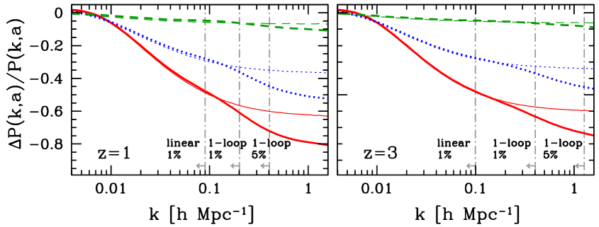
Perturbation theory is not expected to describe reality at very large k𝑘k values, since any perturbative expansion must break down when the evolution of structures becomes fully nonlinear. A good rule of thumb is to take as the valid regime the range of k𝑘k values at which the one-loop correction is smaller than the linear contribution [36]. More recent analyses show that for a ΛΛ\LambdaCDM cosmology, the one-loop corrected power spectrum deviates by less than 1% from N𝑁N-body simulation results provided that the dimensionless power spectrum, defined in this work as Δ2(k,τ)4πk3P(k,τ)superscriptΔ2𝑘𝜏4𝜋superscript𝑘3𝑃𝑘𝜏\Delta^{2}(k,\tau)\equiv 4\pi k^{3}P(k,\tau), does not exceed 0.4similar-toabsent0.4\sim 0.4 [37]. Applying this criterion to the total matter power spectrum in our ΛΛ\LambdaCHDM scenario, we expect our one-loop corrected power spectrum to be accurate to better than 1% for k < 0.2hMpc1𝑘 < 0.2superscriptMpc1k\mbox{\;\raisebox{1.29167pt}{$<$}$\!\!\!\!\!$\raisebox{-3.87495pt}{$\sim$}\;}0.2\ h\ {\rm Mpc}^{-1} at z=1𝑧1z=1 and k < 0.4hMpc1𝑘 < 0.4superscriptMpc1k\mbox{\;\raisebox{1.29167pt}{$<$}$\!\!\!\!\!$\raisebox{-3.87495pt}{$\sim$}\;}0.4\ h\ {\rm Mpc}^{-1} at z=3𝑧3z=3. For completeness we also estimate a 5% accurate region following figure 2 of [37]: k < 0.4hMpc1𝑘 < 0.4superscriptMpc1k\mbox{\;\raisebox{1.29167pt}{$<$}$\!\!\!\!\!$\raisebox{-3.87495pt}{$\sim$}\;}0.4\ h\ {\rm Mpc}^{-1} at z=1𝑧1z=1, and k < 1hMpc1𝑘 < 1superscriptMpc1k\mbox{\;\raisebox{1.29167pt}{$<$}$\!\!\!\!\!$\raisebox{-3.87495pt}{$\sim$}\;}1\ h\ {\rm Mpc}^{-1} at z=3𝑧3z=3.

It is also interesting to ask up to what values of k𝑘k is linear theory expected to provide an accurate description of the matter power spectrum. Comparing the total matter power spectrum computed from linear theory to that including the one-loop correction, we find 1% agreement between the two only at k < 0.09hMpc1𝑘 < 0.09superscriptMpc1k\mbox{\;\raisebox{1.29167pt}{$<$}$\!\!\!\!\!$\raisebox{-3.87495pt}{$\sim$}\;}0.09\ h\ {\rm Mpc}^{-1} for z=1𝑧1z=1 and k < 0.1hMpc1𝑘 < 0.1superscriptMpc1k\mbox{\;\raisebox{1.29167pt}{$<$}$\!\!\!\!\!$\raisebox{-3.87495pt}{$\sim$}\;}0.1\ h\ {\rm Mpc}^{-1} for z=3𝑧3z=3. From this we conclude that the one-loop correction improves on linear theory to better than 1% accuracy in the k𝑘k ranges

0.09 < k/(hMpc1) < 0.2,0.09 < 𝑘superscriptMpc1 < 0.2\displaystyle 0.09\mbox{\;\raisebox{1.29167pt}{$<$}$\!\!\!\!\!$\raisebox{-3.87495pt}{$\sim$}\;}k/(h\ {\rm Mpc}^{-1})\mbox{\;\raisebox{1.29167pt}{$<$}$\!\!\!\!\!$\raisebox{-3.87495pt}{$\sim$}\;}0.2, z=1,𝑧1\displaystyle z=1,
0.1 < k/(hMpc1) < 0.4,0.1 < 𝑘superscriptMpc1 < 0.4\displaystyle 0.1\mbox{\;\raisebox{1.29167pt}{$<$}$\!\!\!\!\!$\raisebox{-3.87495pt}{$\sim$}\;}k/(h\ {\rm Mpc}^{-1})\mbox{\;\raisebox{1.29167pt}{$<$}$\!\!\!\!\!$\raisebox{-3.87495pt}{$\sim$}\;}0.4, z=3.𝑧3\displaystyle z=3. (7.4a)

Figure 1 shows the various regions of validity discussed in this section.

8.3 Suppression due to neutrino free-streaming

Figure 2 shows the suppression in the total matter power spectrum due to neutrino hot dark matter for three ΛΛ\LambdaCHDM models with fν=0.1,0.05,0.01subscript𝑓𝜈0.10.050.01f_{\nu}=0.1,0.05,0.01, relative to the case with fν=0subscript𝑓𝜈0f_{\nu}=0, i.e.,

ΔP(k,a)P(k,a)Pfν0(k,a)Pfν=0(k,a)Pfν=0(k,a).Δ𝑃𝑘𝑎𝑃𝑘𝑎subscript𝑃subscript𝑓𝜈0𝑘𝑎subscript𝑃subscript𝑓𝜈0𝑘𝑎subscript𝑃subscript𝑓𝜈0𝑘𝑎\frac{\Delta P(k,a)}{P(k,a)}\equiv\frac{P_{f_{\nu}\neq 0}(k,a)-P_{f_{\nu}=0}(k,a)}{P_{f_{\nu}=0}(k,a)}. (7.4b)

Observe that the relative decrease of small scale power due to neutrino free-streaming in general exceeds the amount of suppression predicted by linear theory, once nonlinear corrections have been included. Within the 5% accurate region, it is clear that the suppression easily exceeds the canonical linear suppression factor of 8fνsimilar-toabsent8subscript𝑓𝜈\sim 8f_{\nu}.222The linear suppression factor reaches a maximum of 8fνsimilar-toabsent8subscript𝑓𝜈\sim 8f_{\nu} only for small values of fνsubscript𝑓𝜈f_{\nu}. For, e.g., fν=0.2subscript𝑓𝜈0.2f_{\nu}=0.2, the linear suppression factor is 4.5fνsimilar-toabsent4.5subscript𝑓𝜈\sim 4.5f_{\nu} [35]. This enhanced suppression has been observed in multi-component N𝑁N-body simulations [18], which support an asymptotic suppression factor of 9.8fνsimilar-toabsent9.8subscript𝑓𝜈\sim 9.8f_{\nu}. Furthermore, compared to the linear results, the one-loop correction leads to a small increase in relative power at just below k0.1hMpc1similar-to𝑘0.1superscriptMpc1k\sim 0.1\ h\ {\rm Mpc}^{-1}, before the enhanced suppression sets in, a feature that seems to be present also in figure 4 of [18]

A more rigorous comparison between our perturbation theory results and the N𝑁N-body results of [18] is not possible at present, since our results are valid only for z > 1𝑧 >1z\mbox{\;\raisebox{1.29167pt}{$>$}$\!\!\!\!\!$\raisebox{-3.87495pt}{$\sim$}}\;1, while reference [18] gives their results at z=0𝑧0z=0.

Refer to caption
Figure 2: Relative differences between the total matter power spectra for a pure ΛΛ\LambdaCDM cosmology and three ΛΛ\LambdaCHDM models with fν=0.1subscript𝑓𝜈0.1f_{\nu}=0.1 (red/solid), 0.05 (blue/dotted), and 0.01 (green/dash) at z=1𝑧1z=1 (left) and z=3𝑧3z=3 (right). Thick lines indicate results including the one-loop correction, while the linear results are represented by the thin lines. The three vertical lines indicate the maximum k𝑘k values at which the linear and the one-loop corrected matter power spectra are accurate to better than 1% and 5%.
Refer to caption
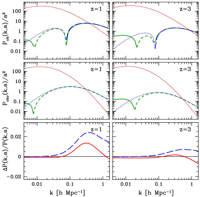
Figure 3: One-loop corrections to the CDM+baryon auto-correlation (top) and the CDM+baryon–neutrino cross-correlation (middle) at z=1𝑧1z=1 (left) and z=3𝑧3z=3 (right) for a ΛΛ\LambdaCHDM cosmology with fν=0.1subscript𝑓𝜈0.1f_{\nu}=0.1. In the top and middle rows, the red/thin solid lines indicate the linear contribution, while the green/thick solid lines denote the one-loop correction (green/short dash when negative). The blue/long dash lines represent an approximation to the one-loop correction (blue/dotted when negative), computed by setting S1,2,4=T1,,8=1subscript𝑆124subscript𝑇181S_{1,2,4}=T_{1,\cdots,8}=1 and S3=0subscript𝑆30S_{3}=0. The fractional error incurred in the total matter power spectrum by this approximation is shown in the bottom row in red/solid. Also plotted in the bottom row in blue/long dash is the fractional error incurred by neglecting the one-loop correction to the CDM+baryon–neutrino cross-correlation.

8.4 Further approximations?

There are two sources of deviation from the standard CDM-only case in the one-loop correction terms (7.1), (7.4h) and (7.4k). The first is encapsulated in the linear power spectra PcbL(k,τ)superscriptsubscript𝑃𝑐𝑏𝐿𝑘𝜏P_{cb}^{L}(k,\tau) and PcbνL(k,τ)superscriptsubscript𝑃𝑐𝑏𝜈𝐿𝑘𝜏P_{cb\nu}^{L}(k,\tau); the second in the factors S1,,4subscript𝑆14S_{1,\cdots,4} and T1,,8subscript𝑇18T_{1,\cdots,8} defined in equations (7.1) and (7.1), which depend on the linear growth functions. The linear power spectra are readily calculable with a sophisticated Boltzmann code such as CAMB. With some extra but minor effort the same is true also for the factors S1,,4subscript𝑆14S_{1,\cdots,4} and T1,,8subscript𝑇18T_{1,\cdots,8}. Nonetheless, it is tempting to simply assume S1,2,4=T1,,8=1subscript𝑆124subscript𝑇181S_{1,2,4}=T_{1,\cdots,8}=1 and S3=0subscript𝑆30S_{3}=0, as was done in [21]. In this section we examine the validity of this approximation.

Refer to caption
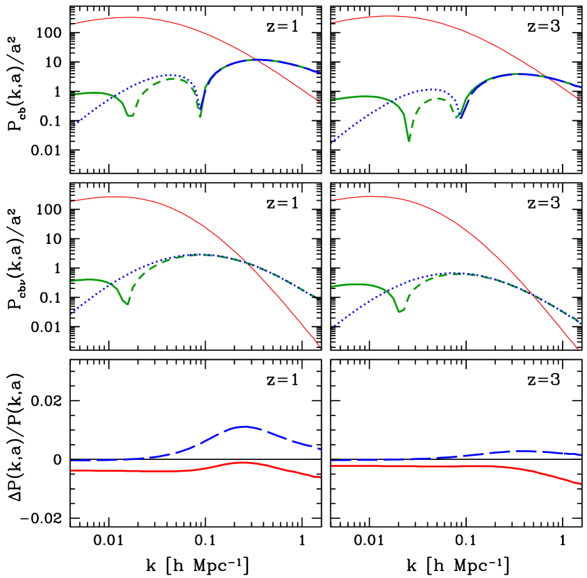
Figure 4: Same as figure 3, but for fν=0.05subscript𝑓𝜈0.05f_{\nu}=0.05.
Refer to caption
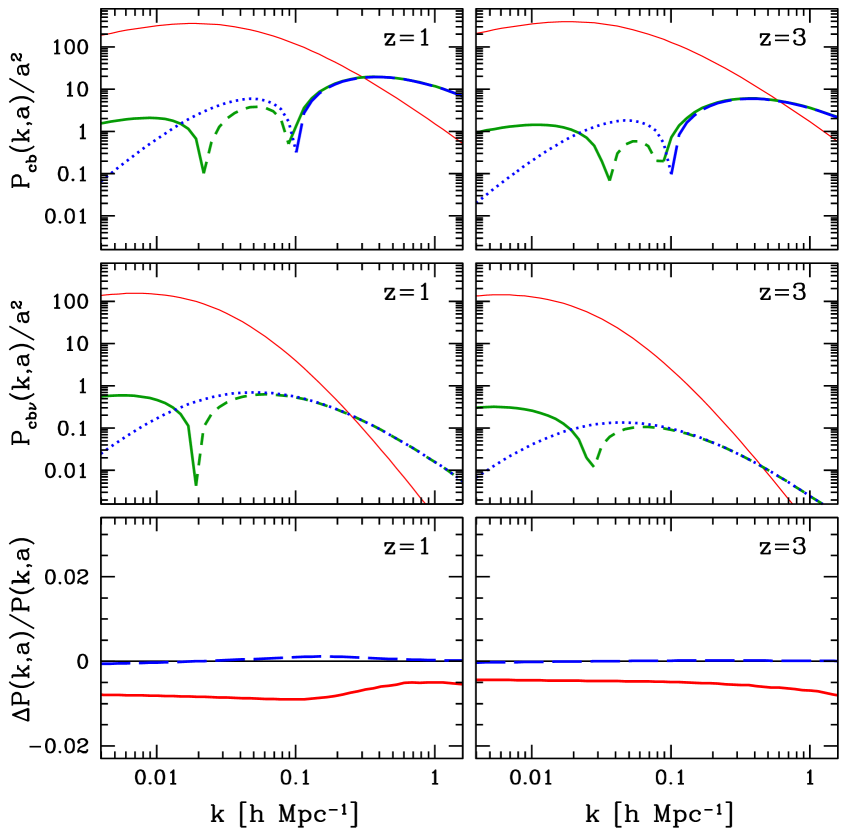
Figure 5: Same as figure 3, but for fν=0.01subscript𝑓𝜈0.01f_{\nu}=0.01.

Figures 3, 4 and 5 show the correction terms Pcb(22)+2Pcb(13)superscriptsubscript𝑃𝑐𝑏222superscriptsubscript𝑃𝑐𝑏13P_{cb}^{(22)}+2P_{cb}^{(13)} and Pcbν(13)superscriptsubscript𝑃𝑐𝑏𝜈13P_{cb\nu}^{(13)} computed under the assumption of S1,2,4=T1,,8=1subscript𝑆124subscript𝑇181S_{1,2,4}=T_{1,\cdots,8}=1 and S3=0subscript𝑆30S_{3}=0 for three ΛΛ\LambdaCHDM models with fν=0.1,0.05,0.01subscript𝑓𝜈0.10.050.01f_{\nu}=0.1,0.05,0.01 respectively. Compared with their correct forms, we find deviations as large as a factor of twenty, sometimes even accompanied by a sign flip. However, such large deviations are confined to a region at k0.1hMpc1much-less-than𝑘0.1superscriptMpc1k\ll 0.1\ h\ {\rm Mpc}^{-1}, where the one-loop correction terms are in any case subdominant to the linear contribution; the net fractional error incurred in the total matter power spectrum turns out to never exceed the 1% level for our choices of fνsubscript𝑓𝜈f_{\nu} and redshifts. Future cosmological probes will generally require an accuracy of 1similar-toabsent1\sim 1% in the matter power spectrum in order not to bias parameter estimation. On this basis, we conclude that setting S1,2,4=T1,,8=1subscript𝑆124subscript𝑇181S_{1,2,4}=T_{1,\cdots,8}=1 and S3=0subscript𝑆30S_{3}=0 is a tolerable simplification.

Also shown in figures 3, 4 and 5 are the consequences of dropping the Pcbν(13)(k,τ)superscriptsubscript𝑃𝑐𝑏𝜈13𝑘𝜏P_{cb\nu}^{(13)}(k,\tau) correction to the CDM+baryon–neutrino cross-correlation. As expected, the importance of this term increases as we increase fνsubscript𝑓𝜈f_{\nu}. For fν=0.1subscript𝑓𝜈0.1f_{\nu}=0.1, the maximum contribution of Pcbν(13)(k,τ)superscriptsubscript𝑃𝑐𝑏𝜈13𝑘𝜏P_{cb\nu}^{(13)}(k,\tau) to the z=1𝑧1z=1 total matter power spectrum is 2.5% at k0.4hMpc1similar-to𝑘0.4superscriptMpc1k\sim 0.4\ h\ {\rm Mpc}^{-1}. For fν=0.05subscript𝑓𝜈0.05f_{\nu}=0.05, the contribution is essentially halved. Thus for fν<0.05subscript𝑓𝜈0.05f_{\nu}<0.05, dropping the Pcbν(13)(k,τ)superscriptsubscript𝑃𝑐𝑏𝜈13𝑘𝜏P_{cb\nu}^{(13)}(k,\tau) term will unlikely bias our results. Nonetheless, Pcbν(13)(k,τ)superscriptsubscript𝑃𝑐𝑏𝜈13𝑘𝜏P_{cb\nu}^{(13)}(k,\tau) can be computed at essentially no extra expense to the user because of its similarity to the (mandatory) Pcb(13)(k,τ)superscriptsubscript𝑃𝑐𝑏13𝑘𝜏P_{cb}^{(13)}(k,\tau) contribution, cf. equation (7.4h). Hence there is no real need to resort to approximations in this instance.

9 Conclusions

In this paper we have presented the first rigorous and systematic derivation of the one-loop correction to the large scale matter power spectrum in a mixed dark matter cosmology with subdominant massive neutrino hot dark matter.

Beginning with the relevant equations of motion, we find that by invoking an “adiabatic” approximation, accurate to better than 0.1fνsimilar-toabsent0.1subscript𝑓𝜈\sim 0.1f_{\nu}, higher order corrections to the CDM+baryon density contrast and velocity field can be rendered into a form nearly identical to that for a pure-CDM cosmology. The interaction kernels and their recursion relations also exhibit striking similarities to their standard CDM-only counterparts, but contain additional dependences on the neutrino energy density fraction fνsubscript𝑓𝜈f_{\nu} and the linear growth functions of the incoming wavevectors. These results, generalised to n𝑛nth order in perturbative expansion, are summarised in equations (6) to (6).

Using these approximate solutions we compute the usual “22” and “13” one-loop correction terms to the matter power spectrum. As in the standard CDM-only case, these correction terms take the form of integrals over the wavevector 𝒒𝒒{\bm{q}} of the linear power spectrum PL(q,τ)superscript𝑃𝐿𝑞𝜏P^{L}(q,\tau) multiplied by the interaction kernels. In addition to the corrections to the CDM+baryon auto-correlation, we also find a one-loop correction term for the cross-correlation between the CDM+baryon and the neutrino components which was previously neglected. These correction terms appear in their evaluated and most simplified form in equations (7.1) to (7.4h), (7.4k) and (7.1).

Evaluating these expressions numerically, we find that nonlinear corrections to the large scale matter power spectrum can enhance the suppression of small scale power due to neutrino free-streaming relative to the fν=0subscript𝑓𝜈0f_{\nu}=0 case to beyond the canonical linear suppression factor of 8fνsimilar-toabsent8subscript𝑓𝜈\sim 8f_{\nu}. This enhanced suppression has been observed in multi-component N𝑁N-body simulations [18].

As said, the interaction kernels contain hitherto unaccounted dependences on fνsubscript𝑓𝜈f_{\nu} and the linear growth functions. Neglecting these dependences in principle generates large deviations in the one-loop corrections. However, since these deviations occur at wavenumbers at which the linear contribution dominates over the correction terms, their net effect on the total matter power spectrum never exceeds 1%. Future cosmological probes will require an accuracy of 1similar-toabsent1\sim 1% in the matter power spectrum in order not to bias parameter estimation. We have thus verified the validity of the approach of [21].

An important assumption in our present treatment is that the neutrino density perturbations have been taken to remain linear at all times. Although for realistic values of fνsubscript𝑓𝜈f_{\nu} this can be justified by N𝑁N-body simulation results [18], a truly complete analysis of higher order corrections to the clustering statistics of the large scale structure distribution in the presence of massive neutrinos should include also a proper account of nonlinear neutrino evolution. We defer this investigation to a future publication.

Finally, as noted in reference [21], although higher order perturbation theory appears at first glance to have a limited range of validity—we expect our one-loop corrections to improve on linear theory to better than 1% accuracy in the region 0.1 < k/(hMpc1) < 0.40.1 < 𝑘superscriptMpc1 < 0.40.1\mbox{\;\raisebox{1.29167pt}{$<$}$\!\!\!\!\!$\raisebox{-3.87495pt}{$\sim$}\;}k/(h\ {\rm Mpc}^{-1})\mbox{\;\raisebox{1.29167pt}{$<$}$\!\!\!\!\!$\raisebox{-3.87495pt}{$\sim$}\;}0.4 at z=3𝑧3z=3, it does enable an approximate factor of four increase in the maximum usable wavenumber in a data set. This is equivalent to a factor of 64 gain in the number of independent Fourier modes, or an eight-fold gain in statistical power for a fixed survey volume. Such an improvement is no small feat, and may very well be just what we need to detect neutrino dark matter.

Y3superscriptY3{\rm Y}^{3}W thanks Jacob Brandbyge, Steen Hannestad and Georg Raffelt for useful discussions and/or comments on the manuscript.
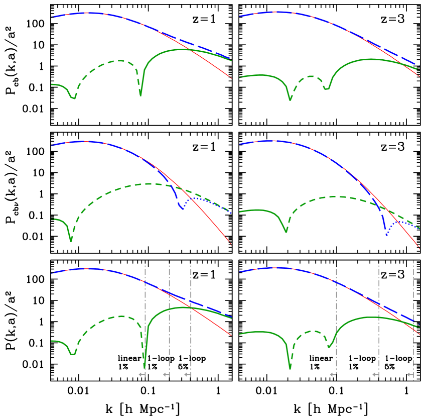
References

References

  • [1] C. Amsler et al. [Particle Data Group], “Review of particle physics,” Phys. Lett.  B 667 (2008) 1.
  • [2] J. R. Bond, G. Efstathiou and J. Silk, “Massive neutrinos and the large-scale structure of the universe,” Phys. Rev. Lett.  45 (1980) 1980.
  • [3] A. G. Doroshkevich, Y. B. Zeldovich, R. A. Sunyaev and M. Khlopov, “Astrophysical implications of the neutrino rest mass. II. The density-perturbation spectrum and small-scale fluctuations in the microwave background,” Sov. Astron. Lett.  6 (1980) 252 [Pisma Astron. Zh.  6 (1980) 457].
  • [4] A. G. Doroshkevich and M. Y. Khlopov, “The Development of Structure in a Neutrino Universe,” Sov. Astron. Lett.  25 (1981) 521.
  • [5] Q. Shafi and F. W. Stecker, “Implications Of A Class Of Grand Unified Theories For Large Scale Structure In The Universe,” Phys. Rev. Lett.  53 (1984) 1292.
  • [6] R. K. Schaefer, Q. Shafi and F. W. Stecker, “Large scale structure formation and cosmic microwave anisotropy in a cold plus hot dark matter universe,” Astrophys. J.  347 (1989) 575.
  • [7] J. Lesgourgues and S. Pastor, “Massive neutrinos and cosmology,” Phys. Rept.  429 (2006) 307 [arXiv:astro-ph/0603494].
  • [8] S. Hannestad, “Primordial neutrinos,” Ann. Rev. Nucl. Part. Sci.  56, 137 (2006) [arXiv:hep-ph/0602058].
  • [9] F. B. Abdalla and S. Rawlings, “Determining neutrino properties using future galaxy redshift surveys,” Mon. Not. Roy. Astron. Soc. 381 (2007) 1313 [arXiv:astro-ph/0702314].
  • [10] S. Hannestad and Y. Y. Y. Wong, “Neutrino mass from future high redshift galaxy surveys: Sensitivity and detection threshold,” JCAP 0707 (2007) 004 [arXiv:astro-ph/0703031].
  • [11] S. Hannestad, H. Tu and Y. Y. Y. Wong, “Measuring neutrino masses and dark energy with weak lensing tomography,” JCAP 0606 (2006) 025 [arXiv:astro-ph/0603019].
  • [12] T. D. Kitching, A. F. Heavens, L. Verde, P. Serra and A. Melchiorri, “Finding Evidence for Massive Neutrinos using 3D Weak Lensing,” Phys. Rev.  D 77 (2008) 103008 [arXiv:0801.4565 [astro-ph]].
  • [13] J. Lesgourgues, L. Perotto, S. Pastor and M. Piat, “Probing neutrino masses with CMB lensing extraction,” Phys. Rev.  D 73 (2006) 045021 [arXiv:astro-ph/0511735].
  • [14] S. Gratton, A. Lewis and G. Efstathiou, “Prospects for Constraining Neutrino Mass Using Planck and Lyman-Alpha Forest Data,” Phys. Rev.  D 77 (2008) 083507 [arXiv:0705.3100 [astro-ph]].
  • [15] K. Ichikawa and T. Takahashi, “On the determination of neutrino masses and dark energy evolution from the cross-correlation of CMB and LSS,” JCAP 0802 (2008) 017 [arXiv:astro-ph/0510849].
  • [16] J. Lesgourgues, W. Valkenburg and E. Gaztañaga, “Constraining neutrino masses with the ISW-galaxy correlation function,” Phys. Rev.  D 77 (2008) 063505 [arXiv:0710.5525 [astro-ph]].
  • [17] J. R. Pritchard and E. Pierpaoli, “Constraining massive neutrinos using cosmological 21 cm observations,” arXiv:0805.1920 [astro-ph].
  • [18] J. Brandbyge, S. Hannestad, T. Haugbølle and B. Thomsen, “The Effect of Thermal Neutrino Motion on the Non-linear Cosmological Matter Power Spectrum,” JCAP 0808 (2008) 020 [arXiv:0802.3700 [astro-ph]].
  • [19] K. Abazajian, E. R. Switzer, S. Dodelson, K. Heitmann and S. Habib, “The nonlinear cosmological matter power spectrum with massive neutrinos. I: The halo model,” Phys. Rev.  D 71 (2005) 043507 [arXiv:astro-ph/0411552].
  • [20] S. Hannestad, A. Ringwald, H. Tu and Y. Y. Y. Wong, “Is it possible to tell the difference between fermionic and bosonic hot dark matter?,” JCAP 0509 (2005) 014 [arXiv:astro-ph/0507544].
  • [21] S. Saito, M. Takada and A. Taruya, “Impact of massive neutrinos on nonlinear matter power spectrum,” Phys. Rev. Lett.  100 (2008) 191301 [arXiv:0801.0607 [astro-ph]].
  • [22] R. Juszkiewicz, “On the evolution of cosmological adiabatic perturbations in the weakly non-linear regime,” Mon. Not. Roy. Astron. Soc. 197 (1981) 931.
  • [23] E. T. Vishniac, “Why weakly non-linear effects are small in a zero-pressure cosmology,” Mon. Not. Roy. Astron. Soc. 203 (1983) 345.
  • [24] J. N. Fry, “The Galaxy correlation hierarchy in perturbation theory,” Astrophys. J.  279 (1984) 499.
  • [25] M. H. Goroff, B. Grinstein, S. J. Rey and M. B. Wise, “Coupling of Modes of Cosmological Mass Density Fluctuations,” Astrophys. J.  311 (1986) 6.
  • [26] F. Bernardeau, S. Colombi, E. Gaztañaga and R. Scoccimarro, “Large-scale structure of the universe and cosmological perturbation theory,” Phys. Rept.  367 (2002) 1 [arXiv:astro-ph/0112551].
  • [27] A. Ringwald and Y. Y. Y. Wong, “Gravitational clustering of relic neutrinos and implications for their detection,” JCAP 0412 (2004) 005 [arXiv:hep-ph/0408241].
  • [28] A. Lewis, A. Challinor and A. Lasenby, “Efficient Computation of CMB anisotropies in closed FRW models,” Astrophys. J.  538 (2000) 473 [arXiv:astro-ph/9911177].
  • [29] C. P. Ma and E. Bertschinger, “Cosmological perturbation theory in the synchronous and conformal Newtonian gauges,” Astrophys. J.  455 (1995) 7 [arXiv:astro-ph/9506072].
  • [30] W. Hu and D. J. Eisenstein, “Small scale perturbations in a general MDM cosmology,” Astrophys. J.  498 (1998) 497 [arXiv:astro-ph/9710216].
  • [31] J. N. Fry, “The Minimal power spectrum: Higher order contributions,” Astrophys. J.  421 (1994) 21.
  • [32] Y. Suto and M. Sasaki, “Quasi Nonlinear Theory Of Cosmological Selfgravitating Systems,” Phys. Rev. Lett.  66 (1991) 264.
  • [33] N. Makino, M. Sasaki and Y. Suto, “Analytic approach to the perturbative expansion of nonlinear gravitational fluctuations in cosmological density and velocity fields,” Phys. Rev.  D 46 (1992) 585.
  • [34] J. Dunkley et al. [WMAP Collaboration], “Five-Year Wilkinson Microwave Anisotropy Probe (WMAP) Observations: Likelihoods and Parameters from the WMAP data,” arXiv:0803.0586 [astro-ph].
  • [35] A. Kiakotou, Ø. Elgarøy and O. Lahav, “Neutrino Mass, Dark Energy, and the Linear Growth Factor,” Phys. Rev.  D 77 (2008) 063005 [arXiv:0709.0253 [astro-ph]].
  • [36] B. Jain and E. Bertschinger, “Second order power spectrum and nonlinear evolution at high redshift,” Astrophys. J.  431 (1994) 495 [arXiv:astro-ph/9311070].
  • [37] D. Jeong and E. Komatsu, “Perturbation Theory Reloaded: Analytical Calculation of Non-linearity in Baryonic Oscillations in the Real Space Matter Power Spectrum,” Astrophys. J.  651 (2006) 619 [arXiv:astro-ph/0604075].