Modeling of Body Mass Index by Newton’s Second Law

Abstract

Since laws of physics exist in nature, their possible relationship to terrestial growth is introduced. By considering the human body as a dynamic system of variable mass (and volume), growing under a gravity field, it is shown how natural laws may influence the vertical growth of humans. This approach makes sense because the non-linear percentile curves of different aspects of human physical growth from childhood to adolescence can be described in relation to physics laws independently of gender and nationality. Analytical relations for the dependence of stature, measured mass (weight), growth velocity (and their mix as the body mass index) on age are deduced with a set of common statistical parameters which could relate environmental, genetics and metabolism and different aspects of physical growth on earth. A relationship to the monotone smoothing using functional data analysis to estimate growth curves and its derivatives is established. A preliminary discussion is also presented on horizontal growth in an essentially weightless environment (i.e., aquatic) with a connection to the Laird-Gompertz formula for growth.

I Introduction

The raw (and theoretically smoothed) statistical data of different aspects of human physical growth from birth to adolescence have been collected for decades as a function of gender and nationality. From a practical point of view, these measurements are useful to monitor health care and to highlight secular trends on the fat intake (obesity) by a particular population Mor00 ; Qhe01 . Child growth records are also of special interest to Governments to enforce national health policies Fri90 .

In particular, there are smoothed growth charts for boys and girls such as those maintained by the USA National Center of Health Statistics (NCHS) nchs and the unsmoothed data for thousands of Japanese infants, children and adolescents (Hiroshima Growth Study Sample) Sumi . Typically, the charts consist of a set of non-linear percentile curves displaying the dependence on age of height $h(t)$, ”weight” $w(t)$ and combinations of them such as the weight-for-height and body mass index (BMI, i.e., ratio $B(t)\equiv w/h^{2}$). According to the CDC growth charts nchs , the $85^{th}$ percentile of BMI for children is considered the overweight threshold, and the $95^{th}$ percentile is the obesity threshold.

In constructing smoothed statistical growth curves a variety of asymptotic mathematical models have been tested to fit results for a population in retrospective Fle99 . Different trial functions are used because the data for $h$ and $w$ do not increase monotonically with age and because the use of weight-height methods (such as the BMI) affect directly the development of curve smoothing. For example, modeling of human anthropometric data has been done in the contexts of the lambda-mu-sigma (LMS) model Col90 , the model functions of triple logistic curves Boc76 , Count-Gompertz curves Kan90 ; Per02 and Jolicoeur et al. curves Jol92 . Another fine test model used is the infancy-childhood-puberty (ICP) model Kar89 . This model breaks down growth mathematically into different (exponential, quadratic and logistic) functions using different curve fitting procedures out of the growth data. Predictions of changes in height have also been carried out according to an empirical Bayesian approach Sho91 . The selection of a definitive parametric approach for the inclusion or exclusion of some empirical data points and to set a criteria of estimation is a topic of active discussions because of its relevance to growth, development and aging in living organisms Fle99 .

For open systems like those in which there are influx of mass, one can apply the conservation of linear momentum and energy methods of general physics to study their growth dynamics. Examples in which momentum is gained from, or lost to, the surroundings include rockets Hal78 ; Sou02 and the falling of a snow ball Dia03 , respectively. Since the human body is also a system of fluctuating mass (and volume), under the influences of the acceleration of gravity $g$ and food consumption, it is not unreasonable to consider it as a dynamic physics system. One may then in principle make an attempt to derive a relationship based on physics laws and observed ”physical” growth.

Since laws of physics exist in nature, their possible relationship to human physical growth is introduced in this work. It is shown how physics seems to influence the physical growth of humans. Using Newton’s second law, analytical relations are deduced for the time dependence of $h$, $w$, the growth velocity $v=dh/dt$ which depend on common parameters that could relate other aspects of this phenomenon such as environmental conditions and genetics and natural processes like metabolism, energy supplied by food, etc. Within a simple physics-based framework, estimates of all observed human growth statistical data including BMI on age are easily performed and are shown to fit the observed data which makes the present model reasonable. A preliminary discussion on horizontal growth in an essentially weightless environment is also presented with a connection to the Laird-Gompertz formula for aquatic growth.

II Simple Physics Characterization

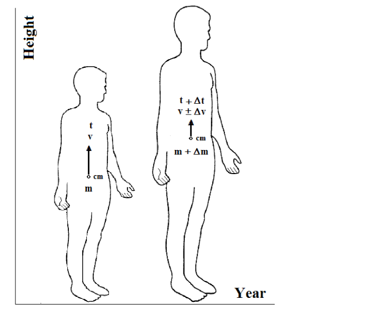
Let us consider the human body as a system of variable mass $m(t)$, where mass is the amount of matter present in the body measured using balance. In Fig.1 the approximated center of mass of an upright body as seen from a particular reference frame at different ages is illustrated. In scientific usage mass is an intrinsic property of matter and weight is a force that results from the action of gravity on matter. In everyday usage, however, weight and mass are used interchangeably. The reported ”weight” in the smoothed growth charts for humans in nchs ; Sumi corresponds to measured matter or mass in kilograms and not to the force of weight ”$w(t)=m(t)g$” measured in Newtons. In the following such ”weight” data is referred as measured mass for the sake of correctness. Changes of mass and momentum will be assumed to be continuous during the growing process through years from childhood to maturity.

To derive the equation of motion of the body system whose mass is not constant, let us use Newton’s second law to define the external force $F$ on the human body. As shown explicitly in Appendix A, this is expressed as (see, e.g., Hal78 )

$$m\;\frac{d{\bf v}}{dt}={\bf F}_{\it ext}+{\bf v}_{\it rel}\;\frac{dm}{dt}\;\;\;,$$ (1)

where $dm/dt>0$ is the rate at which mass is gain (i.e., equivalent to particles entering an open system) and ${\bf v}_{\it rel}(t)$ is the relative velocity of the gained mass with respect to the body moving with a growth velocity of magnitude $v(t)\equiv|{\bf v}(t)|$. The above term $\phi(t)\equiv{\bf v}_{\it rel}\;(dm/dt)$ corresponds to the momentum flux being tranferred into the body by the added mass. This is interpreted as the force exerted on the body by the mass that joins it Sou02 and ${\bf F}_{ext}$ is the external force of gravity acting on the variable mass system. The surface of the earth is taken as the zero level of gravitational potential energy.

In applying the Newton law for the vertical growth of humans, it corresponds to the analysis of an extended system of $N$ particles rather than to the analysis of a single particle of mass $m_{i}$ and velocity ${\bf v}_{i}$ at time $t$. In this case one can only consider averaged values for all the physical quantities -such as the external force, due to the complexity of the body system. Hence, if $n(h_{i})$ is the number of objects at various heights $h_{i}$, of a total of $n$ objects distributed among $\ell$ heigths, then the mean average value of any given function $f$ for those objects is in general

$$\hat{f}\equiv<f_{i}>=\frac{1}{n}\sum_{i=1}^{\ell}n(h_{i})\;f_{i}=\sum_{i=1}^{\ell}\frac{n(h_{i})}{n}\;f_{i}=\sum_{i=1}^{\ell}\rho_{i}\;f_{i}\;\;\;,$$ (2)

where $\rho_{i}$ is interpreted as the probability that a fraction of the objects $n(h_{i})/n$ has the height $h_{i}$. So as the sum of all fractions of the whole system is unity ($f=1$), the probability distribution function is also normalized such that $\sum_{i=1}^{\ell}\rho_{i}=1$. It can be seen that $\rho_{i}$ directly affect the outcome of averaged results since it weights the values of the given function $f$ at each height $i$. The above mean value equation is used throughout the theory of statistical physics.

Let us consider next the number of $n$ objects distributed among $\ell$ heights as being $N$ sets or groups of particles of added mass $m_{i}$ each at time $t$. Then the mean value for the external force of Eq.(1) in one longitudinal direction becomes

$$\hat{F}_{\it ext}\equiv<F_{i,\it ext}>=\sum_{i}^{N}\rho_{i}\left\{m_{i}\;\frac{dv_{i}}{dt}-v_{i,\it rel}\;\frac{dm_{i}}{dt}\right\}\;\;\;.$$ (3)

Statistically stationary states in which all the probabilities $\rho$ are time independent $\forall i$ will be only considered.

To an observer at rest on the earth, the accumulating particles in the body at a given time appear to move at a velocity, say $v_{a}(t)$, proportional to the growth velocity $v(t)$ of the center of mass. For simplicity let us consider an homogenous system so that such a proportionality is set equal to one, i.e. $v_{a}(t)\approx v(t)$, which corresponds to the maximum velocity that the added mass alone can achieve during the grow. This is so because the human growth in stature is longitudinal until reaching a maximum height $h(\infty)$ with respect to earth’s surface (and a maximum mass $m(\infty)$ under healthy conditions) at adolescence (see Fig.1). On the other hand, to an observer on the center of mass of the body, the added mass appears to have a vertical motion with a velocity of magnitude $v(t)+v_{a}(t)\approx 2v(t)$ in the opposite direction of the growth with respect to the center of mass displacements. Therefore, for the present purposes, the relative velocity ${\bf v}_{\it rel}(t)$ of the gained mass appears to move at twice the velocity of growth as seen from within the body system, namely $|{\bf v}_{\it rel}|=2|{\bf v}|$. Hence Eq.(3) for the mean value of the net external force on the body as a whole is the superposition of contributions

$$\hat{F}_{\it ext}(t)=<F_{i,ext}(t)>=\sum_{i=1}^{N}\rho_{i}\;m_{i}(t)\;\frac{dv_{i}(t)}{dt}-2\sum_{i=1}^{N}\rho_{i}\;v_{i}(t)\;\frac{dm_{i}(t)}{dt}\;\;\;.$$ (4)

with $\rho$ the normalized probability distribution function of $N$ objects or set of particles of added mass $m_{i}$ each at time $t$.

The force of gravity $F_{g}$ due to the earth mass acting thoughout the human body must be also taken into account. Similarly to suspended chains systems Sou02 , this force is not only proportional to the total weight of the body at an given height $h(t)$, but also to the total force due to the amount of mass at rest lying on the surface of the earth. This extra term can also be understood by the fact that the volume (besides the mass) of the human body also varies. It accounts for an additional momentum that the system acquires as a result of changing volume (in one-dimension vertical) with years –see Appendix A. In this case, the force of gravity acting on the $N$ objects of added mass $m_{i}$ is then given by

$$\hat{F}_{g}(t)=\sum_{i=1}^{N}\left\{\rho_{i}\;\frac{h_{i}(t)}{h_{i}(\infty)}m_{i}(t)\right\}g-w(\infty)=<\lambda_{i}(t)h_{i}(t)>g-m(\infty)g\;\;\;,$$ (5)

where $\lambda_{i}(t)\equiv m_{i}(t)/h_{i}(\infty)$ represents mass per unit height. The weight at rest term $w(\infty)=m(\infty)g=<m_{i}(\infty)>g=\sum_{i=1}^{N}\rho_{i}m_{i}(\infty)g$ is deduced according to the boundary condition $\hat{F}_{g}\rightarrow 0$ as $t\rightarrow\infty$.

III General Biometric formulae

In order to derive analytical relations for the dependence of stature, measured mass (weight), growth velocity (and their mix as the body mass index) on age, let us proceed by considering Newton’s law of motion in relation to the two distinct mean forces acting on the system, i.e. the net external force of Eq.(4) and the gravity force of Eq.(5). This means to set $\hat{F}_{g}=\hat{F}_{\it ext}$, or more explicitly

$$\sum_{i=1}^{N}\rho_{i}\left\{m_{i}(t)\;\frac{dh^{2}_{i}(t)}{dt^{2}}-2\left(\frac{dh_{i}(t)}{dt}\right)\left(\frac{dm_{i}(t)}{dt}\right)-\frac{h_{i}(t)}{h_{i}(\infty)}\;m_{i}(t)g\right\}=-m(\infty)\;g\;\;\;,$$ (6)

with $v_{i}(t)=dh_{i}(t)/dt$. After some little algebra, and using the well-known trigonometric relation: $sech^{2}+tanh^{2}=1$, it is straightforward to check that this second order differential equation has the general solutions

$$h(t)=<h_{i}(t)>=\sum_{i=1}^{N}\rho_{i}h_{i}(\infty)\;tanh\left(\frac{t-t_{i}}{\tau_{i}}\right)\;\;\;,$$ (7)

such that

$$h_{i}(\infty)=\frac{1}{2}g\tau_{i}^{2}\;\;\;,$$ (8)

with $t_{i}$, and $\tau_{i}$ time lags for $i$ sets of particles. The mean value of $\tau_{i}$ is deduced by considering the limit $t\rightarrow\infty$, which leads to $h(\infty)=<h_{i}(\infty)>=\sum_{i=1}^{N}\rho_{i}h_{i}(\infty)=g<\tau_{i}^{2}>/2$. In this way, the mean time lag $<\tau_{i}>$ is interpreted as the time at which the growth velocity becomes zero and the maximun body height is achieved with respect to the earth’s surface $h(0)=0$ (recall that $x(t)=x(0)+v(t)*t+\frac{1}{2}a(t)*t^{2}$ from Newton’s mechanics for constant mass systems). On the other hand, $t_{i}$ are the time lags at which the single height contributions $h_{i}(t)$ of the $N$ objects or set of particles become zero.

Furthermore,

$$v(t)=\frac{dh(t)}{dt}=<\frac{dh_{i}(t)}{dt}>=\sum_{i=1}^{N}\rho_{i}\frac{h_{i}(\infty)}{\tau_{i}}\;sech^{2}\left(\frac{t-t_{i}}{\tau_{i}}\right)\;\;\;,$$ (9)

which for $t\rightarrow\infty$, it gives $v(\infty)\rightarrow 0$ as expected (after completion of the physical growth), and

$$m(t)=<m_{i}(t)>=\sum_{i=1}^{N}\rho_{i}m_{i}(\infty)\;tanh\left(\frac{t-t_{i}}{\tau_{i}}\right)\;\;\;.$$ (10)

It follows inmediately that physics theory predicts that the height and mass functions reach maximum values (plateau) on age due to the presence of the hyperbolic tangent functions. The mass per unit height $\lambda_{i}(\infty)=m_{i}(\infty)/h_{i}(\infty)\neq 0$ corresponds to the slope of $m_{i}(t)$ versus $h_{i}(t)$. For systems of variable mass, the center of mass velocity $v(t)$ is not the same as that for the $N$ sets of particles in the system $v_{i}$. In turn, the moving particles may not have the same velocities for each state $i$.

IV Physics estimates of human growth data

To this point, the amount of growth parameters in the present physics based biometric formulae seems to be large. However, these are not only comparable with those in the alternative asymptotic mathematical models tested for the modeling of human anthropometric data (see, e.g., Fle99 ; Col90 ; Boc76 ; Kan90 ; Per02 ; Jol92 ; Kar89 ; Sho91 ), but their number can still be reduced –at least for small $N$ sets of particles.

It is easy to verify by a plot that for $y\geq 0$, the monotonicity of the hyperbolic tangent implies the relation Mali01

$$tanh\;y\;\leq 1\leq\frac{tanh\;(xy)}{tanh\;x}\;\;\;.$$ (11)

Therefore, using this inequality it is possible to group together model parameters to set lower bounds to all functions in this work. In fact, by setting $y=\tau/\tau_{i}\rightarrow 1/\epsilon_{i}\geq 0$ (independent of $t$) and $x\rightarrow(t-t_{i})/\tau$, such that $\tau_{i}\equiv\epsilon_{i}\tau$, one obtains

$$tanh\;(xy)=tanh\;\left(\left[\frac{t-t_{i}}{\tau}\right]\;\left[\frac{\tau}{\tau_{i}}\right]\right)\geq tanh\;\left(\frac{\tau}{\tau_{i}}\right)tanh\;\left(\frac{t-t_{i}}{\tau}\right)=tanh\;y\;tanh\;x\;\;\;.$$ (12)

Hence Eqs.(7) and (10) can be approximated as

$$h(t)\geq\sum_{i=1}^{N}A_{i}\;tanh\left(\frac{t-t_{i}}{\tau}\right)\;\;\;.$$ (13)

and

$$m(t)\geq\sum_{i=1}^{N}B_{i}\;tanh\left(\frac{t-t_{i}}{\tau}\right)\;\;\;,$$ (14)

where, $\forall i$, it is defined

$$A_{i}\equiv\rho_{i}h_{i}(\infty)\;tanh\left(\frac{1}{\epsilon_{i}}\right)=\rho_{i}h_{i}(\infty)\;tanh\left(\frac{\tau}{\tau_{i}}\right)\;\;\;,\;\;\;B_{i}\equiv\lambda_{i}(\infty)A_{i}\;\;\;,$$ (15)

with $\lambda$ is mass per unit height as before. Since the $\tau_{i}$ parameters are related to $h_{i}$ via the Newtown equation in Eq.(8), then this leads to the positive dimesionless quantities $\epsilon_{i}=(1/\tau)\sqrt{2h_{i}(\infty)/g}$. Furthermore, the momentum flux tranferred to the body by the added $m_{i}$ becomes $\phi_{i}(t)\equiv v_{i}\;(dm_{i}/dt)=(B_{i}/A_{i})\;v_{i}(t)^{2}$, similarly to nonrigid systems Sou02 .

Taking the derivative of Eq.(13) it follows that

$$v(t)\geq\frac{1}{\tau}\sum_{i=1}^{N}A_{i}\;sech^{2}\left(\frac{t-t_{i}}{\tau}\right)\;\;\;.$$ (16)

which is consistent with Eq.(9) in the lower bound since $(1/\tau_{i})sech^{2}(xy)\geq(1/\tau)\;tanh\;y\;sech^{2}\;x$.

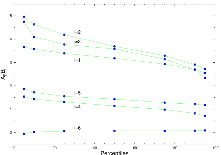
In this way, the unkown growth parameters $h_{i}(\infty)$, $m_{i}(\infty)$ and $\rho_{i}$ can reduce to $A_{i}$ and $B_{i}$, which will be referred to as ”biological parameters”. Together with the time lag $\tau$ and the peak positions of each $tanh$ function, given by $t_{i}$, these parameters allow to describe non-linear percentile curves (or alternatively z-scores Fle99 ) as shown next.

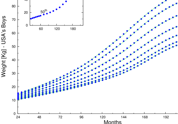
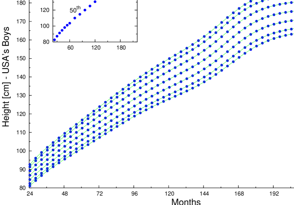
Selected smoothed empirical percentiles of measured mass (weight)- and height-for-age from the boys data based on medical literature nchs are shown in Figs 2 and 3 by dots, respectively. The theoretical curves (full lines) are obtained using Eqs.(14) and (13) assuming $N=6$ sets of particles with the biological parameters $A_{i}/B_{i}$ of Eq.(15) illustrated in Fig.4. All parameter values can easily be derived using the fit command of the free GNUPlot data plotting software. Real (smoothed and unsmoothed) data curves for boys and girls increase monotonically with age independent of gender and race Fle99 ; Col90 ; Boc76 ; Kan90 ; Per02 ; Jol92 ; Kar89 ; Sho91 . In the inserts, unsmoothed $50\%$ percentile empirical points for $w(t)$ and $h(t)$ of Chinese girls ages 6-18 years Chan65 are shown for comparison to display observed characteristic trends.

In order to show that there is not need for guessing some mathematical functions a priori, let us fit the smoothed curves rather than the raw data. A similar behaviour to the reported smoothed curves is obtained from the Newton dynamics of systems with variable $m$. Within measurements error, the variation of estimates of growth charts is close to all smoothed empirical data in the figures (usually measured to the nearest $0.1cm$ Xxu02 ). Both the height-for-age and measured mass-for-age tend to a maximum. According to these results, it can be argued that for each plotted point, the variable mass and height (and growth velocity as seen below) of humans can be correlated in relation to physics laws over many years.

At the origin, the boundary conditions $h(0)=0$ and $m(0)=0$ in Eqs.(13) and (14) lead to the relations between the biological parameters

$$A_{1}\;tanh\left(\frac{t_{1}}{\tau}\right)\leq\sum_{i=2}^{N}A_{i}\;tanh\left(\frac{t_{i}}{\tau}\right)\;\;\;;\;\;\;B_{1}\;tanh\left(\frac{t_{1}}{\tau}\right)\leq\sum_{i=2}^{N}B_{i}\;tanh\left(\frac{t_{i}}{\tau}\right)\;\;\;,$$ (17)

where $t_{1}<0$ and $t_{2},\cdots,t_{N}>0$ which leads to reduce further the number of parameter values. In fact, as $t\rightarrow\infty$, $tanh\;t_{{}_{i\;>N}}\rightarrow 1$ and $B_{{}_{i\;>N}}\rightarrow 0$ for finite $N$ sets of particles (of added matter $m_{{}_{i\;\leq N}}$).

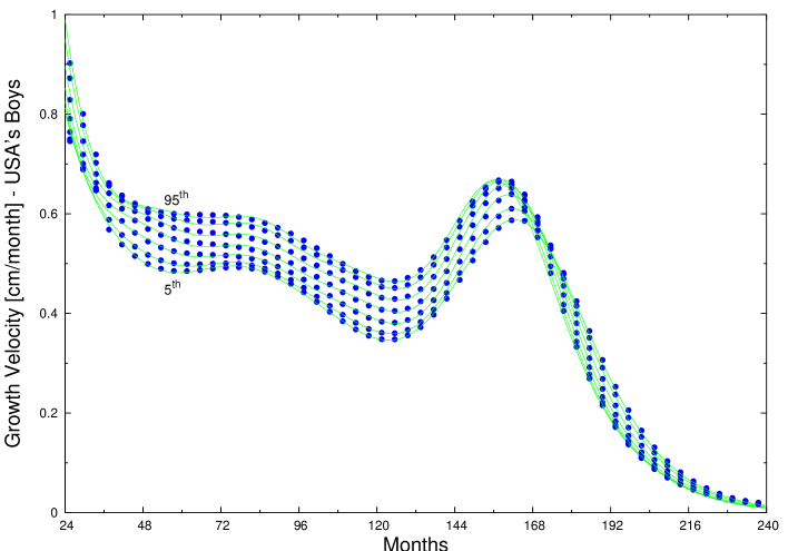
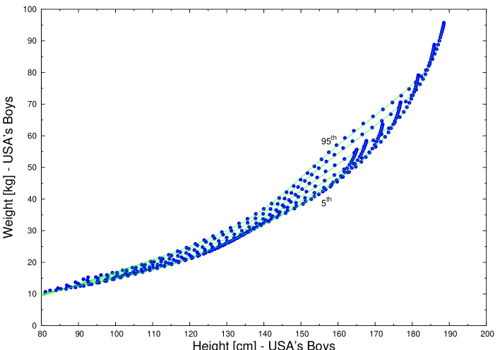
In humans growth is a natural process characterized by periods of growth spurts during early infancy and again at puberty. In Figs.5 and 6 illustrated by dots are the growth velocity curves and the measured mass (weight)-for-height curves at different percentiles, respectively nchs . The full lines in these figures correspond to results obtained from Eq.(16) and Eqs.(14)-(13), using parameters as before. As shown in Fig.5, the growth velocity oscillates down as a function of time to vanish in the adolescence. The system acceleration $dv/dt$ changes sign over the years due to the $tanh$ term in the derivative of Eq.(16). On the other hand, both the real and the mass-for-height model curves of Fig.6 increase monotonically. The $5^{th}$ percentile in this case is considered as an underweight threshold nchs . Such weight-for-height standards are used in the study of nutrition status and mortality risk in a community Fri90 .

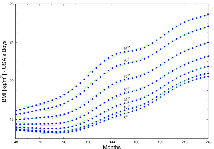
Further evidence for a relation between physics laws and human growth is given by looking at the BMI on age plotted in Fig.7 for selected percentiles. On equal grounds, the plotted dots are evaluations using the measured mass and heigth on age using the smoothed charts of Figs.2 and 3 nchs and the full line curves from $m(t)/h(t)^{2}=<m_{i}(t)>/<h_{i}(t)>^{2}$ with the biological parameters in Fig.4. It can be seen that the present estimates of BMI are reasonably close to the reported smoothed data. BMI fluctuations increase with the error of the data for $h^{2}$. This is reflected in BMI calculations for younger ages at the higher percentiles. Theoretical BMI curves at the lower percentiles display a minima with increasing age from 3 to about 6 years to then rise steadily with age as observed in reality. Within the physics approach, this minimium is a consequence of the growth spurts at early infancy depicted in Fig.5. Increasing $N$ in the sums of Eqs.(14) and (13) allows a better minima fit at higher percentiles of the BMI-for-age curves.

V Remarks

The present study is not based on arbitrary mathematical trial functions to fit the human physical growth data. All general trends for the observed non-linear percentile curves displaying the distribution of different aspects of human physical growth from childhood to adolescence have been understood and described in relation to physics laws that are daily perceived by living on the surface of the earth.

As shown here theoretically (see Appendix A for details on the derivation of the general Newton approach in question), the underlying physics of Newtonian mechanics is the bases of the derivation of all equations. The coefficients at each stage of the derivations are the consequence of dealing with the differential equation (1) applied to a very dense data set based on human growth. This also include the fundamental function, $tanh(x)$ appearing throughout the resulting relations for the body height in Eq.(7) , mass in Eq.(10) and BMI thereafter. Therefore $tanh(x)$ here is not made arbitrarily to fit a wide range of data from a set of adjustable, weighted coefficients. On the other hand, the peaked growth velocity of Eq.(9) depends on the different hyperbolic function $sech(x)$.

Alternative models to estimate growth curves and their derivates, such as the growth velocity, are based on the use of a non-parametric monotone smoothing process of the form Ram02

$$\mu(t)=\beta_{0}+\beta_{1}\int_{0}^{t}exp\{W(u)\}du\;\;\;.$$ (18)

The regression coefficients $\beta_{0,1}$ set the origin and range required to fit $\mu$ data including the velocity curves $v(t)$ on age to account for the pubertal growth spurt. The $\mu(t)\rightarrow v(t)$ function is constructed using the functional data object $W(u)$ which does not approximate the measured data directly, but rather after some exponential transformations (to make $\mu$ positive) and integration up to $t$ (to make $\mu$ increasing or monotonic). A relationship between the present physics based approach and the monotone smoothing can be established as shown explicitly in Appendix B.

The tendency to predict and describe growth by normal curves often obscures individual growth spurt phases that are consistently present but asynchronous across the population as a whole Ram02 . To this end, one can deduce that since the present growth theory is based on the law of gravity which influences individuals, then either a single contribution, or the superposition of contributions, on the growth curves are driven by the same general patterns described as derived by Newton’s law in Eq.(1).

When dealing with an extended system such as the human body, Newton’s second law states that the net external force applied to the center of mass equals the center of mass acceleration times the mass, namely ${\bf F}_{\it ext}=M{\bf a}_{\it(cm)}$. According to Eq.(4) one can then write $\hat{F}_{\it ext}=<m_{i}v_{i}\;(dv_{i}/dh_{i})-2v_{i}^{2}\;(dm_{i}/dh_{i})>=<m_{i}(\infty)a_{i\it(cm)}>$. Using the average definition in Eq.(2), e.g.,$m=<m_{i}>$, in conjuction with the definiton of mass-per-unit height $\lambda_{i}(\infty)\equiv m_{i}(\infty)/h_{i}(\infty)$ and Eqs.(13)-(15) it follows that $h_{i}(t)=(h_{i}(\infty)/m_{i}(\infty))m_{i}(t)$ and $v_{i}(t)=h_{i}(\infty)(dm_{i}(t)/dt)$. Hence $h_{i}(\infty)a_{i\it(cm)}\equiv h_{i}\;(dv_{i}/dt)-2\;v_{i}^{2}$. The latter corresponds to the difference between the center of mass acceleration of a uniform rod of height $L$ lifted with a variable velocity $v$, namely $L\times a_{\it(cm)}^{\it rod}=v^{2}+x\;(dv/dt)$, and that of a uniform rod of height $L^{\prime}=L/3$ lifted with constant velocity $v^{\prime}=v$, namely $L^{\prime}\times a_{\it(cm)}^{\it rod^{\prime}}=v^{\prime 2}$. This superposition may reflect the fact that the center of mass of the human body –whose mass distribution can also change by pelvic rotation and displacement, knee flexion, foot mechanisms– has not a fixed location on time Ore04 . There are alternative models based on Newton mechanics to study mass redistribution throughout the body as a function of age and applied forces (see, i.e., Jen89 ). By applying the equation of motion for the human body with variable mass as discussed here, it could be helpful to understand the extent to which empirical models by inverse dynamics to derive the torque (moment) correspond to prediction as well as their affect on human movement.

The primarily interest in human physical growth and its relationship to physics laws is to enhance the fit quality to observed data and to understand the underlying phenomena. There is overwhelming biological evidence that continuous growth processes on earth proceed by multiplicative increments, therefore the body size of plants, animals and humans follows a lognormal rather a normal distribution (with additive increments) Hux32 . Thus one should not expect human height distributions to be normal but lognormal Sch02 . The claim here is not modified by either class of $\rho_{i}$ distributions –relating the biological parameters in Eq.(15). In principle, one may associate these parameters to changes in kinetic energy of the center of mass of the system Sou02 , and the thermal internal energy, via the integral of $\hat{F}_{\it ext}(t)$ in Eq.(4) with respect to $x_{\it(cm)}^{rod}=x^{2}/2L-x^{\prime 2}/2L^{\prime}$.

The relationship between natural laws and human physical growth as introduced in this work may be also suitable to understand the biometrics of other living species growing vertically such as Primates Lei01 (and perhaps leaving trees and plants too). However, at this point, it is also worth to ask if the same physics laws discussed here can also be applied in the case of horizontally growing terrestial organisms, i.e., those organisms growing in an essentially weightless environment (aquatic organisms as white-side Dolphins Fer96 ).

So the question is: Can horizontal growth be also described within the present physics approach in the ”absence” of gravity ($g\rightarrow 0$) as contrary to vertical growth where gravity influences directly?

Let us attempt to reply this crucial question and see how the present model may provide a unique description for both cases. Consider the general Eq.(4) for $\hat{F}_{\it ext}$ again and set the force of gravity equal to $\hat{F}_{g}=0$. Alternatively, from Eq.(5) this implies $h_{i}(t)\rightarrow h_{i}(\infty)=const.$ which means to compensate out the weight $w(t)$ with the volume dependent forces. Therefore

$$\sum_{i=1}^{N}\rho_{i}\;m_{i}(t)\;\frac{dv_{i}(t)}{dt}-2\sum_{i=1}^{N}\rho_{i}\;v_{i}(t)\;\frac{dm_{i}(t)}{dt}=0\;\;\;.$$ (19)

One solution satisfies

$$m_{i}(t)\;\frac{dv_{i}(t)}{dt}=\;2v_{i}(t)\;\frac{dm_{i}(t)}{dt}\;\;\;,$$ (20)

or

$$\frac{dv_{i}(t)}{v_{i}(t)}=2\;\frac{dm_{i}(t)}{m_{i}(t)}\;\;\;,$$ (21)

which, by integration, implies the relation

$$v_{i}(t)\equiv\frac{dx_{i}(t)}{dt}=\gamma m_{i}^{2}(t)\;\;\;,$$ (22)

or

$$v(t)=<v_{i}(t)>=\gamma<m_{i}^{2}(t)>\;\;\;,$$ (23)

with $\gamma$ a constant for a given aquatic specie and for the long $x$-axis of a horizontal structure.

On the other hand, let us consider (and expand in Taylor series) the well-known Laird-Gompertz empirical formula for fish growth Fer96 ; Reg80 . That is

$$\frac{x(t)}{x_{0}} = e^{a\;(1-e^{-\alpha t})}$$ (24)

$$\approx 1+a\;(1-e^{-\alpha t})$$

$$= 1+a\;\left(1-\frac{1}{e^{\alpha t}}\right)$$

$$\approx 1+a\;\left(1-\frac{1}{1+\alpha t}\right)\;\;\;$$

where $x(t)$ is the lenght at age $t$ (at zero gravity) and $(a,\alpha)$ are specific rates of the exponential growth. It follows that the growth velocity $v(t)\equiv dx(t)/dt$ satisfies

$$v(t)=\frac{ax_{0}\alpha}{(1+\alpha t)^{2}}=\frac{\alpha}{ax_{0}}[(1+a)x_{0}-x(t)]^{2}\;\;\;.$$ (25)

Using the Chebyshev’s sum inequality $\sum_{k=1}^{n}a_{k}b_{k}\geq(1/n)\sum_{k=1}^{n}a_{k}\sum_{k=1}^{n}b_{k}$, such that $a_{k}=b_{k}=\rho_{i}m_{i}\equiv\rho m_{i}$, then comparison of Eqs.(22) and (25) results in $<m_{i}(t)>^{2}\;\leq N\rho\sum_{i=1}^{N}\rho m_{i}(t)^{2}=N\rho<m_{i}^{2}(t)>$ and

$$m(t)\leq\left(\frac{N\rho\alpha}{ax_{0}\gamma}\right)^{1/2}|(1+a)x_{0}-x(t)|\;\;\;.$$ (26)

which for values $x(t)>(1+a)x_{0}$, it implies an approximated linear relation between mass and length for horizontal growth (the mass-for-height for vertical growth under the influence of gravity is plotted in Fig.6 for comparison).

To this end, collected data reported in Fer96 for white-side Dolphins in the central north pacific ocean suggest that the postnatal dentine thinkness of Dolphins (used as an index of age in these animals) increases linearly with the total body length. It is reasonable to then justify the linear proportion between the aquatic species mass and length of the type in Eq.(26), as a consequence of the application of physical laws (c.f., Eq.(4)), in conjuction with the Laird-Gompertz growth function (c.f., Eq.(24)). Relations (24) and (26) also allows to study the BMI for aquatic organisms and Eq.(25) to predict their growth velocity curves in terms of the square of their mass (c.f., Eq.(23)).

Therefore, the absence of gravitational forces during growth in secondarily aquatic tetrapods (SAT) –backboned, limbed, air-breathing animals with ancestors that evolved in a terrestrial environment where gravity was a factor in growth and motion (e.g., Dolphins)– leads to mass and body length trajectories that, in principle, could be replicated by the present general physics model. Further multidisciplinary research along these lines is needed to shed new light on the fundamentals of growth in all classes of terrestrial organisms using one model based on Newton’s second law as discussed here.

APPENDIX A

Let us follow Refs. Hal78 ; Sou02 to demonstrate Newton’s law in Eq.(1) for open systems where the mass varies with time and is not constant.

The net external force acting on the system can be approximated as

$${\bf F}_{\it ext}=\frac{d{\bf P}}{dt}\approx\frac{\Delta{\bf P}}{\Delta t}=\frac{{\bf P}_{f}-{\bf P}_{i}}{\Delta t}\;\;\;,$$ (27)

where ${\bf P}_{f,i}$ denotes the final and initial system momentum, respectively. As an illustrative example, let us consider a mass $m$ moving with velocity ${\bf v}$ that ejects a mass $\Delta m$ during a finite time interval $\Delta t$. One can then write

$${\bf P}_{i}=m{\bf v}\;\;\;;\;\;\;{\bf P}_{f}=(m-\Delta m)({\bf v}+\Delta{\bf v})+\Delta m{\bf u}\;\;\;,$$ (28)

where ${\bf u}$ is the velocity of the center of mass of the ejected mass (not longer in the original system). The system mass is reduced to $m-\Delta m$ and the velocity of the center of the system is changed to ${\bf v}+\Delta{\bf v}$. Therefore, replacing Eq.(28) into (27) leads to

$${\bf F}_{\it ext}=m\;\frac{\Delta{\bf v}}{\Delta t}+[{\bf u}-({\bf v}+\Delta{\bf v})]\;\frac{\Delta{\bf m}}{\Delta t}\;\;\;.$$ (29)

The quantity ${\bf u}-({\bf v}+\Delta{\bf v})$ is just the relative velocity ${\bf v}_{\it rel}$ of the ejected mass with respect to the main body.

The change in mass with time, is intrinsically negative in this example. As $\Delta t\rightarrow 0$, then the positive quantity $\Delta m/\Delta t$ can be replaced by $-dm/dt$. Hence,

$$m\;\frac{d{\bf v}}{dt}={\bf F}_{\it ext}+{\bf v}_{\it rel}\;\frac{dm}{dt}\;\;\;.$$ (30)

The term ${\bf v}_{\it rel}(dm/dt)$ is the rate at which momentum is being transferred into (or out of) the system by the mass that the system has ejected (or gained). It is interpreted as the force exerted on the system by the mass that leaves (or joins) the system.

When the volume is allowed to vary, a term accounting for the additional momentum that the system acquires as a result of its changing volume (distict from the momentum flux $\phi(t)\equiv{\bf v}_{\it rel}\;(dm/dt)$) needs to be added to Eq.(30) Tie69 . In the model for BMI this is given by the volume term in Eq.(5).

APPENDIX B

The computation of $W(u)$ is difficult and not unique. Its basis expansion needs to be estimated iteratively. Some tips on monotone smoothing as given in Ram02 suggest to use $n$-order B-spline basis functions for $W(u)$. Within this functional data analysis (FDA) it is necessary to know a-priori the right behaviour of $\mu(t)$ in order to calibrate the smoothing of growth data with the smallest possible number of knots.

A relationship between the present physics based approach and the monotone smoothing using FDA is given next. Let us expand Eq.(16) for the growth velocity in Taylor series for $sech(x)$, such that

$$v(t) \geq \frac{1}{\tau}\sum_{i=1}^{N}A_{i}\;\left(1-\frac{\chi_{i}^{2}(t)}{2}+\frac{5\chi_{i}^{4}(t)}{24}-\cdots\right)\left(1-\frac{\chi_{i}^{2}(t)}{2}+\frac{5\chi_{i}^{4}(t)}{24}-\cdots\right)\;\;\;,$$ (31)

$$\geq \frac{1}{\tau}\sum_{i=1}^{N}A_{i}\;\left(1-\frac{\chi_{i}^{2}(t)}{2}-\frac{\chi_{i}^{2}(t)}{2}+\Theta[\chi_{i}^{4}(t)]\right)\;\;\;,$$

$$\approx \frac{1}{\tau}\sum_{i=1}^{N}A_{i}\;\left(1-\chi_{i}^{2}(t)\right)\;\;\;;\;\;\;(|\chi_{i}|<\pi/2)\;\;\;,$$

$$\approx \frac{1}{\tau}\sum_{i=1}^{N}A_{i}\;exp\{-\chi(t)^{2}\}\;\;\;;\;\;\;(|\chi_{i}|<\pi/2<\infty)\;\;\;.$$

In the above

$$\chi(t)\equiv\left(\frac{t-t_{i}}{\tau}\right)\;\;\;,$$ (32)

and $4th$-order terms in the expansion of $sech(x)$ and $exp(x)\approx 1-x^{2}$ (or alternatively terms of the $6th$-order since, to a good approximation, $(2/3)x^{4}\approx x^{4}/2!$ are neglected.

In the continuous limit (i.e., $\sum_{i}\rightarrow\int du$), the discretized growth velocity function in Eq.(31) –which varies in terms of the $i$ index from $1$ to $N$, it becomes

$$v(t)\approx\frac{A}{\tau}\int^{(t-t_{N})/\tau}_{(t-t_{1})/\tau}exp\{-u^{2}\}\;du=\frac{A}{\tau}\left\{\int^{0}_{t/\tau}exp\{-u^{2}\}\;du+\int^{(t-t_{N})/\tau}_{0}exp\{-u^{2}\}\;du\right\}\;\;\;.$$ (33)

The integral on the right of the sum corresponds to the well-known error function $erf[(t-t_{N})/\tau]$ for finite $t<t_{N}$ and large $\tau$, with $t_{N}$ the expected value and $\tau$ the standard deviation. For simplicity an uniform growth due to the $N$ added mass objects and approximated $t_{1}\rightarrow 0$ and $A_{i}\rightarrow A$ is assumed.

Therefore a comparison of Eqs.(18) and (33) imply these associations

$$\beta_{0} \rightarrow \left(\frac{A}{\tau}\right)erf[\frac{-t_{N}}{\tau}]\;\;\;,$$

$$\beta_{1} \rightarrow -\left(\frac{A}{\tau}\right)\;\;\;,$$

$$W(u) \rightarrow -u^{2}\;\;\;.$$ (34)

Therefore, a link to FDA and the present approach such that $v(t)>0$ follows by setting $A<0$ and $-u^{2}=W(u)=\sum_{i=0}^{n}N_{i,p}(u)P_{i}$ where the sum gives the B-spline function of degree p with $P_{i}$ the contact points and $u$ the knot vector. The function $W(u)$ in Eq.(33) leads to the continuous normal (or Gauss) distribution with zero mean and variance of one.

Figure 1: Representation of human physical growth as a dynamical physics system of variable mass (and volume).

Figure 2: Measured mass (weight)-for-age for boys at selected percentiles. Real data (dots) using smoothed charts in nchs and theoretical results (full lines) from Eq.(14). Unsmoothed $50\%$ percentile empirical points for girls (of a different nationality) Chan65 are shown in the insert for comparison.

Figure 3: Height-for-age at percentiles as in Fig.2. Real data (dots) using smoothed charts in nchs and theoretical results (full lines) from Eq.(13).

Figure 4: Inverse of the mass per unit height parameter $\lambda_{i}$ ($i=1,\cdots,N$) of Eq.(15) used throughout the physics based calculations. Full lines are used to guide the eyes.

Figure 5: Growth velocity curves on age at percentiles as in Fig.2. Real data (dots) using smoothed charts in nchs and theoretical results (full lines) from Eq.(16).

Figure 6: Measured mass (weight)-for-height at percentiles as in Fig.2. Real data (dots) using smoothed charts in nchs and theoretical results (full lines) from Eqs.(14)-(13).

Figure 7: Body Mass Index at percentiles as in Fig.2. Real data (dots) using smoothed charts in nchs and theoretical results (full lines).

References

- (1) L.A. Moreno, A. Sarría and M. Bueno, ”Dietary fat intake and body mass index in Spanish children”, Am. J. Clin. Nutr. 72” (suppl, 2000) 1399S-1403S.
- (2) Q. He and J. karlberg, BMI in Childhood and Its Association with Height Gain, Timing of Puberty, and Final Height, Pediatr Res. 49 (2001) 244-251.
- (3) A.R. Frisancho, in ”Anthropometric standards for the assessment of growth and nutritional status” (Univ. Michigan Press, 1990).
- (4) USA National Center of Health Statistics (NCHS) - Website www.cdc.org
- (5) T. Sumiya, ”A non-linear regression for physical growth of japanese”, Proceed. 52nd ISI (International Statistical Institute) Session (1999) - Website www.stat.fi/isi99/proceedings.html
- (6) K.M. Flegal, ”Curve smoothing and transformations in the development of growth curves”, Am. J. Clin. Nutr. 70” (suppl, 1999) 163S-165S.
- (7) T.J. Cole, ”The LMS method for constructing normalized growth standars”, Eur. J. Clin. Nutr. 44 (1990) 45-60.
- (8) R.D. Bock and D. Thissen, in ”Proc. 9th Inter. Biometric Conf.” (Vol.1, Boston, 1976).
- (9) K. Kanefuji and T. Shohoji, ”On a growth model of human height”, Growth, Development and Aging 54 (1990) 155-165.
- (10) I. Perevozskaya and O.M. Kuznetsova, ”Modeling Longitudinal Growth Data and Growth Percentiles with Polynomial Gompertz Model in SAS Software”, Stat. and Data Analysis, Paper 277-25 (2002).
- (11) P. Jolicoeur, J. Pontier and H. Abidi, ”Asymptotic models for the longitudinal growth of human stature”, Am. J. Human Bio. 4 (1992) 461-468.
- (12) J. Karkberg, ”A biologically-oriented mathematical model (ICP) for human growth”, Acta Paediatrica Scandinava 350 (1989) 70-94.
- (13) T. Shohoji, K. Kanefuji, T. Sumiya and T. Qin, ”A prediction of individual growth of height according to an empirical Bayesian approach”, Annals Inst. Stat. Maths. 43 (1991) 607-619.
- (14) D. Halliday and R. Resnick, in ”Physics -I,II” (Chap.9 , J. Wiley & Sons, N.Y., 1978).
- (15) C.A. Sousa, ”Nonrigid systems: mechanical and thermodynamic aspects”, Eur. J. Phys. 23 (2002) 43-440.
- (16) R.A. Diaz, D.L. Gonzalez, F. Marin and R. Martinez, ”Comparative kinetics of the snowball respect to other dynamical objects”, Preprint arXiv:physics/0310010 v2, Oct 2003.
- (17) M. Malisoff and E.D. Sontag, ”Universal formulas for feedback stabilization with respect to Minkowski balls”, Systems and Control Letters 40 (2000) 247-260.
- (18) K.S.F Chang, M.M.C. Lee, W.D. Low, S. Chui, and M. Chow, ”Standards of Height and Weight of Southern Chinese Children”, Far East Med. J. 1 (1965) 101-109.
- (19) X. Xu, W. Wang, Z. Guo and J. Karlberg, ”Longitudinal Growth During Infancy and Childhood in Children from Shangai: Predictors and Consequences of the Age at Onset of the Childhood Phase of Growth, Pediatric Res. 51 (2002) 377-385.
- (20) J.O. Ramsay and B.W, Silverman, in ”Applied Functional Data Analysis Methods and Case Studies” (Springer-Verlag, NY, 2002).
- (21) M.S. Orendurff, A.D. Segal, G.K. Klute, J.S. Berge, E.S. Rohr and N.J. Kadel, ”The effects of walking speed on center of mass displacement”, J. Rehabilitation Res. & Develp. 41 (2004) 829-834.
- (22) R.K. Jensen, ”Changes in Segment Inertia Proportions bewteen 4 and 20 Years”, J. Biometrics 22 (1989) 529-536.
- (23) J. Huxley, in ”Problem of Relative Growth” (The Dial Press, NY, 1932).
- (24) M.F. Schilling, E. Watkins, W. Watkins, ”Is Human Height Bimodal?”, Amer. Stat. 56 (2002) 223-229.
- (25) S.R. Leigh, ”Evolution of Human Growth”, Evol. Anthr. 10 (2001) 223-236.
- (26) R.C. Ferrero, ”Gowth Patterns of the Pacific White-sided Dolphin in the Central North Pacific Ocean”, AFSC Quarterly Report Oct-Nov-Dec (1996) - Website www.afsc.noaa.gov/quarterly.
- (27) S. Regner, ”On Semigraphic Estimation of Parameters of Gompertz Function and its Application on Fish Growth”, Acta Adriat. 21 (1980) 227-236.
- (28) M.S. Tiersten, ”Force, Momentum Change, and Motion”, Amer. J. Phys. 37 (1969) 82-87.