Evolution of a population of random Boolean networks

Abstract

We investigate the evolution of populations of random Boolean networks under selection for robustness of the dynamics with respect to the perturbation of the state of a node. The fitness landscape contains a huge plateau of maximum fitness that spans the entire network space. When selection is so strong that it dominates over drift, the evolutionary process is accompanied by a slow increase in the mean connectivity and a slow decrease in the mean fitness. Populations evolved with higher mutation rates show a higher robustness under mutations. This means that even though all the evolved populations exist close to the plateau of maximum fitness, they end up in different regions of network space.

1 Introduction

The Neodarwinian view of biological evolution considers random mutations and natural selection as the main shaping forces of organisms. Mutations act on the genotype, while selection acts on the phenotype. For this reason, the relation between genotype and fitness is very complicated and far from fully understood. Mathematical models of biological evolution Drossel (2001) often contain a direct mapping of the genotype on the fitness. The “fitness landscape” may be smooth and single-peaked or random and rugged, or the fitness is taken as the additive contribution of the alleles at several loci. However, the “real” fitness landscape might have completely different properties. For this reason, it is important to investigate models that do not make a direct mapping of the genotype to the fitness, but that determine the fitness from some “trait” that is related in a nontrivial way to the genotype.

The most famous example of such models are based on RNA. The genotype is the RNA sequence, while the phenotype is the two-dimensional fold. When fitness is based on some desired fold, it is found that the fitness landscape contains a huge plateau of high fitness that spans the genotype space Fontana et al. (1993); Schuster et al. (1994). The same feature is displayed by the fitness landscape that is based on the three-dimensional fold of proteins, with the genotype being the nucleotide sequence of the corresponding gene Bastolla et al. (2003).

However, most traits of an organism result from the interaction of many genes. For instance, most genes are very similar in different higher organisms, but they differ in the way they are regulated and in the temporal expression pattern during embryonic development. This feature is captured in models for gene regulation networks, the simplest of which is the random Boolean model introduced in 1969 by Stuart Kauffman Kauffman (1969a, b). In this simple model, each gene $i$ can be in two different states, that is the state $\sigma_{i}$ can be either “on” (1) or “off” (0). This means that the gene is either expressed or not. Each gene is represented by a node and each interaction by a directed connection between two nodes. Each node $i$ receives input from $K_{i}$ randomly chosen other nodes, and its state at time step $t$ is a function of the states at time step $t-1$ of the nodes connected to it,

$$\sigma_{i}(t)=f_{i}[\sigma_{i_{1}}(t-1),\sigma_{i_{2}}(t-1),...,\sigma_{i_{K_{i}}}(t-1)]$$ (1)

Starting from any of the $2^{N}$ possible states $\vec{\sigma}=\{\sigma_{1},...,\sigma_{N}\}$ the network eventually settles on a periodic attractor. Usually, there are different attractors with different basins of attraction (i.e., the fraction of states leading to and lying on the attractor) and attractor lengths (number of states the attractor consists of). Thus, the dynamical behaviour of a Boolean network is its phenotype, while the genotype is specified by the logical functions and the connections between the nodes.

Several publications study the evolution of such Boolean networks. Mutations are performed by changing the connections or functions. In addition, several investigations include recombination of the parental genotypes in the evolutionary simulations Frank (1999); Wagner (1996); Sevim and Rikvold (2008). In Aldana et al. (2007) the effect of gene duplications was additionally studied.

Selection is based on some dynamical property of the networks. In Kauffman and Smith (1986); Stern (1999); Oikonomou and Cluzel (2006) and Lemke et al. (2001), the fitness is given by the distance of an attractor to a predetermined target pattern. In Bornholdt and Sneppen (1998, 2000), the selection criterion requires that the daughter network reaches the same attractor as the mother network when both networks are initialised in the same randomly chosen state. In Paczuski et al. (2000); Luque et al. (2001); Bornholdt and Rohlf (2000); Liu and Bassler (2006), mutations are targeted to those nodes that display a certain type of behaviour.

In Szejka and Drossel (2007), the fitness criterion is robustness of the dynamics under small perturbations. Robustness is of great importance in biology as a cell has to maintain its biological functions to survive and pass on its genetic material under variations for example of the concentration of proteins in the cell or of the nutrient level. In Szejka and Drossel (2007), evolution was simulated by means of a so-called adaptive walk. This is a hill climbing process that leads to a local maximum in the fitness landscape and thus can yield insight in the fitness landscape of a system. The main finding was that the maximum possible fitness value is always reached after a few mutations during this process, and that there is a huge plateau with this fitness value that spans the network configuration space.

In this paper, we study the evolution of an entire population of networks under the mutation and selection rules employed in Szejka and Drossel (2007). We investigate the fitness and the diversity of the population as a function of time, as well as the topological properties of the evolved networks as function of the mutation rate and the selection pressure. The most interesting finding is that, while the population quickly reaches the plateau of high fitness, the network topology undergoes a very slow change towards higher connectivity, while at the same time the mean fitness of the population decreases slightly.

The outline of this paper is as follows: In section 2, we present the rules of our evolutionary model. In section 3, we investigate the evolutionary process in the absence of selection, where random mutations and genetic drift are the only shaping forces. In section 4, we study the opposite case of very strong selection, where only the networks with the highest fitness value become parents of the networks in the next generation. In section 5, we then study the general case of finite selection pressure. Section 6 summarises and discusses our findings.

2 Model

A population of $P$ networks with $N$ nodes each is evolved by repeatedly replacing the entire population with a daughter population. Each individual in the daughter population is obtained by choosing an individual from the parent population to be its mother with a probability that depends on the mother’s fitness. The daughter is a copy of the mother, but it receives one mutation with a certain probability $\mu$.

The initial population is generated by connecting the nodes of each network at random, with $K_{ini}=3$ inputs per node, and with the update function of each node chosen at random from the set of canalyzing functions used by Moreira and Amaral Moreira and Amaral (2005). Thus, the function at a node is determined by choosing one of the input nodes as the canalyzing input. Its canalyzing value and the associated output value each are 0 or 1 with probability 1/2. When the input node is not on its canalyzing value, the output is a random Boolean function that depends on the remaining variables and is generated by choosing with same probability $0$ or $1$ as output for every combination of the remaining input variables. The reason for choosing $K_{ini}=3$ is that this is the critical value for this class of networks. The initial networks are therefore neither completely frozen, nor are they chaotic (in the sense that neighboring initial states diverge exponentially fast).

The fitness of a network is determined by the following rule: First, the network is initialised in a random state and is updated according to equation (1) until it reaches an attractor. Then the value of each node is flipped one after the other, and it is counted how often the network returns to the same attractor. This can happen at most $N$ times. The fitness value $f$ is the percentage of times the dynamics return to the given attractor after flipping a node. The weight with which an individual $i$ is chosen to be the mother of a given individual of the next generation is

$$w_{i}=\frac{e^{pf_{i}}}{\sum_{j=1}^{N}e^{pf_{j}}}\,,$$ (2)

where we call $p$ the selection pressure. In addition to $P$ and $N$ and $\mu$, this is the fourth parameter that was varied in the simulations.

Four different mutations can occur, each with the same probability:

1. A connection is added.

2. A connection is deleted.

3. A connection is redirected.

4. The canalyzing part of the function is changed.

When a network is to undergo a mutation, first the type of mutation is chosen. Then, a node is picked at random to receive this mutation. If the mutation cannot be performed at this node (for instance, only the mutation of adding a link can be done at a node with zero inputs) another node is selected at random to receive the mutation. Due to computational restrictions, we imposed the rule that nodes with 10 inputs cannot receive an additional link, and therefore $K_{max}=10$.

When a connection is added or deleted, the Boolean function of the node has to be changed. This is done by choosing anew the random Boolean function that depends on the non-canalyzing variables. If the canalyzing input is removed by the mutation, another node takes its role.

A connection is redirected by changing at random the origin (source) of one incoming link of the node which is receiving the mutation. Finally, when changing the canalyzing function of the node, the value that canalyzes it and the associated output value are assigned to the node anew.

3 Evolution without selection

In the absence of selection, each network has the same probability $1/P$ to become the mother of a given daughter network. The average number of generations back to the last common ancestor of two networks is therefore $P$. With probability $\mu$, a daughter network receives a mutation, and therefore two randomly chosen networks of the population differ by $2P\mu$ mutations on average.

With probability 1/2, the mutation consists in the addition or deletion of a link. This means that the total number of links in the network performs a random walk in time, with probability $\mu/2$ for a nonzero step. Even though the number of inputs is initially $K_{ini}=3$ for each node, it changes during time, and the distribution of the number of inputs becomes eventually stationary. The probability that the number of inputs of a node changes during a given step depends on the number of nodes with 0 and 10 inputs.

These simple considerations are very useful when interpreting the simulation data. Figure 1 shows results of simulation run for 100000 generations of a population with $N=P=50$ and with a mutation rate $\mu=0.5$. We evaluated the mean fitness of the population, the mean number of inputs per node, the proportion of nodes with 0 inputs, and the topological diversity of the population. The topological diversity of the population is the average number of links of a network that is not shared by a randomly chosen other network, divided by the mean number of links per network.

The data were smoothened by averaging each data point over 1000 generations, otherwise the data are so noisy that variations on larger time scales are hard to see.

Figure 1: Evolution of the a) mean fitness, b) mean number of inputs per node, c) mean number of nodes with zero inputs in a network, d) proportion of different links in two randomly chosen networks, in the population of 50 networks of 50 nodes each, evolved with the mutation rate 0.5 and no selection pressure.

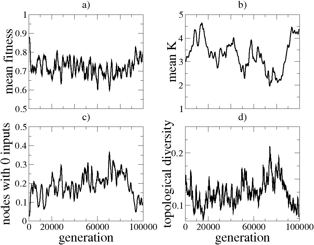
From these data, one can draw the following conclusions:

• The mean fitness and the mean number of inputs per node show large fluctuations over time. This is due to the fact that the last common ancestor of the population is not much more than 50 generations back, which means that the networks in the population are strongly correlated.

• The initial fitness of the population is higher than that at later times. This must be due to the changes occurring in network structure, i.e. to the distribution of the number of inputs becoming broader. In particular, nodes with zero inputs decrease the fitness (see next point).

• There is an anticorrelation between the fitness and the proportion of nodes with 0 inputs. Clearly, a node with 0 inputs does not return to its initial state after a perturbation. If all other nodes did return to the same attractor after a perturbation, the fitness would be identical to the proportion of nodes with at least 1 input.

• There is an anticorrelation between the mean number of inputs and the topological diversity. This is due to the fact that the probability that a given link is mutated becomes smaller when there are more links.

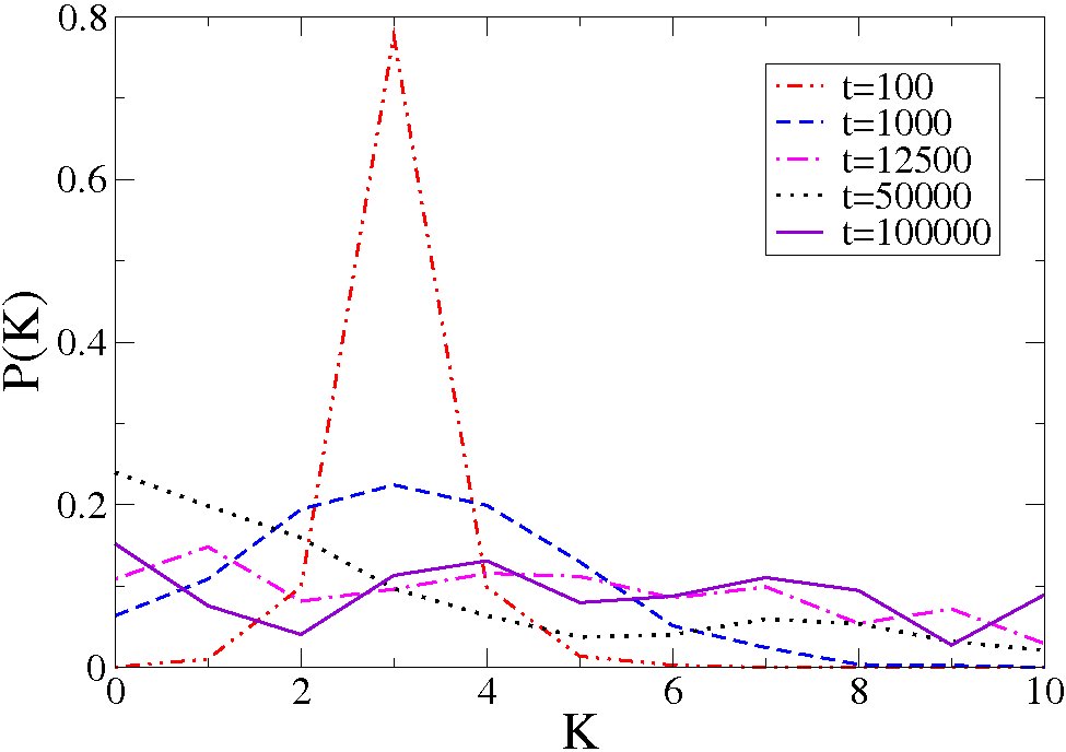
The change in the distribution of the number of inputs is illustrated in Fig. 2. It is becoming broader, with more nodes with zero inputs, which can temporarily even become the dominant type of nodes in the network. (An example for this is given below in one of the cases illustrated by Fig. 3.)

Figure 2: Snapshots of the input distribution at different times during the evolution without selection pressure. The input distribution is changing from a delta peak to a broad distribution with an increased number of nodes with zero inputs.

Let us now apply analytical considerations in order to estimate the topological diversity of the population. Let $T$ be the average time (in terms of the number of generations) to the last common ancestor of two randomly chosen networks in the population. With no selection pressure, we have $T=P$, but with selection this time becomes shorter. Since their last common ancestor, each network received in each generation a mutation with a probability $\mu$. Therefore the two networks together have received on average $2T\mu$ mutations. If the effect of each of them is different and if there are no back mutations, two randomly chosen networks in the population differ on average by $2T\mu$ links and functions. When evaluating the topological diversity, we consider only links. Since three out of four mutations affect links, we expect that two randomly chosen networks in the population have received together $3T\mu/2$ mutations of links. All these mutations affect different links only if $3T\mu/2$ is small compared to the total number of links of a network, $NK$. In this case, the topological diversity should be close to $\dfrac{3T\mu}{2NK}$. Otherwise, it is smaller, since two mutations may affect the same link.

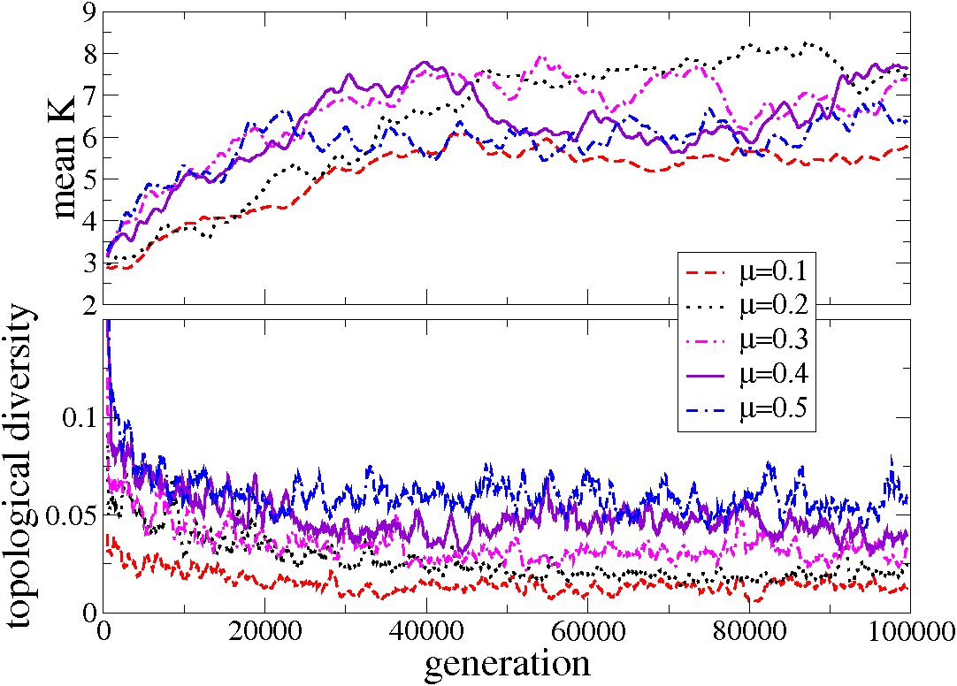
Since $K$ fluctuates strongly with time, the topological diversity fluctuates also and should behave approximately as $1/K$. In figure 1d) we have already seen this anticorrelation. For small $K$, the number of links that are different in the two networks is much smaller than the number of the link mutations they received, and the topological diversity does not become as large as suggested by our simple estimate. This effect is nicely demonstrated by Figure 3, which shows the mean value of $K$ and the topological diversity as function of time for five simulation runs with different mutation rates $\mu$.

Figure 3: Evolution of the mean value of the number of inputs per node (upper figure) and of the topological diversity in the population (lower figure) under no selection pressure and with different mutation rates.

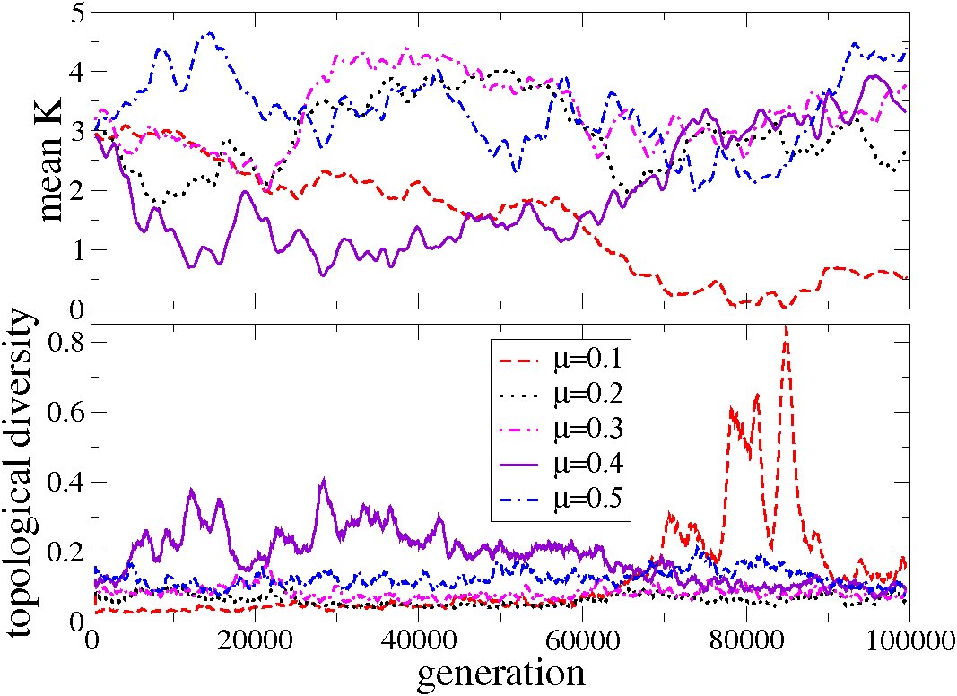
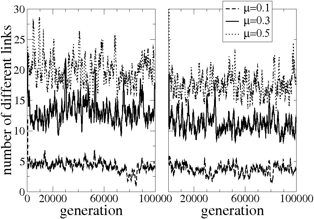
Figure 4 left shows the number of links by which two networks differ on average, which is the topological diversity multiplied by $NK$. Our above simple estimate gives link numbers of 7.5, 22.5 and 37.5 for the mutation rates shown in the figure. These numbers are upper bounds, and one can see that for larger mutation rates and for smaller $K$ values the data are farther below these bounds, since multiple mutations of the same link become more frequent.

Figure 4: Average number of links by which two networks differ, as function of time and for different mutation rates. The selection pressure is zero in the left graph and 100 in the right graph.

We investigated also the influence of the size and of the number of networks in the population on the properties of evolved populations by setting $N$ and/or $P$ to 30. Most of these properties depend strongly on the mean number of inputs per node, which performs a random walk and shows therefore large fluctuations. For this reason, we could not see a clear trend with $N$ or $P$ in the simulation data, although one can expect that the fitness should not depend on $N$ or $P$ and that the fluctuations should decrease with increasing $P$. The diversity should change with $N$ and $P$ as $P/N$, as predicted by analytical estimation earlier in this section.

4 Evolution with very strong selection

Next, we consider the opposite case of very strong selection. In this case, only the networks with the highest fitness value in the population become parents. Now the properties of the fitness landscape play an essential role at determining the evolution of the population. If there were isolated peaks in the fitness landscape, the entire population would perform a hillclimbing process. The fittest individual of the parent population would be the mother of all individuals in the next generation, which would differ from it by at most one mutation. If one of these mutations did lead to a higher fitness, all individuals of the following generation were descendants of the carrier of that mutation. The process would end at a local peak of the fitness landscape, from where no mutation is possible that increases or retains the fitness value.

However, when the fitness landscape has a plateau with maximum fitness that spans the entire network configuration space, the population can contain several individuals with fitness 1, and mutations can generate other genotypes with fitness 1. In our simulations, already the initial population may contain an individual with fitness 1, so that the mean fitness can be close to 1 already after one generation.

Figure 5 shows results of computer simulations for 100000 generations of a population with $N=P=50$ and with a mutation rate $\mu=0.5$. The parameters are the same as in Figure 1, and each data point represents again an average over 1000 generations. We evaluated the same quantities as in the first simulation, except for the number of nodes with 0 inputs, since these do not occur any more. Instead, we show the number of networks with fitness 1 in the population. The proportion of networks with a fitness smaller than 1 must be identical to $\mu$ times the probability that a mutation decreases the fitness of a network with fitness 1.

Figure 5: Evolution of the a) mean fitness, b) mean number of inputs per node, c) mean number of networks with fitness 1, d) proportion of different links in two randomly chosen networks, in the population of 50 networks of 50 nodes each, evolved with the mutation rate 0.5 and high selection pressure.

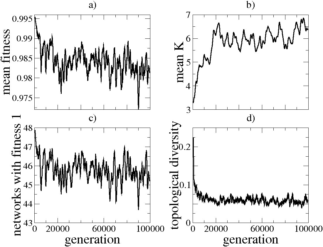
From these data, one can draw the following conclusions:

• The fitness of the population decreases slowly with time. Since all networks with a fitness smaller than 1 must be daughters of networks with fitness 1, this means that at later times the average fitness decrease due to a mutation must be larger.

• The mean number of networks with fitness 1 in the population decreases slowly with time. This means that the probability that a mutation decreases the fitness of the network with fitness 1 is larger at later times.

• The mean number of inputs per node increases slowly but steadily. This was already found in the adaptive walk simulations in Szejka and Drossel (2007). This means that mutations that preserve the maximum fitness are more likely to occur when a link is added than when a link is removed.

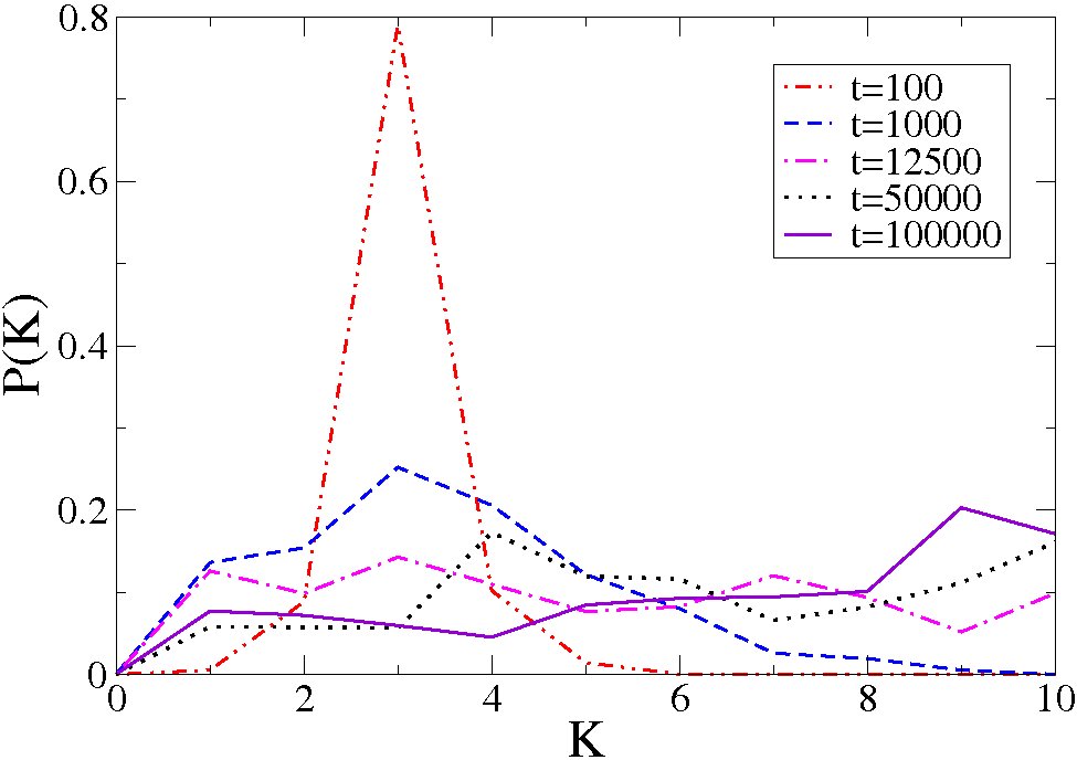
The change in the distribution of the number of inputs is illustrated in Fig. 6. As in the situation without selection, it is becoming broader, but now there are more nodes with higher $K$ and less with smaller $K$. One reason for this is that nodes with zero inputs decrease the fitness, and therefore evolution drives the population into regions in configuration space where such nodes are unlikely to occur.

Figure 6: Snapshots of the input distribution at different times during the evolution. The input distribution is changing from a delta peak to a broad distribution.

Let us now estimate the topological diversity using the arguments from the beginning of Section 3. The number of networks with fitness 1 in the population is defining the effective population size $P^{\prime}$, since only these networks can become parents. From Fig. 5c), we see that this number is around 46 for the parameter values used in this simulation. Correspondingly, the data for the number of links that differ between two randomly chosen networks (Fig. 4 right) are slightly lower compared to the data obtained with zero selection pressure. The estimated upper bound for the topological diversity is now $(3P^{\prime}\mu)/(2NK)$, with deviations from this bound being again larger for smaller $K$ and larger $\mu$. In Figure 7, it can clearly be seen that the topological diversity depends on the mean $K$ value.

Figure 7: Evolution of the mean value of the number of inputs per node (upper figure) and of the topological diversity in the population (lower figure) under strong selection and with different mutation rates.

We explored in more detail the effect of mutations on networks with fitness 1. The probability that a mutation does not decrease fitness is identical to the proportion of networks with fitness 1, shown in Figure 5c). This is because selection pressure is so high that only networks with fitness 1 become parents of the networks in the next generation, each of which then receives a mutation with probability $\mu$. We call a mutation that does not decrease the fitness ”neutral”.

Figure 8: Evolution of the proportion of neutral mutations of different types (upper figure) and of the mean fitness decrease per non-neutral mutation (lower figure) under strong selection pressure and with a mutation rate $\mu=0.5$.

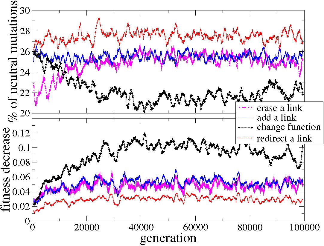
Figure 8 (upper panel) shows the proportion of the four different types of mutations among these neutral mutations, again for $\mu=0.5$. All four types of mutations were chosen equally often, however, the proportion of neutral mutations is different for the four mutation types. The most frequent neutral mutation is the redirection of a link. This means that networks with fitness 1 are most robust (in the sense that their fitness is not decreased) to this type of mutations. The least frequent neutral mutation is initially the deletion of a link; at later times the change of a function is least frequent. The combined contribution of these two types of mutations to the neutral mutations is approximately constant in time. The frequency of mutations that add a link is also approximately constant. This implies that the slow increase of the mean $K$ value is not due to a beneficial effect of mutations that add links, but due to the fact that erasing a link decreases the fitness more often than the addition of a link, in particular in the beginning of the simulation, where also the largest increase of $K$ can be seen. At later times, deletions and additions are equally frequent among the neutral mutations. The increase of $K$ explains why mutations that change the canalyzing function become less frequent among neutral mutations. When $K$ is larger, such a change affects more nodes on an average.

In Figure 8 (lower panel), we show the amount by which fitness decreases due to a non-neutral mutation. This amount increases with time for all four types of mutations. This must be due to the fact that the perturbation of one node affects more nodes when $K$ is larger, and therefore a mutation affects also more nodes. For the same reason, mutations that change the canalyzing function lead to a larger fitness decrease than other mutations. The redirection of a link leads to the smallest fitness decrease because it does not involve changes in the update functions.

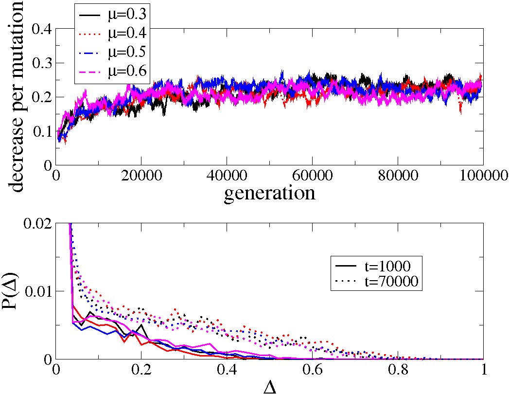
Next, we investigated the influence of the mutation rate on these results. Figure 9 (top) shows the fitness decrease per mutation for different mutation rates. Here, we now do not discriminate between different types of mutations. The mean fitness decrease per non-neutral mutation appears to be independent of the mutation rate with which the networks were evolved.

The lower graph of Figure 9 shows the probability distribution of the fitness decrease per mutation at an early and at a late time. Here, neutral mutations, which lead to a fitness decrease of 0, are also included. After approximately 30000 generations, the probability distribution of the fitness decrease reaches a stationary shape. This shape does not depend on the mutation rate with which the networks were evolved. Most of the mutations do not decrease fitness or they decrease it by the smallest possible amount of 0.02 (which means that only after 1 out of the $N$ possible perturbations the network does not return to the same attractor). We do not show completely this part of the curves in order to make the distribution for larger fitness decreases better visible. There are no significant differences between the curves for different $\mu$. We have already discussed above that the mean fitness decrease per non-neutral mutation is larger at later times, when $K$ is larger.

Figure 9: Upper graph: Fitness decrease per (non-neutral) mutation as function of time, for four different mutation rates. Lower graph: Probability distribution of the fitness decrease $\Delta$ (including zero decrease) due to a mutation, evaluated at two different times during evolution.

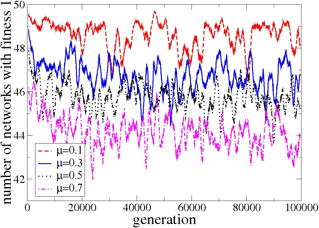
While networks evolved with different mutation rates do not differ in the fitness decrease per (non-neutral) mutation, they do differ in other respects. Figure 10 shows the number of networks with fitness 1 in the population as function of time for four different mutation rates. If the probability of a mutation being neutral was the same in all four cases, the distance of the curves from the value 50 should be proportional to $\mu$. Due to the large fluctuations, the data cannot give a clear answer to whether this is the case. We therefore evaluated directly the probability that a mutation decreases fitness, for mutation rates ranging from $\mu=0.1$ to $\mu=0.7$. These data show a clear trend, with networks evolved with higher mutation rates being less likely to decrease their fitness under a mutation. They are more robust to mutations. Fig. 11, upper panel, shows the curves obtained with $\mu=0.3$ and 0.6. This means that the networks on the plateau of the fitness landscape, reached by evolution under strong selection, have different properties depending on the mutation rate with which they were evolved. This result is not merely due to the fact that populations evolve slower when the mutation rate is smaller. If this were the case, the curves obtained with a smaller mutation rate should resemble those obtained with larger mutation rates at an earlier time.

Figure 10: Change of the number of networks with fitness 1 in the population during evolution with different mutation rates and high selection pressure

Figure 11: Evolution of the percentage of mutations decreasing fitness (upper graph) and of the mean attractor length in the population (lower graph) under strong selection and with two different mutation rates.

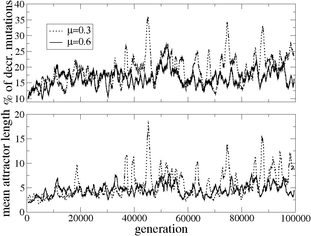
There is a correlation between the mean attractor length and the frequency of neutral mutations, as revealed by the lower graph of Fig. 11. This correlation can be seen most clearly by comparing the positions of the peaks. The numerical values of the correlation between the two curves are 0.892 for $\mu=0.3$ and 0.885 for $\mu=0.6$. These values are not far from the value 1, which would result if the two curves were proportional to each other. This means that networks with longer attractors are more likely to decrease their fitness under mutations, which is not too surprising. Conversely, networks that are more robust against mutations have smaller attractors.

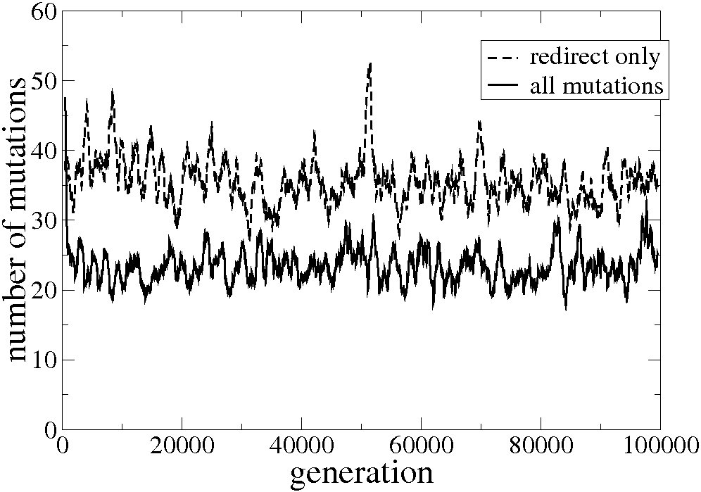
In order to investigate how evolution proceeds when there can be no slow change in network structure, we also performed simulations with a different rule, which allows no deletion and addition of links or changes of functions, but only the redirection of the links. In this situation, the number of inputs of every node remains 3, and the distribution of the number of outputs remains Poissonian. The population reaches quickly the stationary fitness value, and the diversity of the population is still large.

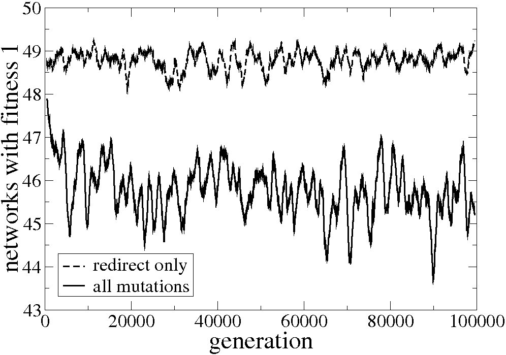
In Figure 12 the mean number of networks with fitness 1 in a population obtained with this new mutation rule is compared to the results obtained with the original rules, for $P=50$ and $\mu=0.5$. The data imply that the mean fitness decrease per mutation is much larger for the original rule. We have seen (Fig. 8) that when the networks are evolved with all four types of mutations, those mutations redirecting links are decreasing the fitness less than others. Redirections of links could also have smaller effect on the fitness of the networks evolved under the new rule, which would then explain the observed difference.

Figure 13 shows the number of mutations by which two randomly chosen networks of a population differ, as function of time, for the two mutation rules. This number is considerably larger when links are only rewired. We attribute this result to the larger effective population size and to the absence of networks with small average $K$ values.

Not surprisingly, we do not find any long-term trend in the mean fitness of the population with the modified mutation rule. This confirms our suggestion that the long-term change of the network structure is responsible for the slow and steady decrease of the fitness in the original simulations.

Figure 12: Number of networks with fitness 1 as function of time for high selection pressure ($p=100$) and the mutation rate $\mu=0.5$. The original model is compared with a model where only the redirection of links is allowed.

Figure 13: Number of mutations by which two randomly chosen networks of a population differ, as function of time, for the two mutation rules. The parameters are again $p=100$ and $\mu=0.5$.

Finally, we investigated the influence of the size and of the number of networks in the population on the properties of evolved populations by setting $N$ and/or $P$ to 30. We found that the mean fitness of the population decreases with decreasing $N$, since a node is more likely to be affected by a mutation when $N$ is smaller. A decrease of the population size shows even larger effect on the mean fitness, because the influence of genetic drift becomes more important compared to the influence of selection. Earlier in this Section we estimated that the topological diversity should change approximately as $P/N$. In our simulations, we find trends that agree with this assumption. However, due to large fluctuations, we cannot make the statements of this paragraph more quantitative.

5 Evolution with finite selection pressure

When selection pressure is finite, the properties of the evolving populations should be between the two extreme cases studied until now. When mutation rates are too high, selection pressures too low, or population sizes too small, the effect of selection is hardly visible in the population, the evolution of which is then dominated by drift.

Figure 14: Evolution of the mean fitness for different selection pressures and a mutation rate $\mu=0.2$.

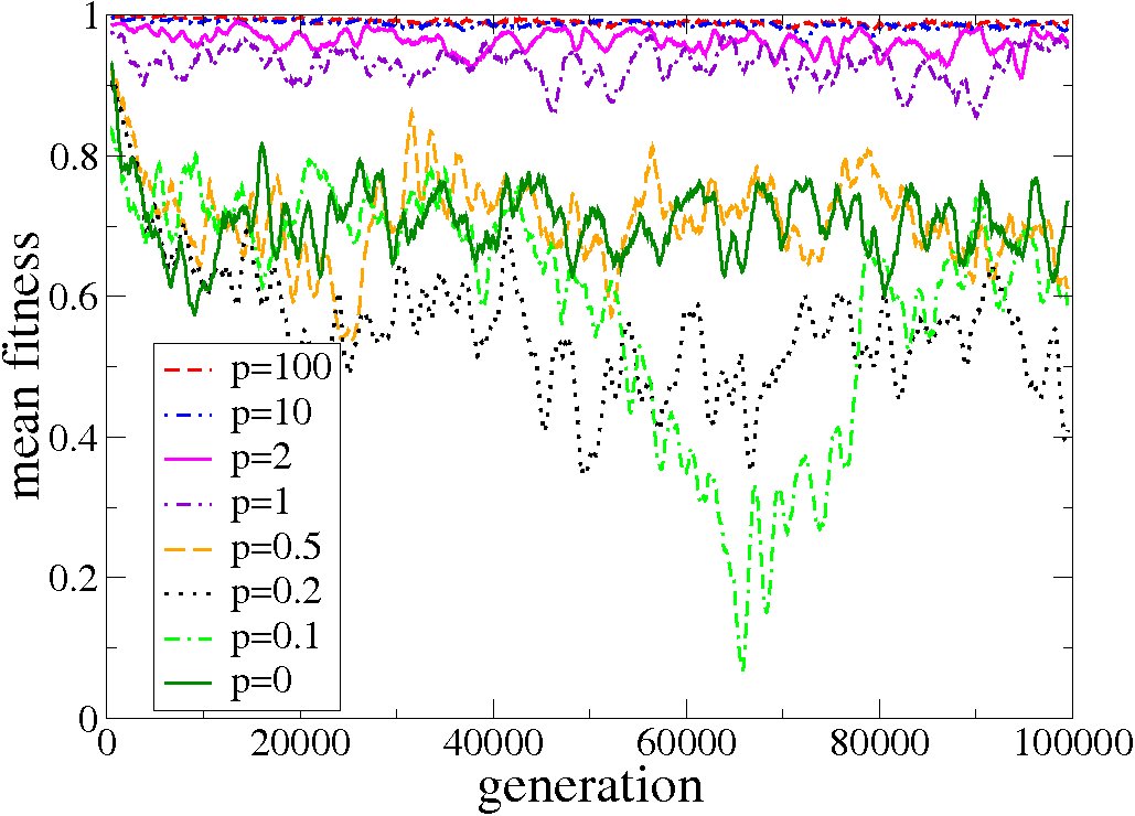
Figure 14 shows the mean fitness of a population with $N=P=50$ and a mutation rate $\mu=0.2$ as a function of time for different values of the selection pressure $p$. One can clearly see that for $p\leq 0.5$ the evolution of the fitness resembles that of the system with $p=0$, which means that drift dominates the evolutionary process. The simulation for $p=0.1$ accidentally goes through a stage where there are very many nodes with 0 inputs ( this is correlated with the decrease of the mean $K$ value that can be seen in Fig.15), resulting in a very low fitness.

Figure 15: Evolution of the mean number of inputs per node under different selection pressures and mutation rate 0.2

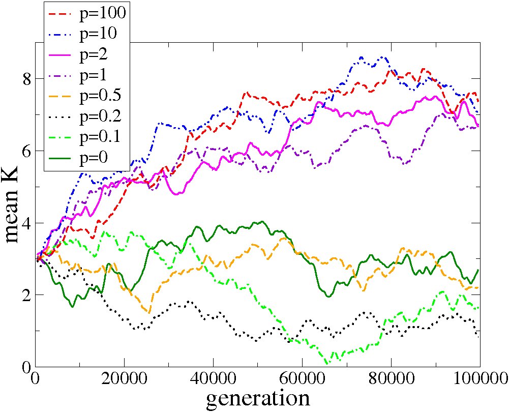
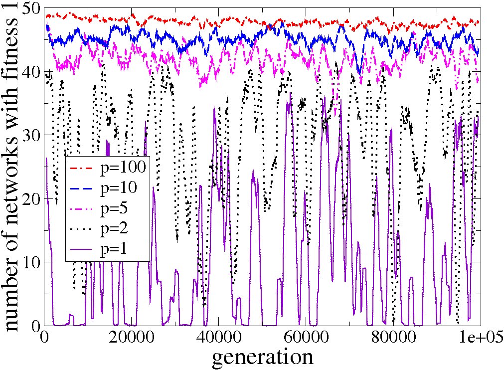
For $p\geq 1$, selection has a clear effect on the fitness. Figure 16 shows the number of networks with fitness 1 in the population as a function of time for $p\geq 1$. (For $p\leq 0.5$, there are almost no networks with fitness 1.) When the selection pressure is smaller, this number is also smaller. Just as for the case of very large selection pressure, the populations show a slow and slight decrease of the mean fitness with time. This decrease is again correlated with an increase in the mean connectivity, as shown in Figure 15.

Figure 16: Change of the number of networks with fitness 1 during the evolution under different selection pressures and mutation rate 0.2

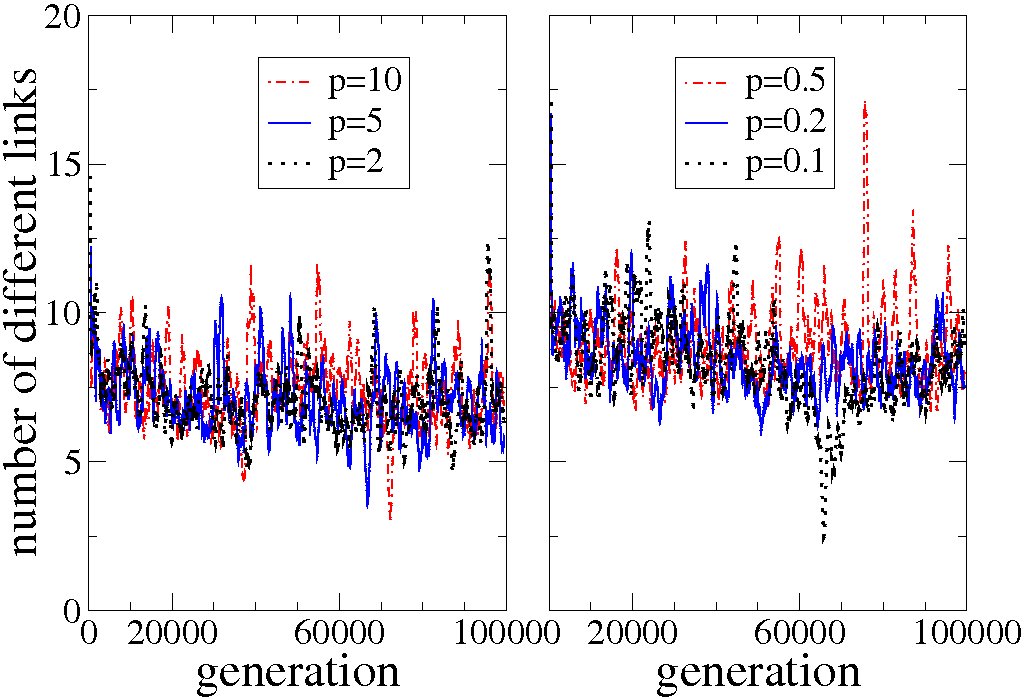
The topological diversity is again strongly correlated with the number of inputs per node. In Figure 17 we show the number of links by which two randomly chosen networks of the population differ. This number does not depend on $K$, but on the effective population size. It has approximately the same mean value for all selection pressures, whether they are weak or strong. This is not surprising, as we have already seen that the effective population sizes do not change much when the selection pressure is changed from 0 to a very high value. For weak selection, there are instances where the total number of links becomes very small.

Figure 17: Number of links by which two randomly chosen networks differ in the population during evolution with mutation rate 0.2 and under selection pressures $p\geq 1$ (left) and $p\leq 0.5$ (right).

6 Conclusions

We have investigated the evolution of populations of random Boolean networks under selection for robustness of the dynamics with respect to the perturbation of a node. The fitness landscape of such a model contains a huge plateau of maximum fitness that spans the entire network space.

Even in the absence of selection, we found long-term changes in the network structure. In particular, the distribution of the number of inputs became broad, leading to a decrease in the mean fitness. Furthermore, since links are randomly added or deleted during mutations, the evolutionary process may go through periods where there are very few links in the networks, which implies that fitness is particularly low.

When selection is so strong that only networks with the maximum fitness value 1 can become parents of the next generation, the evolutionary process is accompanied by a slow increase in the mean connectivity and a slow decrease in the mean fitness, lasting for several 10000 generations. In fact, this process was apparently not fully finished at the end of our long-term simulations. We ascribe this long-term trend to the fact that nodes with 0 inputs do not return to their initial state after a perturbation. They decrease the fitness of the network, and therefore mutations that add links are favoured with respect to mutations that remove links. Interestingly, the mean fitness of the population decreases nevertheless. This resembles the ’tragedy of commons’ Hardin (1968), where the mean fitness of the population decreases, while each individual strives to obtain maximum fitness. But in contrast to the ’tragedy of the commons’, the fitness of an individual in our model does not depend on the other individuals. This effect can in our model be explained by the fact that networks with more links per node are more likely to decrease their fitness when a mutation is performed.

We found furthermore that populations evolved with higher mutation rates show a higher robustness against mutations, i.e., they are less likely to loose fitness under a mutation. This means that even though all the evolved populations move on the plateau of maximum fitness, they end up in different regions of network space. Robustness against mutations evolves because networks with higher mutational robustness have more offspring in the next generation. This trend is countered by the generation of mutationally less robust networks through neutral mutations. When the effect of mutations becomes more important (because mutation rates are higher), the equilibrium point between these two trends moves towards higher mutational robustness. This explains why networks evolved under higher mutation rates are more robust against mutations. We found that higher robustness against mutations is accompanied by a shorter mean attractor length. Obviously, higher mutational robustness is also correlated with higher dynamical robustness, i.e. with higher mean fitness. The above-mentioned slow decrease (after the initial increase towards the plateau) in the mean fitness of the population is therefore reflected in a similar slight decrease in mutational robustness.

Populations evolved at finite selection pressures behave similarly to those without selection when drift dominates over selection, and they behave similarly to those with high selection pressure when the effect of selection dominates over drift.

Let us now compare the features of our model with those of real gene regulation networks. The perturbation of the state of a node can be interpreted as an effect of the omnipresent thermal noise and stochastic fluctuations of molecular concentrations. Real gene regulation networks have to maintain their function under such perturbations. This dynamical robustness should be preserved during evolutionary processes, even when the phenotype of the mutant individual is different from that of the parent. Indeed, experimental studies show robustness of cellular networks under mutations. The gene regulation network of Escherichia coli Isalan et al. (2008), and the phage $\lambda$ regulatory circuitry, Little et al. (1999), preserved their function under different changes in their structure, implying high robustness under mutations and high dynamical robustness after the mutations. These findings suggest that the fitness landscape of real cellular networks also contains a huge plateau of high fitness, through which the networks can move without loss of functionality.

Other studies of the evolution of Boolean networks show also a connection between dynamical robustness and mutational robustness. In Wagner (1996); Ciliberti et al. (2007); Kaneko (2007); Sevim and Rikvold (2008), the authors find that robustness to noise (i.e., to small perturbations of the state of the network) and robustness to mutations are highly correlated. In those investigations, mutational robustness and dynamical robustness evolve together and increase with time.

The results of our study make it plausible that there is a plateau at the global maximum of fitness landscape of real genetic regulatory networks. We have seen that in such a landscape networks can evolve without loss of dynamical robustness, i.e., of functionality. Their evolution is therefore driven by the demand for achieving high mutational robustness. The evolved networks are therefore robust to changes in their structure, being in the same time able to preserve their function under small environmental changes. When evolution occurs with higher mutation rates, networks can continue to function only when their mutational robustness is sufficiently large. Our simulations indicate that an increased mutational robustness evolves naturally when mutation rates are higher. In order to remain evolvable, networks also have to preserve variability. This is the case in our simulations, since mutations can change the phenotype (i.e., the attractors) even after a long time.

We thank Agnes Szejka for useful discussions.

References

- Drossel (2001) B. Drossel, Adv.Phys. 50, 209 (2001).
- Fontana et al. (1993) W. Fontana et al., Phys. Rev. E 3, 2083 (1993).
- Schuster et al. (1994) P. Schuster, W. Fontana, P. Stadler, and I. Hofacker, Proc. Roy. Soc. Lond. B 255, 279 (1994).
- Bastolla et al. (2003) U. Bastolla, M. Porto, H. Roman, and M. Vendruscolo, J. Mol. Evol. 57, 103 (2003).
- Kauffman (1969a) S. Kauffman, J. Theor. Biol. 22, 437 (1969a).
- Kauffman (1969b) S. Kauffman, Nature 224, 177 (1969b).
- Frank (1999) S. Frank, J. Theor. Biol. 197, 281 (1999).
- Wagner (1996) A. Wagner, Evolution 50, 1008 (1996).
- Sevim and Rikvold (2008) V. Sevim and P. Rikvold, J. Theor. Biol. 253, 323 (2008).
- Aldana et al. (2007) M. Aldana, E. Balleza, S. Kauffman, and O. Resendiz, J. Theor. Biol. 245, 433 (2007).
- Kauffman and Smith (1986) S. A. Kauffman and R. G. Smith, Physica D 22, 68 (1986).
- Stern (1999) M. D. Stern, Proc. Natl. Acad. Sci. USA 96, 10746 (1999).
- Oikonomou and Cluzel (2006) P. Oikonomou and P. Cluzel, Nature Physics 2, 532 (2006).
- Lemke et al. (2001) N. Lemke, J. C. M. Mombach, and B. E. J. Bodmann, Physica A 301, 589 (2001).
- Bornholdt and Sneppen (1998) S. Bornholdt and K. Sneppen, Phys. Rev. Lett. 81, 236 (1998), eprint physics/9708026.
- Bornholdt and Sneppen (2000) S. Bornholdt and K. Sneppen, Proc. R. Soc. Lond. B 267, 2281 (2000), eprint cond-mat/0003333.
- Paczuski et al. (2000) M. Paczuski, K. E. Bassler, and A. Corral, Phys. Rev. Lett 84, 3185 (2000), eprint cond-mat/9905082.
- Luque et al. (2001) B. Luque, F. J. Ballesteros, and E. M. Muro, Phys. Rev. E 63, 051913 (2001), eprint cond-mat/0102396.
- Bornholdt and Rohlf (2000) S. Bornholdt and T. Rohlf, Phys. Rev. Lett. 84, 6114 (2000), eprint cond-mat/0003215.
- Liu and Bassler (2006) M. Liu and K. E. Bassler, Phys. Rev. E 74, 041910 (2006), eprint cond-mat/0605020.
- Szejka and Drossel (2007) A. Szejka and B. Drossel, Eur. Phys. J. B 56, 373 (2007), eprint q-bio/0701025v1.
- Moreira and Amaral (2005) A. A. Moreira and L. A. N. Amaral, Phys. Rev. Lett. 94, 218702 (2005), eprint cond-mat/0504722.
- Hardin (1968) G. Hardin, Science 162, 1243 (1968).
- Isalan et al. (2008) M. Isalan, C. Lamerle, K. Michalodimitrakis, C. Horn, P. Beltrao, E. Raineri, M. Garriga-Canut, and L. Serrano, Nature 452, 840 (2008).
- Little et al. (1999) J. Little, P. Shepley, and D. Wert, EMBO J. 18, 4299 (1999).
- Ciliberti et al. (2007) S. Ciliberti, O. Martin, and A. Wagner, PLoS Comput. Biol. 3, 164 (2007).
- Kaneko (2007) K. Kaneko, PLoS ONE 2, e434 (2007).