Scaling of degree correlations and the influence on diffusion in scale-free networks
Abstract
Connectivity correlations play an important role in the structure of scale-free networks. While several empirical studies exist, there is no general theoretical analysis that can explain the largely varying behavior of real networks. Here, we use scaling theory to quantify the degree of correlations in the particular case of networks with a power-law degree distribution. These networks are classified in terms of their correlation properties, revealing additional information on their structure. For instance, the studied social networks and the Internet at the router level are clustered around the line of random networks, implying a strongly connected core of hubs. On the contrary, some biological networks and the WWW exhibit strong anti-correlations. The present approach can be used to study robustness or diffusion, where we find that anti-correlations tend to accelerate the diffusion process.
pacs:
89.75.Fb, 89.75.Da, 87.23.GeThe topological structure of complex networks is largely determined by the way in which the constituent units are interconnected. Correlations in the connectivity of complex networks have been proved to be important and have been used to explain the functionality, robustness, stability, and structure of networks from Biology maslov and Sociology newman2 to Computer Science vespignani2 . A study of the correlation profile in a network of protein-protein interactions revealed that links from hubs to non-hub nodes are favored maslov , a result with consequences for the stability and the modularity in biological networks. In the case of social networks, Newman has shown that most of them are assortative (i.e. hub-hub correlations dominate the system) newman2 , and Colizza et al. demonstrated the ‘rich-club’ phenomenon where all hubs tend to form a connected cluster Colizza . As a result, social networks are more difficult to immunize and diseases can spread fast.
Recently, it was also shown that hub anticorrelations, i.e. the tendency of the hubs not to be directly connected with each other, give rise to fractal networks shm , such as the undirected (symmetrized) WWW, the protein homology network homology and other biological networks. On the contrary, when there is a large probability of direct hub connections the resulting networks, such as the Internet, the cond-mat co-authorship and other social networks, are non-fractals shm2 . In this category falls also the random configuration model Molloy ; ba .
An important topological feature of complex networks is the degree distribution , where is the number of links for a given node. Although the form of has a direct influence on the network properties, it cannot convey all the information for the network structure. Thus, two networks can have the same distribution but with completely different topologies, determined by the presence of degree correlations. This structure can be captured by the probability that two nodes of degree and are connected to each other, and by quantities derived from , such as the Pearson coefficient , the average degree of nearest neighbors , etc.
Despite their importance, a general theoretical framework to describe and characterize degree correlations in scale-free networks is still work in progress. For an attempt to describe correlations using a master equation approach see redner . Here, we find that the degree correlations in the studied scale-free networks can be characterized in terms of a correlation exponent , which we calculate using a renormalization approach. This allows us to propose a classification of a set of dissimilar networks, according to the degree of correlations into a small number of different classes in a “phase diagram”. For example, biological networks and the WWW are in the strong anti-correlations part of the diagram, while social networks and the Internet are clustered near the region of random networks. We show how we can use these ideas to explore more network properties, such as diffusion and robustness, which depend on the degree of correlations in the network.
We start by recalling the renormalization of a network under a scale transformation. The renormalization procedure tiles a network according to the box-covering algorithm sghm , with the minimum number of boxes where the maximum distance in any box is less than . Each box is subsequently replaced by a node, and links are established between these new ‘super-nodes’ if at least one node included in a box was connected to any node of the other box. These boxes are treated as the nodes of the renormalized network. Renormalization is a reliable method for determining how the network behaves at different length scales. Self-similarity is then obtained if the network structure remains invariant under the renormalization.
Alternatively, we can retain multiple links between the boxes when we renormalize a network maslov2 . As we show below, though, this is not a strong effect, mainly due to preservation of the self-similar structure under renormalization. In contrast, during a random rewiring process degree correlations are destroyed, but bias is introduced if multiple links are forbidden.


We use renormalization and scaling theory to determine the form of . Since the self-similarity of a scale-free network requires the invariance of the degree distribution , a power-law distribution of , where is the degree exponent, is the only form that can satisfy this condition shm . Taking this idea one step further, it is interesting to clarify whether correlations between degrees, as expressed by the joint degree distribution , also remain invariant. In Fig. 1 we present an example of this distribution before and after renormalization for the WWW and the Internet at the router level (similar results are derived for other networks, as well). Allowing multiple links between boxes does not significantly modify the result. The statistical similarity of the corresponding plots suggests the invariance of . Accordingly, this suggests that the and dependence can be separated and the behavior of the tail of the joint degree distribution is:
| (1) |
The value of the first exponent in Eq. (1) is obtained from the density conservation law: Equation (1) is also consistent with the known result for completely random networks
| (2) |
i.e. the exponent for these networks is , as expected from the symmetry in this case. Eq. (1) is also consistent with previous findings in Ref. maslov . The probability distribution for the neighbor connectivity in the yeast protein interaction network was there shown to behave differently for low-degree nodes, where the -dependence was , and for large-degree nodes, with a dependence. Using Eq. (1) we can see that integrating over for low-degree nodes () we retrieve the dependence. For the case of hubs, where integration is over , the dependence on the degree is and for the yeast protein interaction network we have calculated that (see Fig. 3). These results are in agreement with the observed behavior in maslov .
Next, we introduce a scale-invariant quantity to simplify the estimation of , even for small networks. We are motivated to introduce this quantity by asking whether a node is significantly linked to more connected nodes, i.e. a node considers another node as a ‘hub’ if its degree is much larger than its own. We define the ratio
| (3) |
as the measure of a node’s preference to connect to neighbors with degree larger than ( is an arbitrary positive number, and large corresponds to the identification of the hubs) footnote . From the scaling of with , we are able to obtain the exponent in a simpler way than using , which presents more fluctuations than the average quantity . The conditional probability is . We find for a scale-free distribution:
| (4) |
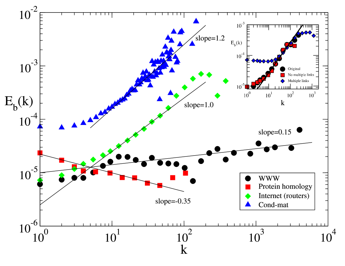
We have verified that the scaling of remains invariant under renormalization. The same scaling exponents are recovered for the renormalized networks, even when multiple links are allowed between two boxes (Fig. 2 inset). In the latter case, the renormalized nodes have in general larger degrees, which means that deviations appear in nodes of smaller degree. Additionally, was found to be independent of the value of . We notice that other quantities derived from may not be invariant under renormalization, such as or , and therefore are not suitable to distinguish fractal from non-fractal networks.
In Fig. 2 we present the behavior of for the WWW, protein homology, Internet (router level) and cond-mat authorship. The existence of a scaling relation over a range, combined with the invariance of this curve, support Eq. (4) and the form used for in Eq. (1). The WWW and the protein homology network have been shown to have a fractal topology. The slope of with is small or negative in these cases with values of and , respectively. This behavior is in contrast with the two non-fractal networks in the figure, i.e. the Internet at the router level and the cond-mat co-authorship network, where increases almost linearly with increasing . For these networks we find that and , respectively.

In order to interpret the values of we now turn to the renormalization scheme shm . After renormalization the number of nodes in the network and the degree of a node scale with as power laws with fractal exponent and degree exponent , respectively (we use a prime to describe quantities measured in the renormalized network):
| (5) |
If and are finite, the network is fractal. If and (or equivalently the decay is exponential or faster) the network is not fractal.
After tiling the network with boxes of diameter , each of these boxes have one unique local hub (i.e. the largest degree node in the box). Considering all possible pairs of boxes, we introduce the probability that there exists a direct connection between the two hubs of any two boxes. We have shown (see e.g. Figs. 2e, 3d of Ref. shm2 ) that the probability scales with the length as
| (6) |
Below we relate the exponent to the hub-hub repulsion through the hub correlation exponent , which is crucial for fractality.
The conservation of links in the renormalized network leads to the expression
| (7) |
Using Eqs. (1), (5), (6), and (7) we get the relation which finally leads to
| (8) |
where we have substituted the value . This relation of with shows that correlations between the hubs of the boxes determine the correlations for all degrees, in accordance with the invariance under renormalization.
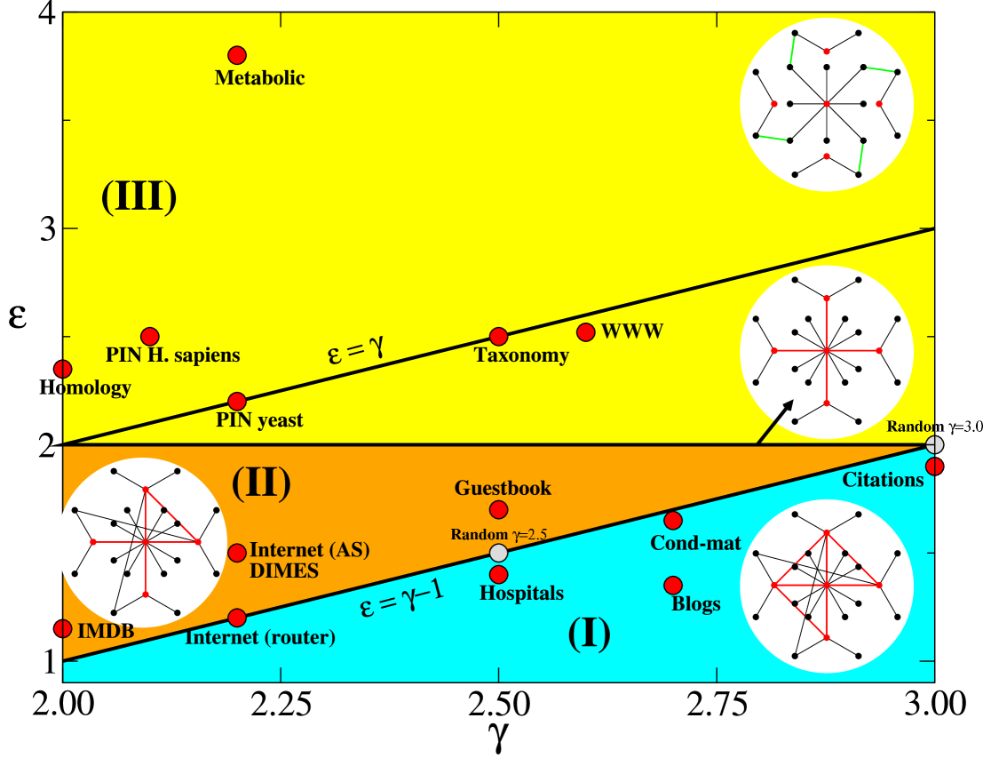
The direct determination of through the slope of vs enables us to construct a ‘phase diagram’ in the plane , shown in Fig. 3. This plot is classifying the studied networks in classes according to their degree of correlations, even though they correspond to dissimilar systems in biology, sociology or technology.

As shown in Eq. (2), the exponent for a random network corresponds to the random line , which is verified in the plot for different values of the configuration model. In random network models, correlations arise because links are selected for connecting with each other equiprobably, so that the probability of two hubs being connected is large catanzaro . Thus, networks that are close to the line exhibit hub-hub correlations. The random line separates the diagram in two main parts: (a) above the line where the hub correlations tend to become weaker, and (b) below the line where networks have even larger correlations (hubs are connected to each other with even higher probability than the one corresponding to a randomly created structure).
In the diagram, the social networks and the Internet at the router level are clustered around the line . This is an indication that there is a strongly connected core of hubs in these systems, consistent with previous studies. The biological networks and the WWW, on the other side, are far away from the random line. This implies that there is a richer structure in these networks with hubs separated from each other. The distance in the plot from quantifies how different from randomness the network structure is, in terms of degree correlations.
As increases from , we expect that at some point the networks will become fractal, due to increased hub-hub correlations. The point of emergent fractality is found through Eq. (8), where the borderline case of yields . Indeed, we have verified via direct measurements of that all the networks above the line in Fig. 3 are fractals.
Thus, starting from we can separate the phase space into areas where the hub correlations are stronger than in random models (area I) or weaker than that (areas II and III). The weak correlation areas II and III are further divided by the line which determines whether the anticorrelations are strong enough to result in a fractal network (III) or not (II).
An immediate result from this diagram is the different position of the Internet at the router level compared to the AS level vazquez . Although the degree distribution of these two networks is the same (), the correlation exponent reveals that there are more hub-hub connections at the router level, similar to the case of a random network. Contrary to that, the AS level exhibits a structure with less correlations deviating from that of a simple random model. This difference may hint on different design principles or requirements at varying levels of the Internet.

The above approach can be directly applied to explore many interesting properties, such as network robustness, synchronization, or diffusion processes. Until now, theoretical studies have been limited to using the uncorrelated version of . The introduction of Eq. (1) enables us to substitute this form and generalize the problem for networks with known correlation exponents. For example, we can study the effect of correlations on diffusion by starting with the master equation for the density of particles on nodes with degree at time
| (9) |
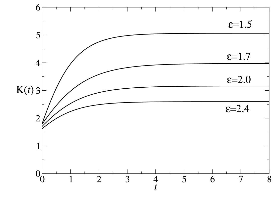
and substitute with a form derived through Eq. (1). The Laplace transform of the above equation leads to a Fredholm integral equation of the second kind with separable kernel that can be solved analytically. We define the quantity , where , and serves as a measure of the diffusing particles preference to larger or smaller degrees . The analytical result for , defined as , is , where and are constants depending on and , while . The result for is displayed in Fig. 4 for networks with . The exponential convergence to the asymptotic steady-state configuration depends on the value of , which increases with the exponent . Networks that are close to the random case require longer times for reaching the equilibrium state and the diffusing particles prefer to occupy larger degree nodes. A larger value enhances anti-correlations in the network and the particles move faster occupying smaller degree nodes on the average. We can infer, thus, that stronger correlations tend to speed up the diffusion process. The mechanism behind this behavior is as follows: when the hubs are directly connected to each other the particles tend to remain localized in the neighborhood around these hubs, so that it takes longer for them to explore wider areas. On the contrary, when hub anti-correlations are important the particles spend most of their time in the intermediate areas which are formed by smaller degree nodes and which connect indirectly the hubs to each other.
Acknowledgements.
We acknowledge valuable discussions with Shlomo Havlin and support from NSF grants.References
- (1) S. Maslov and K. Sneppen, Science 296, 910 (2002).
- (2) M.E.J. Newman, Phys. Rev. Lett. 89, 208701 (2002).
- (3) R. Pastor-Satorras, A. Vázquez, and A. Vespignani, Phys. Rev. Lett. 87, 258701 (2001).
- (4) V. Colizza, A. Flammini, M.A. Serrano, and A. Vespignani, Nature Physics 2, 110 (2006).
- (5) C. Song, S. Havlin, and H.A. Makse, Nature 433, 392 (2005).
- (6) A.T. Adai, S.V. Date, S. Wieland, and E.M. Marcotte, J. Mol. Biol. 340, 179 (2004).
- (7) C. Song, S. Havlin, and H.A. Makse, Nature Physics 2, 275 (2006).
- (8) M. Molloy and B.A. Reed, Random Struct. Algorithms 6 161 (1995).
- (9) A.-L. Barabási and R. Albert, Science 286, 509 (1999).
- (10) P. Krapivsky and S. Redner, Phys. Rev. E 63, 066123 (2001).
- (11) C. Song, L. K. Gallos, S. Havlin, and H. A. Makse, J. Stat. Mech. P03006 (2007).
- (12) S. Maslov, K. Sneppen, and A. Zaliznyak, Physica A 333, 529 (2004).
- (13) Notice that we could have defined without using the denominator in Eq. (3), i.e. , in which case we get . However, due to the large fluctuations occurring at the tails of the degree distribution in real-life networks, the calculation of through Eq. (3) was proved to be more robust.
- (14) M. Catanzaro, M. Boguna, and R. Pastor-Satorras, Phys. Rev. E 71 027103 (2005).
- (15) A. Vazquez, R. Pastor-Satorras, and A. Vespignani, cond-mat/0206084.
- (16) A description of the databases used in Fig. 3 and citations to their source can be found at http://jamlab.org .