Reduced fidelity susceptibility in the one-dimensional transverse field Ising model

Abstract

We study critical behaviors of the reduced fidelity susceptibility for two neighboring sites in the one-dimensional transverse field Ising model. It is found that the divergent behaviors of the susceptibility take the form of square of logarithm, in contrast with the global ground-state fidelity susceptibility which is power divergence. In order to perform a scaling analysis, we take the square root of the susceptibility and determine the scaling exponent analytically and the result is further confirmed by numerical calculations.

I Introduction

Within the last few years, some concepts and tools in the field of quantum information science Nielsen and Chuang (2000), such as entanglement and fidelity, have been introduced in the study of quantum phase transitions (QPTs) Sachdev (1999), which are described traditionally in terms of order parameters and symmetry breaking. However, without a priori knowledge of the order parameter, when a system undergoes QPT, its ground state will change dramatically. Since the definition of fidelity is the overlap between two quantum states, it’s natural to introduce it in the field of QPTs. The most studied fidelity is the global ground state fidelity Quan et al. (2006); Zanardi and Paunković (2006); Buonsante and Vezzani (2007); Zanardi et al. (2007); Cozzini et al. (2007); Venuti and Zanardi (2007); Zanardi and Cozzini (2007); You et al. (2007); Chen et al. (2008); Zhou and Barjaktarevic (2007); Zhou et al. (2007); Gu et al. (2007); Chen et al. (2007); Ning et al. (2008); Kwok et al. (2008a); Yang (2007); Zhao and Zhou (2008); Yang et al. (2008); Zhou (2007), which is an overlap between two ground states with a slight change of the parameters. Therefore, to avoid the arbitrariness of the small change in numerical computation, Zanardi et al. introduced the Riemannian metric tensor Venuti and Zanardi (2007); Zanardi and Cozzini (2007), while You et al. suggested the fidelity susceptibility You et al. (2007), which is an effective tool to study the critical properties.

So far, in most works, people have concerned with the global ground state fidelity. We note that as far as in Ref Znidaric and Prosen (2003) the authors have introduced a reduced fidelity which is defined as the trace of the product of two matrices. This definition is not rigorous in quantum-information theory, and they require one of the density matrices to be a pure state to agree with the rigorous mixed state fidelity Uhlmann (1976). While in this paper, the reduced fidelity we used is defined rigorously in quantum-information theory and is studied in Zhou (2007); Gorin et al. (2006); Paunkovic et al. (2008); Ma et al. (2008); Kwok et al. (2008b). It has been shown that the reduced fidelity susceptibility (RFS) is an efficient indicator of QPTs.

In this paper, we study the scaling and critical behaviors of the RFS of two neighboring sites in the famous one-dimensional (1D) transverse field Ising model (TFIM). We note that the quantum critical properties of some other quantities like concurrence  Osterloh et al. (2002) and von Neumann entropy  Su et al. (2006), and the global ground state fidelity susceptibility Chen et al. (2008) have been studied in this model. However, the scaling and critical behaviors of them are quite different from the RFS for two neighboring sites . It’s found that the scaling and critical behaviors of the RFS take the form of square of logarithm as $(\ln N)^{2}$ for finite-size system and $(\ln|\lambda-1|)^{2}$ ($N$ is the total number of spins and external parameter $\lambda=1$ is the critical point) in the thermodynamic limit, in contrast with the global fidelity susceptibility Chen et al. (2008), which takes the form of $N$ and $|1-\lambda|^{-1}$, respectively. The different scaling and critical behaviors lead to a different finite-size scaling analysis, and for RFS we have to take its square root which is logarithmic divergent to carry out the scaling analysis.

The paper is organized as follows. In Sec. II, we briefly review some concepts in fidelity and its susceptibility, and then we introduce a general formula of the RFS derived in Ma et al. (2008). In Sec. III, the scaling and critical behaviors are obtained analytically for both finite-size and thermodynamic limit, respectively. Then, using the square root of the RFS, we perform a finite-size scaling analysis. The scaling exponent is determined analytically, and is confirmed numerically.

II Reduced Fidelity Susceptibility

Firstly, let us review some concepts in fidelity susceptibility. The Hamiltonian of a quantum system undergoing QPTs can be written as

$$H\left(h\right)=H_{0}+hH_{I},$$ (1)

where $H_{I}$ is supposed to be the driving term with a control parameter $h$. The fidelity between two RDMs of the ground state $\rho\equiv\rho\left(h\right)$ and $\tilde{\rho}\equiv\rho\left(h+\delta\right)$ is defined as Uhlmann (1976)

$$F\left(h,\delta\right)=\text{tr}\sqrt{\rho^{1/2}\tilde{\rho}\rho^{1/2}}.$$ (2)

The fidelity susceptibility is given by Zanardi and Paunković (2006); You et al. (2007)

$$\chi=\lim_{\delta\rightarrow 0}\frac{-2\ln F}{\delta^{2}},$$ (3)

therefore we have $F\simeq 1-\chi\delta^{2}/2$.

In this paper, we study the RFS of two neighboring sites, and the RDM is block-diagonal as $\rho=\varrho_{1}\oplus\varrho_{2}$ due to the specific symmetries in the 1D TFIM, and $\varrho_{1}$, $\varrho_{2}$ are $2\times 2$ matrices. In Ma et al. (2008), we have derived general formulas of RFS for density matrix of block-diagonal as $\rho=\oplus_{i=1}^{n}\varrho_{i}$, where $\varrho_{i}$’s are $2\times 2$ matrices. However, in this work the density matrix satisfies $\det{\varrho_{i}}\neq 0$ and $\text{tr}{\varrho_{i}}\neq 0$ $\left(i=1,2\right)$, then we give the formula under such case as follows Ma et al. (2008),

$$\chi_{i}=\frac{1}{4\text{tr}\varrho_{i}}\left\{\left(\text{tr}\varrho_{i}^{\prime}\right)^{2}-4\det\varrho_{i}^{\prime}+\frac{\left[\partial_{h}\det\left(\varrho_{i}\right)\right]^{2}}{\det\left(\varrho_{i}\right)}\right\},$$ (4)

where $\varrho^{\prime}\equiv\partial_{h}\varrho$, and $\chi_{i}$ is the ‘susceptibility’ for block $\varrho_{i}$. From the above formula we can see that the RFS is only depends upon to the first derivatives of the matrix elements.

III Scaling and Critical Behaviors of RFS in 1D TFIM

The Hamiltonian of the 1D TFIM reads

$$H_{I}=-\sum_{j=-M}^{M}\left[\lambda\sigma_{j}^{x}\sigma_{j+1}^{x}+\sigma_{j}^{z}\right],$$ (5)

where $\sigma_{j}^{\alpha}$ $\left(\alpha=x,y,z\right)$ is a Pauli matrix at site $j$, $\lambda$ is the Ising coupling constant in units of the transverse field, and periodic boundary conditions $\left(\sigma_{-M}=\sigma_{M}\right)$ are assumed. The total spins are $N=2M+1$, and in this paper we consider $N$ is even, therefore $M$ is half odd integer. As is well known, there is a critical point exactly at $\lambda_{c}=1$ in the thermodynamic limit. The transition in this model is of order to disorder type due to the competition between the Ising coupling and the external magnetic field. For $\lambda<\lambda_{c}$, the ground state of the system is paramagnetic, while for $\lambda>\lambda_{c}$ the strong Ising coupling introduces a magnetic long-range order of the order parameter $\langle\sigma^{x}\rangle$ to the ground state.

The RDM of two neighboring sites takes the form of Wang and Mølmer (2002)

$$\rho_{i,i+1}=\begin{pmatrix}u_{+}&z_{-}&0&0\\ z_{-}&u_{-}&0&0\\ 0&0&w&z_{+}\\ 0&0&z_{+}&w\end{pmatrix},$$ (6)

in the basis $\left\{|\uparrow\uparrow\rangle,|\downarrow\downarrow\rangle,|\uparrow\downarrow\rangle,|\downarrow\uparrow\rangle\right\}$ with $|\uparrow\rangle$ and $|\downarrow\rangle$ spin up and down. The matrix elements are

$$u_{\pm} =\frac{1}{4}\left(1\pm 2\langle\sigma^{z}\rangle+\langle\sigma_{0}^{z}\sigma_{1}^{z}\rangle\right),$$

$$w =\frac{1}{4}\left(1-\langle\sigma_{0}^{z}\sigma_{1}^{z}\rangle\right),$$

$$z_{\pm} =\frac{1}{4}\left(\langle\sigma_{0}^{x}\sigma_{1}^{x}\rangle\pm\langle\sigma_{0}^{y}\sigma_{1}^{y}\rangle\right).$$ (7)

where the translation invariance of the 1D TFIM is considered, and we set $i=0$ for convenience in what follows. From Eqs. (4) and (6), the RFS can be written explicitly with these matrix elements as

$$\chi= \frac{1}{4\left(u_{+}+u_{-}\right)}\left[\left(\partial_{\lambda}u_{+}-\partial_{\lambda}u_{-}\right)^{2}+4\left(\partial_{\lambda}z_{-}\right)^{2}+\frac{\left(u_{-}\partial_{\lambda}u_{+}+u_{+}\partial_{\lambda}u_{-}-2z_{-}\partial_{\lambda}z_{-}\right)^{2}}{u_{+}u_{-}-z_{-}^{2}}\right]$$

$$+\frac{1}{2w}\left[\left(\partial_{\lambda}z_{+}\right)^{2}+\frac{\left(w\partial_{\lambda}w-z_{+}\partial_{\lambda}z_{+}\right)^{2}}{w^{2}-z_{+}^{2}}\right].$$ (8)

The following discussions of critical behaviors of the RFS is based on this equation.

The Hamiltonian could be diagonalized by using Jordan-Wigner, Fourier and Bogoliubov transformation sequently (see Sachdev (1999)), and the mean magnetization in the ground state is given by Barouch and McCoy (1970)

$$\langle\sigma^{z}\rangle=\frac{1}{N}\sum_{q=-M}^{M}\frac{1-\lambda\cos\phi_{q}}{\omega_{\phi_{q}}},$$ (9)

where $\omega_{\phi_{q}}$ is the dispersion relation,

$$\omega_{\phi_{q}} =\sqrt{1+\lambda^{2}-2\lambda\cos\phi_{q}},$$

$$\phi_{q} =2\pi q/N,$$ (10)

with $q$ half odd integer. The neighboring two-point correlation functions are calculated as Barouch and McCoy (1971)

$$\langle\sigma_{0}^{x}\sigma_{1}^{x}\rangle =\frac{1}{N}\sum_{q=-M}^{M}\frac{\lambda-\cos\phi_{q}}{\omega_{\phi_{q}}},$$

$$\langle\sigma_{0}^{y}\sigma_{1}^{y}\rangle =\frac{1}{N}\sum_{q=-M}^{M}\frac{\lambda\cos\left(2\phi_{q}\right)-\cos\phi_{q}}{\omega_{\phi_{q}}},$$

$$\langle\sigma_{0}^{z}\sigma_{1}^{z}\rangle =\langle\sigma^{z}\rangle^{2}-\langle\sigma_{0}^{x}\sigma_{1}^{x}\rangle\langle\sigma_{0}^{y}\sigma_{1}^{y}\rangle.$$ (11)

It’s known that the most important themes in critical phenomena are scaling and universality. For a finite system, there are no singularities unless the ground state level crossing occurs. In the following, we will calculate the mean magnetization, the correlation functions and their first derivatives, and get the finite-size scaling and critical behaviors of RFS.

III.1 Finite-size scaling behavior of RFS

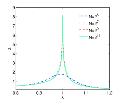
The numerical results of the RFS for a finite-size system are shown in Fig. 1, from which we can see that the peaks become sharper and sharper as the system size increases, and their locations approach to the critical point at the same time. It’s expected that there will be singular at $\lambda_{c}$ if $N$ is infinite. Then to study the scaling behavior of RFS, we define its maximum over $\lambda$ as $\chi_{m}$ with the location $\lambda_{m}$.

Figure 1: RFS as a function of $\lambda$ for various system sizes. The positions of the peaks approach to the critical point at $\lambda=1$ as increase with system sizes.

For a finite-size system, $\lambda_{m}\neq\lambda_{c}$, and yet if $N$ is large enough, $\lambda_{m}$ is so close to $\lambda_{c}$ that it’s a good approximation for us to use $\lambda_{m}=\lambda_{c}$ in computing $\chi_{m}$. The summations in Eqs. (9) and (11) converge quickly as $N$ increases, which means for large $N$, the summation can be replaced by the integral as

$$\lim_{N\rightarrow\infty}\frac{1}{N}\sum_{q=-M}^{M}\longrightarrow\frac{1}{2\pi}\int_{-\pi}^{\pi}d\phi.$$ (12)

Then it’s easy to evaluate the integrals and get

$$\langle\sigma^{z}\rangle|_{\lambda=1} =\frac{2}{\pi}, \langle\sigma_{0}^{x}\sigma_{1}^{x}\rangle|_{\lambda=1} =\frac{2}{\pi},$$

$$\langle\sigma_{0}^{y}\sigma_{1}^{y}\rangle|_{\lambda=1} =-\frac{2}{3\pi}, \langle\sigma_{0}^{z}\sigma_{1}^{z}\rangle|_{\lambda=1} =\frac{16}{3\pi^{2}}.$$ (13)

However, the first derivatives of the above quantities are divergent with respect to $N$ at $\lambda_{c}$, and we have

$$\frac{d\langle\sigma^{z}\rangle}{d\lambda}\bigg{|}_{\lambda=1} =-\frac{1}{2N}\sum_{q=-M}^{M}\left|\frac{\cos^{2}\left(\phi_{q}/2\right)}{\sin\left(\phi_{q}/2\right)}\right|\simeq-\frac{1}{\pi}\ln N,$$

$$\frac{d\langle\sigma_{0}^{x}\sigma_{1}^{x}\rangle}{d\lambda}\bigg{|}_{\lambda=1} =\frac{1}{2N}\sum_{q=-M}^{M}\left|\frac{\cos^{2}\left(\phi_{q}/2\right)}{\sin\left(\phi_{q}/2\right)}\right|\simeq\frac{1}{\pi}\ln N,$$

$$\frac{d\langle\sigma_{0}^{y}\sigma_{1}^{y}\rangle}{d\lambda}\bigg{|}_{\lambda=1} =\frac{1}{4N}\sum_{q=-M}^{M}\frac{\cos\left(2\phi_{q}\right)+\cos\phi_{q}}{\left|\sin\left(\phi_{q}/2\right)\right|}\simeq\frac{1}{\pi}\ln N.$$ (14)

The main contribution to the above expressions in the large-$N$ limit arises from the summation around the zero point of $\sin(\phi_{q}/2)$, since

$$\frac{1}{N}\sum_{q\in S}\frac{1}{\left|\phi_{q}\right|}\simeq\frac{1}{\pi}\ln N,$$ (15)

where $S$ represents the singular area. Immediately, with the help of Eqs. (4) and (11), we get

$$\frac{d\langle\sigma_{0}^{z}\sigma_{1}^{z}\rangle}{d\lambda}\bigg{|}_{\lambda=1}\simeq-\frac{16}{3\pi^{2}}\ln N.$$ (16)

The matrix elements and their derivatives could be evaluated by inserting the above results into Eq. (7). Here we should specifically consider $\partial_{\lambda}z_{-}=\partial_{\lambda}\left(\langle\sigma_{0}^{x}\sigma_{1}^{x}\rangle-\langle\sigma_{0}^{y}\sigma_{1}^{y}\rangle\right)/4$, the divergent behaviors of $\partial_{\lambda}\langle\sigma_{0}^{x}\sigma_{1}^{x}\rangle$ and $\partial_{\lambda}\langle\sigma_{0}^{y}\sigma_{1}^{y}\rangle$ at $\lambda_{c\text{ }}$are both $(\ln N)/\pi$, while their difference is convergent and could be integrated as a constant:

$$\frac{dz_{-}}{d\lambda}\bigg{|}_{\lambda=1}=\frac{1}{3\pi}.$$ (17)

Then, with Eq. (8), we get the divergent form of $\chi_{m}$ with respect to $N$ as

$$\chi_{m}\left(N\right)\simeq A_{1}\left(\ln N+c_{1}\right)^{2}+c_{2},$$ (18)

where $c_{1}$, $c_{2}$ are constants that could not be determined analytically, and the coefficient

$$A_{1} =\frac{27\pi^{4}-144\pi^{2}-1024}{\pi^{2}\left(9\pi^{2}+32\right)\left(3\pi^{2}-32\right)+4096}$$

$$\simeq 0.1485.$$ (19)

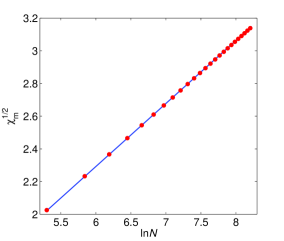
To perform a finite-size scaling analysis, we should find the logarithmic divergent quantity, and the above result suggests us to take the square root of $\chi_{m}$ for large $N$ to get the logarithmic divergent form as

$$\chi_{m}\left(N\right)^{1/2}\simeq\sqrt{A_{1}}\ln N+\text{const.}$$ (20)

Figure 2: Square of the maximum RFS over $\lambda$ as a function of $N$. The red dots are numerical results and the slope of the solid line is $\sqrt{A_{1}}$.

To confirm this, we compute $\chi_{m}^{1/2}$ numerically, and the result is shown in Fig. 2, from which we can see that the slope is excellently consistent with $\sqrt{A_{1}}$, while the linear relation is obvious for not large $N$ because $c_{2}$ is small with numerical computation. However the maximum global ground state fidelity susceptibility $S_{m}$ is of a different scaling form as $\ln S_{m}=2\ln N+$const Chen et al. (2008), thus $\ln S_{m}$ but not $S_{m}$ will exhibit similar scaling behavior with $\chi_{m}^{1/2}$ at the critical point.

III.2 Critical behavior of RFS in the thermodynamic limit

In the thermodynamic limit the total spin $N$ is infinite, then the summations can be replaced by the integrals (12) and are evaluated as:

$$\langle\sigma^{z}\rangle= \frac{1-\lambda}{\pi}\text{K}\left(k\right)+\frac{1+\lambda}{\pi}\text{E}\left(k\right),$$

$$\langle\sigma_{0}^{x}\sigma_{1}^{x}\rangle= \frac{\lambda-1}{\pi}\text{K}\left(k\right)+\frac{1+\lambda}{\pi}\text{E}\left(k\right),$$

$$\langle\sigma_{0}^{y}\sigma_{1}^{y}\rangle= \frac{1}{3\pi\lambda}\big{[}\text{K}\left(k\right)\left(\lambda-1\right)\left(2\lambda^{2}+1\right)$$

$$-\text{E}\left(k\right)\left(\lambda+1\right)\left(2\lambda^{2}-1\right)\big{]},$$ (21)

where K$\left(k\right)$ is the complete elliptic integral of the first kind and E$\left(k\right)$ is the elliptic integral of the second kind with $k=2\sqrt{\lambda}/\left(1+\lambda\right)$. Therefore the critical behavior of the RFS is determined by the elliptical integrals. At $\lambda_{c}$, we have $k_{c}=2\sqrt{\lambda_{c}}/\left(1+\lambda_{c}\right)=1$, and E$\left(1\right)=1$, while K$\left(k\right)\,$ is divergent as $k\rightarrow 1$, its asymptotic behavior is

$$\text{K}\left(k\right)\simeq\ln\frac{1}{\sqrt{1-k^{2}}}=\ln\frac{1}{\left|1-\lambda\right|},$$ (22)

from which we have K$\left(k_{c}\right)\left(1-\lambda_{c}\right)=0$. Then, obviously, at the critical point, with the above analysis we get the same results with (13) in the previous subsection.

However, their derivatives are singular at $\lambda=1$. We take $\langle\sigma^{z}\rangle$ for example,

$$\frac{d\langle\sigma^{z}\rangle}{d\lambda}=\frac{\lambda+1}{\pi\lambda}\text{E}\left(k\right)-\frac{\lambda^{2}+1}{\pi\lambda\left(\lambda+1\right)}\text{K}\left(k\right),$$ (23)

where we have used the following relations

$$\frac{d\text{K}\left(k\right)}{dk} =\frac{\text{E}\left(k\right)}{k}-\frac{\text{K}\left(k\right)}{k},$$

$$\frac{d\text{E}\left(k\right)}{dk} =\frac{\text{E}\left(k\right)}{\left(1-k^{2}\right)k}-\frac{\text{K}\left(k\right)}{k}.$$ (24)

Then as $\lambda$ approaches to $\lambda_{c}$, E$(k)$ converges quickly to 1, and with Eq. (22) we get

$$\frac{d\langle\sigma^{z}\rangle}{d\lambda}\simeq-\frac{1}{\pi}\ln\frac{1}{\left|1-\lambda\right|},$$ (25)

which is logarithmic divergent as $\lambda\rightarrow\lambda_{c}$.

Figure 3: Finite-size scaling analysis is performed. The RFS as a function of system size and coupling, collapses on a single curve for various system sizes.

The derivatives of the rest correlation functions are

$$\frac{d\langle\sigma_{0}^{x}\sigma_{1}^{x}\rangle}{d\lambda} \simeq\frac{1}{\pi}\ln\frac{1}{\left|1-\lambda\right|},$$

$$\frac{d\langle\sigma_{0}^{y}\sigma_{1}^{y}\rangle}{d\lambda} \simeq\frac{1}{\pi}\ln\frac{1}{\left|1-\lambda\right|},$$

$$\frac{d\langle\sigma_{0}^{z}\sigma_{1}^{z}\rangle}{d\lambda} \simeq-\frac{16}{3\pi^{2}}\ln\frac{1}{\left|1-\lambda\right|},$$ (26)

where the logarithmic divergent terms come from the elliptic integral K$\left(k\right)$. It’s noticed that the coefficients of the logarithmic terms are the same with those in the previous subsection for a finite-size system. Then we get a similar divergent form of $\chi$ as

$$\chi\left(\lambda\right)\simeq A_{2}\left(\ln\frac{1}{\left|1-\lambda\right|}+d_{1}\right)^{2}+d_{2},$$

where $A_{2}=A_{1}$, and $d_{1}$, $d_{2}$ are constants that could not be determined analytically.

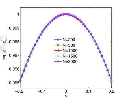
As we have derived in the above, the divergent form of the RFS around the critical point is $\left(\ln N\right)^{2}$ for finite system and $\left(\ln\left|1-\lambda\right|\right)^{2}$ in the thermodynamic limit. In order to make a finite size scaling analysis, it’s feasible for us to use the square root of the RFS, which is logarithmic divergent, and according to the scaling ansatz Barber (1983), the square root of RFS is a function of $N^{\nu}\left(\lambda-\lambda_{m}\right)$, which behaves as $\chi\left(\lambda_{m},N\right)^{1/2}-\chi\left(\lambda,N\right)^{1/2}\sim Q[N^{\nu}\left(h-h_{m}\right)]$, where $Q\left(x\right)\propto\ln\left(x\right)$ for large $x$. This function is universal and does not depend on system size $N$. Since $A_{2}=A_{1}$, we determine the scaling exponent $\nu=1$ which is the same with the concurrence Osterloh et al. (2002) and the global ground state fidelity susceptibility Chen et al. (2008), and is confirmed numerically shown in Fig. 3.

IV Conclusion

In summary, we have studied the scaling and critical behaviors of the RFS for two neighboring sites in the 1D TFIM. We found that the divergent behaviors of the RFS take the form of $\left(\ln N\right)^{2}$ for finite-size system and $\left(\ln\left|\lambda-1\right|\right)^{2}$ in the thermodynamic limit, which are distinct from other quantities like the global ground state fidelity susceptibility Chen et al. (2008), concurrence Osterloh et al. (2002) and entanglement entropy Su et al. (2006). Then we use the square root of the RFS which is logarithmic divergent to carry out a finite-size scaling analysis. The scaling exponent is determined analytically, and is confirmed numerically. It’s shown that, the RFS undergoes singularity around the critical point, thus indicate that the RFS can be used to characterize the QPTs.

V Acknowledgements

We are indebted to Shi-Jian Gu, C. P. Sun and Z. W. Zhou for fruitful and valuable discussions. The work was supported by the Program for New Century Excellent Talents in University (NCET), the NSFC with grant No. 90503003, the State Key Program for Basic Research of China with grant No. 2006CB921206, the Specialized Research Fund for the Doctoral Program of Higher Education with grant No. 20050335087.