The Cold Spot as a Large Void:
Rees-Sciama effect on CMB Power Spectrum and Bispectrum
Abstract
Abstract
The detection of a “Cold Spot” in the CMB sky could be explained by the presence of an anomalously large spherical underdense region (with radius of a few hundreds ) located between us and the Last Scattering Surface. Modeling such an underdensity with an LTB metric, we investigate whether it could produce significant signals on the CMB power spectrum and bispectrum, via the Rees-Sciama effect. We find that this leads to a bump on the power spectrum, that corresponds to an correction at multipoles ; in the cosmological fits, this would modify the by an amount of order unity. We also find that the signal should be visible in the bispectrum coefficients with a signal-to-noise , localized at . Such a signal would lead to an overestimation of the primordial by an amount for WMAP and by for Planck.
pacs:
98.80.Cq, 98.80.Es, 98.65.Dx, 90.70.VcI Introduction
The recent WMAP WMAP experiment has measured with great accuracy the anisotropies of the Cosmic Microwave Background (CMB), whose features are in good agreement with the expectations from inflation of a Gaussian spectrum of adiabatic fluctuations, fully described by a nearly scale-invariant power spectrum. However, it has been pointed out by several authors that the data contain various unexpected features. Some of them are localized at very large angular scales, such as the low quadrupole, the alignment of the low multipoles (for a review see reviewlowl and references therein) and the power asymmetry between the northern and southern hemispheres hemispherical . Another anomaly is the presence of the so-called Cold Spot ColdSpot1 ; ColdSpot2 ; ColdSpot3 , which is a large circular region on an angular scale of about that appears to be anomalously cold: the probability that such a pattern would appear from Gaussian primordial fluctuations is estimated to be about ColdSpot1 ; ColdSpot2 ; ColdSpot3 . So, while this could still be a statistical fluke, some authors have put forward the idea that it could instead be due to an anomalously large spherical underdense region of some unknown origin, on the line of sight between us and the Last Scattering Surface (LSS) Tomita ; InoueSilk . We may also remind that rudnick has claimed that, looking at the direction of the Cold Spot in the Extragalactic Radio Sources (the NVSS survey), an underdense region is visible at redshift (see, however huterer for a paper that challenges this claim). Another motivation for studying such objects is that an underdense region of two or three hundreds of could be enough to give an acceptable fit to the Supernova data and the CMB without Dark Energy ABNV , if we happen to live near its centre.
In this paper we also take the point of view that the Cold Spot could be due to such an underdense region, customarily denoted as a “Void”. By modeling it through an inhomogeneous Lemaître-Tolman-Bondi (LTB) metric (which also requires an overdense compensating shell), we compute the impact of such a Void on some observational quantities, focusing on the statistical properties of the CMB: in particular on the two-point correlation function (power spectrum) and the three-point correlation function (the bispectrum). This is interesting for the following reasons. First, if there is such a Void, does the power spectrum get a sizable correction? And, if yes, to what extent the estimation of the cosmological parameters is affected? Second, if there is such a Void, could it be detectable also in the bispectrum? Third, does the presence of such an object interfere with the measurement of a primordial non-gaussianity, which constitutes a very important piece of information in order to distinguish between models of inflation?
It is well known that, passing through a Void, photons suffer some blue-shift due to the fact that the gravitational potential is not exactly constant in time – the so-called Rees-Sciama (RS) effect ReesSciama . By RS effect we mean the one associated to the variation of the gravitational potential from non-linear effects. There can be an effect already at the linear level, usually referred to as the Integrated Sachs-Wolfe (ISW) effect, which however would vanish in a matter dominated flat Universe. The ISW effect would be significant only when a Dark Energy component becomes dominant with respect to matter. Hence, here we focus our attention only on the RS effect, which is always present, and briefly comment on the extension to a CDM Universe later on. Note that there is a second physical effect due to a Void on the line of sight, in addition to the RS blue-shift of the photons: the lensing of the primordial perturbations, which will be analyzed in detail in a companion paper LENS .
It is also known that the RS effect scales as the third power of the comoving radius of the Void times the present value of the Hubble parameter , . For Void sizes compatible with the expectations from the usual structure formation scenarios, the RS effect happens to be suppressed with respect to the primordial temperature fluctuations Fullana . In order to produce a signal comparable to the measured temperature anisotropy of , the Void should be of very large size, i.e. : this would be at odds with the standard scenario of structure formation from Gaussian primordial fluctuations (at more than InoueSilk ). We may also mention that according to manyvoids ; Szapudi there are many localized regions in the sky (both underdense and overdense) of about , which would be responsible for the correlations between the CMB and the Large Scale Structures: as SarkarVoids has recently stressed the existence of these regions is already at odds with the usual structure formation scenario. Even though we do not address in this paper the issue of the primordial origin of such large objects, we mention some possibilities. For example, one could consider certain models of inflation, such as the ones of the “extended” type extended ; extendedDMN ; extendedBN , with the possibility of tunneling events and nucleation of bubbles, which would appear as Voids in the sky today. Alternatively, one could also imagine the presence of non-Gaussian features in the primordial fluctuations which would seed a large Void or even non-conventional structure formation histories in the late-time Universe which could enhance the probability of having large Voids.
In the case of an explanation of the Voids via tunneling events, it is interesting to note that if a nucleation process has small probability (per unit volume and time) compared to the Hubble rate (at some time during inflation) then the number of anomalous Voids could well be very small, such as having just one or a few of them in the present observable Universe. In addition, since the LSS is a rather thin shell whose volume is much smaller than the total volume inside it, if there are only few Voids it is more likely that they are located along the line of sight, rather than at the LSS111It is possible, also, to imagine that some primordial process could generate a coherent spherical region on the LSS surface, with small density contrast, on top of the primordial Gaussian spectrum, and which would produce a fluctuation. However, we do not consider here such possibilities.. This is an important point because a Void at the LSS would have a huge impact on the CMB and, as a consequence, its size would be strongly constrained: emptyVoids ; extendedDMN . On the contrary, Voids on the line of sight are not subject to the latter constraint.
Note also that other authors have put forward alternative ideas, such as the idea that the Cold Spot could be due to a topological defect, in particular a cosmic texture texture . As we are going to discuss, some of our considerations apply in a similar fashion if the origin of the Cold Spot is a texture, rather than a Void.
The paper is organized as follows. In sect. II we calculate the RS-induced temperature profile of the CMB photons passing through a large Void with the physical characteristics of the Cold Spot. The impact on the power spectrum is discussed in sect. III, while sect. IV deals with the impact on the bispectrum and on the overestimation of that would be done by neglecting the presence of such a Void. Finally, in sect. V we extend some of the considerations to the case of several objects in the sky. In fact, it is conceivable that if there is one such structure, there may be other ones, maybe of smaller size and less visible – see e.g. manyvoids ; Szapudi for some other candidates in the CMB sky. Our conclusions are drawn in sect. VI.
II A Void in the line of sight
As anticipated in the introduction, we would like to consider the following cosmological configuration: an observer looking at the CMB through one spherical Void located at comoving distance from him. We assume that the object does not intersect the LSS and that the observer is not inside it. The observer receives from the LSS the CMB photons, whose fluctuations we assume to be adiabatic, nearly scale-invariant and Gaussian (as those generated e.g. by the usual inflationary mechanism). Given this configuration, the observer detects one particular realization of the primordial inflation-generated perturbations on the LSS plus the secondary effects due to this anomalous structure located in the line of sight. Our aim is to give the theoretical prediction for the two-point and three-point correlation functions, in order to compare them with the observations.
As a first step we consider that the Universe and the LSS are just completely homogeneous, and study what kind of profile we should see in the sky, because of the existence of one inhomogeneous Void located between us and the LSS: we denote the temperature fluctuation obtained in this way as , where (RS) stands for Rees-Sciama. As a second step, we consider that there are Primordial fluctuations present on the LSS that will also be affected by the presence of the Void: in fact, they will be lensed by it, leading to an additional effect, . So, finally, the total temperature fluctuation will be given by:
| (1) |
where by definition each -labeled fluctuation is given by
| (2) |
with the bar representing the angular average over the sky and .
At this point it is important to be more precise about the origin of the Void, relatively to the Primordial fluctuations. If such a structure comes from the same physical process as the Primordial Gaussian spectrum, then this would mean that there is some correlation between the two. However we will assume, from now on, that the location of the Void in the sky is not correlated at all with the Primordial temperature fluctuations coming from inflation. This is true, for example, if such structures come from a different process, such as nucleation of bubbles. Note that this is a conservative assumption since, in the presence of a correlation, the temperature correlation functions would be generically enhanced.
Then, we need to fix the properties of the Void in order to compute the RS (and Lensing) contributions. Physically, one may characterize such a Void via the following quantities: its comoving distance from us, its comoving radius , its present-day density contrast at the centre , and some shape for the density profile. As we will discuss, the RS fluctuation turns out to be described by two parameters: its amplitude at the centre and its angular extension, characterized by the diameter of the Cold region. We also need some shape for the temperature profile, which will be determined by choosing some shape for the density profile of the Void. Let us discuss in more detail how the parameters and are related to the physical parameters of the Void, namely : the amplitude mostly depends on the radius and the density contrast , while it is is not very sensitive to ; the diameter depends on the ratio . As explained in the next paragraph, we choose the values for and phenomenologically. Clearly this leaves a degeneracy in the choice of the physical parameters, since we have three of them (, and ) and only two observational constraints ( and ).
In order to fix a range for the amplitude we rely on the values given by texture as follows. The minimal temperature in real space observed in the Cold Spot area is ColdSpot1 , but this value includes as well a contribution from the Primordial Gaussian profile, . The authors of ColdSpot1 use a temperature profile for the secondary effect, add the Gaussian fluctuation and fit the observational data: this leads to an estimation for the value of the secondary effect at the centre, given by , or equivalently . In this paper we assume the latter range of values for . This is probably not entirely accurate (the shape of the profile that we use is slightly different from theirs, since we consider a compensated Void, while the profile in texture corresponds to the profile due to a cosmic texture), but it should give a good estimate for the range of values of interest. In any case, our results can be easily rescaled for different values of . As for the angular size of the profile, we proceed as follows. According to ColdSpot2 ; ColdSpot3 , a shape that fits well the Cold Spot has a diameter of about for the very cold part, but we also show in all plots the extreme case : in fact as one can see in fig.1 of ColdSpot3 the entire cold region extends up to such large size.
Having fixed the numerical values, we choose a metric to model such an inhomogeneous region. The choice that we make is a spherically symmetric LTB metric, which is matched to a homogeneous and isotropic Friedman-Lemaître-Robertson-Walker (FLRW) flat model. For simplicity we consider a flat FLRW Universe with . Including a dark energy component would lead to an ISW effect already at the linear level, in addition to the RS effect that we consider, which is present in any case, even in absence of dark energy. The effect of a cosmological constant in an analogous setup has been studied e.g. by InoueSilk ; SakaiInoue and the two effects turn out to be similar, with the same dependence on the Void radius, but with some difference on the dependence on the density contrast 222Specifically, the dependence is different in the presence of : the second-order term (RS effect) is suppressed, but there is a non-zero linear term. For small density contrast, , the linear ISW would dominate in a -dominated cosmology. The quadratic term dominates if is large or if is close to 1. An interesting case is the one for intermediate values (): the two effects are roughly compensating and the calculation does not depend much on the value of ..
Another important point is that our profile is a compensated Void, with the underdense central region surrounded by a thinner external overdense region. This is a requirement dictated by the matching conditions, which corresponds to the condition that the Void does not distort the outer FLRW metric. Physically, if the Void comes e.g. from a primordial bubble of true vacuum, this is a consistent requirement: in fact a bubble would have a thin wall with localized gradient energy, compensating for the lower energy contained in the true vacuum in the interior region. Note that, because of this feature, the angular size of the entire LTB patch that we consider will be larger than , since we have a hot region as well. In any case, we show that the main contribution to the power-spectrum and bispectrum comes from the inner underdense region.
Given these specifications for we now compute its shape in the following subsections.
II.1 Temperature Profile
First of all, we model the profile as an LTB metric with irrotational dust, which describes a compensated Void. It has been shown in BN that this metric can be treated, in some cases, as a perturbation of an FLRW metric with a gravitational potential given by the following (Newtonian gauge) expression
| (3) |
where is the conformal time and are dimensionless comoving coordinates. We have chosen units such that the present value of the conformal time is . As a function of the dimensionless comoving radial coordinate , the gravitational potential is given by:
| (4) |
where is an arbitrary function which represents the local curvature and determines the shape of the density profile. This approximation is valid as long as is small. The only constraints on this function comes from the smoothness of the density profile at the centre (which dictates , where the prime denotes a derivative with respect to the coordinate) and from the requirement that the LTB patch matches to a flat FLRW universe (). We have chosen arbitrarily the function as follows:
| (5) |
where , is the dimensionless radius of the LTB patch and is the present value of the Hubble parameter. The density contrast that results from the choice of is approximately given by the following expression BN :
| (6) |
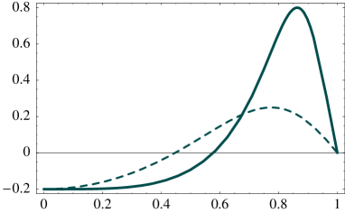
where is the matter energy density inside the LTB patch, is the average density in the outer FLRW region. Note that the density contrast can be large even if is small. We show in fig. 1 the density profiles corresponding to certain values of . From (5) and (6) it follows that the value of the normalization constant is directly related to (the value of the present day density contrast at the centre of the Void): .
|
Given the potential we can compute the for a photon which travels through this patch, by computing a line integral, following the expression given in MM ; BMM which is valid at second order in perturbation theory in :
| (7) |
where is the value of the conformal time at emission (although of course the integrand is nonzero only in the region where the LTB structure is located). The conformal time evolves simply as , where the subscript refers to the observer space-time point. Here is a non-local quantity, which is given in terms of as BMM ; BN :
| (8) |
Then, using the spherical coordinates angles, and , we may parameterize the temperature profile as
| (9) |
where the profile function is normalized so that . The profile has no dependence on because we choose the axis to point towards the centre of the Void. The factor can be computed performing the integral (7) analytically along a radial trajectory, and it is a function of the physical parameters of the configuration: the radius of the LTB patch, the density contrast at the centre of the Void and the distance between the observer and the centre of the Void. The result is333The dependence on the shape of the density profile (the parameter) comes in the numerical factor and it is given by , which ranges between 0.05 and 1.85. This variability in the prefactor could account for the prefactors obtained by previous analyses InoueSilk ; SakaiInoue , which are of about ., at leading order in ,
| (10) |
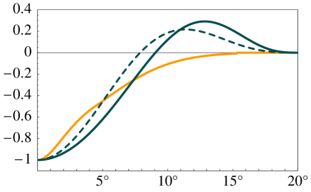
Note that the dependence on the distance is a weak correction, unless the patch happens to be located at distances comparable to the horizon. We can compute the function by numerical integration of (7) along a non-radial trajectory (computed as an unperturbed straight line, since any deviation would lead only to higher order corrections). In fig. 2 we plot the profile as a function of for two values of . For the reader’s convenience, we provide polynomial interpolations of the profiles:
where . We have added also a light solid line in fig. 2 which shows, for comparison, the temperature profile of the cosmic texture that provides the best fit to the Cold Spot, as discussed in texture (its profile has also been normalized so that at the centre). Notice that the compensated Void has a hot ring in the profile, while the texture does not have it 444There is one caveat, however: in a dominated cosmology and with small contrast , the linear ISW can become the dominant effect; and it has been shown by InoueSilk that this case does not lead to a hot ring..
|
II.2 Decomposition into spherical harmonics
The spherical harmonic decomposition of the -th profile for the temperature anisotropy of (1) is defined as:
| (12) |
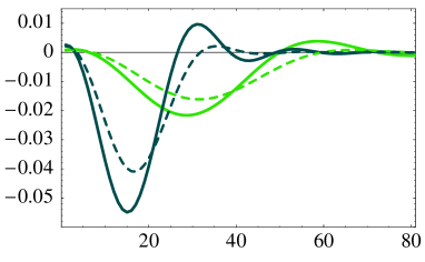
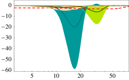
For the (RS) component, since the profile is symmetric with respect to the axis pointing towards the centre of the Void, only the coefficients with are non-vanishing (and they are real). In the left plot of fig. 3 we show the ratio as a function of the multipole . The dark solid (dashed) curve corresponds to a temperature profile with and (), hence to a Cold Spot with diameter (); the light solid (dashed) curve is obtained by choosing instead , so that (). Notice that the medium amplitude of such a ratio is roughly equal to the fraction of the sky covered by our LTB patch, namely about for and for , respectively concentrated at multipoles and .
One may wonder whether the presence of a compensating hot shell (see fig. 2) in our profile has a significant impact on the magnitude and shape of the coefficients. As an example, in the right plot of fig. 3 we focus on the with and (solid line), and show how they would change by truncating the temperature profile only to the cold part (dashed line). This approximately mimics a truncation of the density profile only to the underdense region (the true Void), disregarding the overdense compensating shell. One can see that the are now suppressed but still quite similar, so that for our purposes the result is not going to be very different. This shows that the RS effect mainly comes from the underdense region. The same plot also shows, for comparison, the ratio that one would obtain from the temperature profile of the texture giving the best fit to the Cold Spot texture . Notice that the texture and the non-compensated Void are pretty similar.
|
III Power spectrum
Given a temperature profile with its coefficients one can compute the associated two-point correlation function. In general, given a single set of coefficients, the two-point correlation function (power spectrum) is defined via the ’s coefficients as
| (13) |
Note that this definition ensures that the ’s do not depend on the choice of the coordinate system on the sphere. Therefore we are free to keep our axis aligned with the centre of the Void. In our case and, in order to face it with the experimentally observed value of , we have to estimate the theoretical prediction for , where the brackets stand for a statistical average over an ensemble of possible realizations of the Universe – or, equivalently, an average over many distant uncorrelated observers.
For a Primordial and Gaussian signal the two-point correlation functions are given by:
| (14) |
where the are predicted by some mechanism (i.e. inflation) that can generate Primordial
Gaussian fluctuations.
Then, there are two types of effects on the power spectrum due to our secondary effects:
i) the inflationary prediction receives corrections;
ii) there is also some non-diagonal correlation between different ’s.
As we have already stressed, we assume that the Rees-Sciama (RS) component in (1) is uncorrelated with the Primordial (P) component, which means that it can be factored out of the brackets. Given this fact, from (1) and (12), we get two types of non-zero contributions for : the RS-RS contribution proportional to , and the P-L contribution proportional to . The first effect is computed in the next subsection, while the second in the companion paper LENS .
III.1 Rees-Sciama power spectrum
As we have seen, for a spherical Void in the -direction, if . Hence the RS contribution to the power spectrum coefficients, , is just:
| (15) |
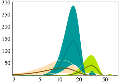
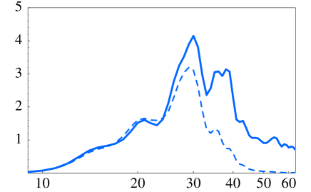
In the left and right panels of fig. 4 we have plotted respectively the quantities and , for the range of parameters mentioned in sect. II. The shaded regions are indeed obtained varying the amplitude in its - range, namely . The results for different values of can be extracted just by noticing that . As one can see, for a Void with a size which can account for the Cold Spot, the correction to the power spectrum is non-zero only in the range and its magnitude is about with respect to the Primordial signal. We also note that the RS correction is of the order of the cosmic variance, . For comparison, we also show in the left panel of fig. 4 the correction to the power spectrum obtained from the texture of texture , which turns out to be smaller and shifted at lower multipoles with respect to the Void case.
|
In order to see how large is the impact on the cosmological parameter estimation due the RS effect from a large Void, one should perform a detailed statistical analysis of the CMB data, which we postpone for future work HMN . For the purpose of this paper, we may just estimate the impact that the inclusion of the RS effect has on the of the fit, which gets increased by the amount:
| (16) |
where is the variance of the two-point correlation function, including the cosmic variance and the instrumental noise. For an experiment like WMAP, the cosmic variance is the dominant source of error at low-’s, so that we can just neglect the instrumental noise and use . The sum gives roughly the following result, for different angular diameters of the Void:
| (17) |
Finally, as already mentioned, there is also a non-diagonal contribution to the two-point correlation function, which correlates different ’s in the range and is of the same order of magnitude as the diagonal contribution to the power spectrum, .
IV Bispectrum
Having computed the coefficients and the two-point correlation functions, we now estimate the impact that a large Void has on the bispectrum coefficients, also to check whether this observable could be used to constrain the size and the density of the Void itself, which is a highly non-Gaussian object. Moreover, since the bispectrum is the main tool used to make detections of a primordial non-gaussianity, it is interesting to see whether the presence of a large Void can contaminate this detection and to what extent.
Note that the bispectrum from the the RS effect due to conventional structures, i.e. with non-linearities at scales of order , has already been studied by several authors SpergelGoldberg ; MatarreseRS . However, the calculation here is quite different for two reasons: i) we deal with much larger values for the ’s, because we consider larger values of and the RS effect on the temperature profile is proportional to ; ii) we are assuming no correlations between the RS and the Primordial fluctuations, while this is not the case in the conventional calculation where the RS effect arises from the structures seeded by the Primordial fluctuations themselves. In addition, we compute in LENS the associated Lensing effect.
The basic quantities are now the coefficients, defined as
| (18) |
which are coordinate-dependent quantities. So, in analogy with the ’s coefficients, one introduces the angularly averaged bispectrum
| (19) |
where the matrix represents the Wigner 3-j symbols and the sum is carried over all possible values for the ’s. One can indeed show, by using the properties of the Wigner 3-j symbols review , that this combination does not depend on the chosen -axis, so that these quantities are more suitable to make predictions. For convenience, we nevertheless keep our -axis along the direction of the centre of the Void.
We are thus interested in evaluating and, using (1) and (19), one realizes that it corresponds to a sum of 27 terms, of which 23 have zero statistical average. As already mentioned, a crucial assumption that we make here is that the coefficients are not stochastic quantities, which means that the location of the Void in the sky is not correlated at all with the Primordial temperature fluctuations coming from inflation (this is a conservative assumption: if there is some correlation, the non-gaussianity could be much more important, since some terms would be non-zero). Under this assumption, the four types of terms that potentially survive are the ones involving: , , and . However, as shown in Appendix A, the potentially very large terms are actually exactly zero (because of the absence of correlations between RS and P). Moreover, since , we can neglect the terms with respect to the terms.
Summarizing, we are left with two types of contributions to :
| (20) |
| (21) |
We compute the first one in the following subsection, while the second in LENS .
IV.1 Non-gaussianity from RS effect
To compute the term is very simple. The only non-zero coefficients are those with , so that:
| (22) |
It is customary to define a reduced bispectrum via the following:
| (23) |
|
We plot the diagonal contribution in fig. 5: the equivalent amplitude is very high compared to a typical primordial signal, since it corresponds roughly to . However, for the RS signal due to the large Void goes rapidly to zero. Therefore, for experiments like WMAP or Planck, which go up to about and respectively, only a small subset of the data is affected by the RS contribution.
Focusing on the RS signal, we now turn to estimate whether it is detectable or not. The signal on a single multipole is lower than the cosmic variance: so we have to sum over all the ’s to find a bispectrum Signal-to-Noise () ratio. For a signal labeled by , this is defined as (see e.g. review ):
| (24) |
where is the variance of the bispectrum:
| (25) |
and or respectively if all ’s are different, if only two of them are equal or if they are all equal. The ’s represent the sum of the CMB power spectrum plus the power spectrum of the noise of the detector. In general, at some the noise becomes dominant, while below the variance is dominated by the Primordial one, namely .
|
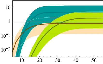
Neglecting the instrumental noise, in the left panel of fig. 6 we show the result for as a function of . As one can see, the signal is detectable for a large part of the parameter space: so it should already be possible to look for such a signal in the WMAP data. Conversely, the absence of any detection would give interesting constraints on the size and density of a large Void. We show in the right panel of fig. 6 the region of physical parameter space which would give rise to a detectable signal, namely : for a cold region diameter , this happens for all the points in the light shaded region. For such region gets larger and includes the dark shaded one. For instance, for a Void with and , a signal in the bispectrum would appear only if , which corresponds to .
IV.2 Contamination of measurements
We now turn to the impact that a huge Void in the line of sight would have on the measurement of the primordial non-gaussianity parameter , in terms of which it is customary to parametrize a primordial non-Gaussian signal. By definition, is introduced (see e.g. review for details) parameterizing the primordial curvature perturbations as follows:
| (26) |
where is the linear Gaussian part of the perturbation. Given a physical model (like slow-roll inflation) is generically a function of the momenta, i.e. , but in the quantitative data analyses it is usually assumed to be just a constant number. Note that single field minimally coupled slow-roll inflationary models predict very small values for , that is Maldacena ; Acquaviva , but other models may predict larger values (see e.g. review ). The primordial bispectrum coefficients can be written as:
| (27) |
where the have a specific form in terms of the primordial spectrum and the radiation transfer function.
As we have seen, the RS effect leads to a large contribution to for multipoles in the range . On the contrary, the Lensing effect LENS is much smaller at low ’s, but could contaminate the primordial bispectrum signal at large ’s, since it couples the low RS-’s with the high ’s of the primordial signal LENS . The impact on due to the RS effect can be computed by estimating the following ratio review ; cooray :
| (28) |
In other words, if a large Void exists, one should subtract it from the data in order to get the correct value for , thus avoiding to overestimate the latter by the amount .
We may very easily give an approximation of the appearing in the numerator of (28) by using (23) with the Sachs-Wolfe approximation for the primordial signal:
| (29) |
This is a good approximation only for the low- plateau in the power spectrum, while the full expression should be used for higher ’s. However, since vanishes if any of the ’s is larger than about , we consider it to be a sufficiently fair approximation to get an estimate of the numerator of (28). This fact also allows to neglect the experimental noise in the numerator’s . Instead the denominator is a quantity very sensitive to the experiment (see review ). In fact, at some high (dependent on the experiment) the experimental noise in the of the denominator becomes so large that the multipoles give a negligible contribution to the sum. Accordingly, the denominator of (28) turns out to be equal to for WMAP () and for Planck () review , so that one obtains:
| (30) |
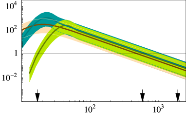
It is also interesting to study the dependency of for smaller values of . This can be easily done because the denominator in (28) is well approximated by Komatsu:2001rj , until the experimental noise is negligible. The result is plotted in fig. 7: from the left panel it turns out that the RS effect due to the large Void does not affect much the measurements for high resolution experiments. In fact, the corrections are localized at low ’s because get a sizable RS correction only if , while the search for a primordial non-gaussianity uses all the experimental data-points up to . Therefore, even if the multipoles are strongly affected, they only represent a small fraction of all the bispectrum data-points. Note also that the impact on is roughly the same for and : the reason is indeed that a smaller Void affects higher ’s, which are more relevant for the extraction of the primordial .
|
The right plot in fig. 7 allows a direct comparison with the WMAP-1year experimental constraints on WMAP1GAUSS . We can already see that some region of the parameter space can be excluded for the Void with : values for the amplitude are excluded at - by the error bar localized at . Of course, such an analysis would require a more refined technical treatment – for example including the recent WMAP 5-year data, sky-cuts, the full expression for – which we do not address in the present paper. A full analysis should also include the correlation matrix with other cosmological sources: SZ-lensing effect, point sources and the primordial signal. Anyway, looking for is not the best way to constrain a large Void: one should rather compare directly the observed bispectrum data with the prediction for . Since we have shown in fig. 6 that the RS Signal-to-Noise is above unity for most of the parameter space, a full analysis should be able to set interesting constraints.
Finally, we may also give a comment on the results by Yadav , whose authors claim a detection of primordial non-gaussianity already in the WMAP data. In their analysis they also find that, masking the region which corresponds to the Cold Spot, their measured goes up by an amount of . In the light of our analysis, this cannot be due to the RS effect, because the RS contribution to is smaller (about ) for WMAP and, moreover, has opposite sign. The possibility that this could be ascribed to the Lensing effect will be discussed in LENS .
V Other Voids
We briefly comment in this section about the possibility that several Void regions are present in the sky. The authors of manyvoids ; Szapudi have claimed detection of the ISW effect because it could explain the correlations that they were able to identify between the galaxy surveys and the CMB data. By exploring a region of the northern hemisphere that covers about of the sky, Szapudi has catalogued about 50 of such Voids555The Cold Spot, located in the southern hemisphere, is clearly not among them., which have a mean radius of about and a mean amplitude (or, equivalently, K); their density contrast for the luminous matter can be directly observed in the galaxy surveys; the knowledge of their redshift also allows to estimate their physical size , which turns out to be of about . As stressed in the introduction, SarkarVoids has interestingly pointed out that the existence of such large Voids is unlikely to be explained by the standard structure formation scenario. It could be relevant, therefore, to apply our considerations to these Voids as well.
If Voids are present in the sky, however, there are differences with respect to the analysis developed in the previous sections. If we focus on the two-point correlation function, in addition to the terms of the same type as (15), we have to compute also interference terms. As for the three-point correlation function, it would contain terms of the same kind as (22), plus interference terms. For a random distribution of Voids in the sky, one expects the interference terms to add up incoherently, leading only to an oscillatory modulation of the correlation functions.
For a precise computation of the effect of these Voids on the power spectrum and bispectrum, it would be necessary to know, for each Void, its location, the amplitude and the angular size of its temperature profile. Note that the most of the contribution is expected to come from the few Voids with the largest and . The authors of Szapudi give these informations for the 50 Voids identified, except for the amplitude , for which only the mean value is provided.
We can nevertheless give an estimate of the impact on the CMB due to the RS effect of the Voids catalogued in Szapudi (their location is sketched in the right panel of fig. 8), by assigning to each of them an amplitude equal to the mean one. The angular size of the Voids spans from to , and there are 19 Voids with . The left panel of fig. 8 shows the result for the two-point correlation function (where we also show that the interference terms are negligible), whose order of magnitude can be understood by the following easy argument. Rescaling to the case of an amplitude the results obtained in sect. III for one Void with radius of about , one gets: . Assuming that the interference terms (which depend on the relative location in the sky of the Voids) are irrelevant, the latter value for a single Void has to be multiplied by , thus obtaining , consistently with the left plot of fig. 8. We may estimate the contribution to the three point function similarly. The signal-to-noise ratio for a Void of radius and amplitude would be of about , as shown in sect. IV. As done before, the final result is obtained by multiplying by the number of Voids, leading to , assuming again that the interference terms are negligible.
|
VI Conclusions
Motivated by the so-called Cold Spot in the WMAP data, we have studied in this paper the impact on statistical CMB predictions, in particular the two and three point correlation functions, of the presence of an anomalously large Void along the line of sight. Indeed, the existence of such a Void could be at the origin of the Cold Spot, due to the Rees-Sciama effect (the Lensing effect is analyzed in the companion paper LENS ).
First, we have computed the temperature profile using an LTB solution of the Einstein equations, matched to an FLRW metric. Then, we have computed its impact on statistical predictions for the CMB, assuming this structure to be uncorrelated with the Primordial fluctuations. As suggested by texture , we consider the angular size of such a Void to be about and its temperature at the centre to be characterized by .
For the power spectrum the results are as follows. The RS effect is non-negligible: we predict a bump of to be added to the Primordial spectrum, localized at multipoles . This should lead to a variation in the for the WMAP fits of order unity.
Then we have studied the impact on the bispectrum coefficients. For the RS effect we have found that the Signal-to-Noise ratio is larger than unity at for most of the parameter space, and therefore this should already be visible in the available data. Through the bispectrum, we have studied also the impact of such a structure on the determination of the primordial non-gaussianity. The RS bispectrum signal is large but localized at low multipoles (), so it has a small impact on high resolution experiments, which can go up to very large multipoles: the overestimation of due to the RS effect turns out to be for WMAP and for Planck. Using the already existing WMAP1-year constraints WMAP1GAUSS on at low , one can exclude extreme values of the temperature contrast of the Void. For example, values for larger than for a Cold Spot with diameter of are likely to be excluded, via a full analysis. So, we conclude that the bispectrum is a valuable tool for constraining an anomalously large Void, through the RS effect.
We have also considered the 50 Voids whose detection has been claimed in Szapudi . These Voids have mean angular diameter of about and average temperature at the centre characterized by . The effect on the two-point correlation function is about , hence much smaller than the one due to the large Void considered to explain the Cold Spot. The effect on the three-point correlation function has not been studied in detail but it is expected to lead to a Signal-to-Noise ratio smaller than one.
Finally, we have also applied our considerations to the case in which the Cold Spot is explained by a cosmic texture texture rather than a large Void: the effect on the power spectrum is similar but somewhat smaller; the three-point correlation function leads also to a smaller Signal-to-Noise ratio, which however turns out to be above unity for some part of the parameter space.
Acknowledgements.
We would like to thank Tirtho Biswas, Marcos Cruz, Paul Hunt, Bob McElrath, Oystein Rudjord and Subir Sarkar for useful discussions and suggestions.References
- (1) G. Hinshaw et al. [WMAP Collaboration], arXiv:0803.0732 [astro-ph].
- (2) D. Huterer, New Astron. Rev. 50, 868 (2006) [arXiv:astro-ph/0608318].
- (3) H. K. Eriksen, F. K. Hansen, A. J. Banday, K. M. Gorski and P. B. Lilje, Astrophys. J. 605, 14 (2004) [Erratum-ibid. 609, 1198 (2004)] [arXiv:astro-ph/0307507]; H. K. Eriksen, A. J. Banday, K. M. Gorski, F. K. Hansen and P. B. Lilje, Astrophys. J. 660, L81 (2007) [arXiv:astro-ph/0701089].
- (4) M. Cruz, E. Martinez-Gonzalez, P. Vielva and L. Cayon, Mon. Not. Roy. Astron. Soc. 356, 29 (2005) [arXiv:astro-ph/0405341].
- (5) M. Cruz, M. Tucci, E. Martinez-Gonzalez and P. Vielva, Mon. Not. Roy. Astron. Soc. 369, 57 (2006) [arXiv:astro-ph/0601427].
- (6) M. Cruz, L. Cayon, E. Martinez-Gonzalez, P. Vielva and J. Jin, Astrophys. J. 655, 11 (2007) [arXiv:astro-ph/0603859].
- (7) K. Tomita, Phys. Rev. D 72, 103506 (2005) [Erratum-ibid. D 73, 029901 (2006)] [arXiv:astro-ph/0509518].
- (8) K. T. Inoue and J. Silk, Astrophys. J. 648, 23 (2006) [arXiv:astro-ph/0602478]; K. T. Inoue and J. Silk, Astrophys. J. 664, 650 (2007) [arXiv:astro-ph/0612347].
- (9) N. Sakai and K. T. Inoue, arXiv:0805.3446 [astro-ph].
- (10) L. Rudnick, S. Brown and L. R. Williams, arXiv:0704.0908 [astro-ph].
- (11) K. M. Smith and D. Huterer, arXiv:0805.2751 [astro-ph].
- (12) S. Alexander, T. Biswas, A. Notari and D. Vaid, arXiv:0712.0370 [astro-ph].
- (13) M. J. Rees and D. W. Sciama, Nature 217, 511 (1968).
- (14) I. Masina and A. Notari, in preparation.
- (15) N. Puchades, M. J. Fullana, J. V. Arnau and D. Saez, Mon. Not. Roy. Astron. Soc. 370, 1849 (2006) [arXiv:astro-ph/0605704]; U. Seljak, arXiv:astro-ph/9506048; N. Sakai, N. Sugiyama and J. Yokoyama, Astrophys. J. 510, 1 (1999) [arXiv:astro-ph/9712153].
- (16) J. D. McEwen, P. Vielva, M. P. Hobson, E. Martinez-Gonzalez and A. N. Lasenby, Mon. Not. Roy. Astron. Soc. 373 (2007) 1211 [arXiv:astro-ph/0602398]; P. D. Naselsky, P. R. Christensen, P. Coles, O. Verkhodanov, D. Novikov and J. Kim, arXiv:0712.1118 [astro-ph].
- (17) B. R. Granett, M. C. Neyrinck and I. Szapudi, arXiv:0805.2974 [astro-ph]; B. R. Granett, M. C. Neyrinck and I. Szapudi, arXiv:0805.3695 [astro-ph].
- (18) P. Hunt and S. Sarkar, arXiv:0807.4508 [astro-ph].
- (19) C. Mathiazhagan and V. B. Johri, Class. Quant. Grav. 1, L29 (1984); D. La and P. J. Steinhardt, Phys. Rev. Lett. 62, 376 (1989) [Erratum-ibid. 62, 1066 (1989)]; Phys. Lett. B 220, 375 (1989).
- (20) F. Di Marco and A. Notari, Phys. Rev. D 73, 063514 (2006) [arXiv:astro-ph/0511396]
- (21) T. Biswas and A. Notari, Phys. Rev. D 74, 043508 (2006) [arXiv:hep-ph/0511207].
- (22) A. R. Liddle and D. Wands, Mon. Not. Roy. Astron. Soc. 253, 637 (1991).
- (23) M. Cruz, N. Turok, P. Vielva, E. Martinez-Gonzalez and M. Hobson, Science 318, 1612 (2007) [arXiv:0710.5737 [astro-ph]];M. Cruz, E. Martinez-Gonzalez, P. Vielva, J. M. Diego, M. Hobson and N. Turok, arXiv:0804.2904 [astro-ph].
- (24) T. Biswas and A. Notari, JCAP 0806, 021 (2008) [arXiv:astro-ph/0702555]; T. Biswas, R. Mansouri and A. Notari, JCAP 0712, 017 (2007) [arXiv:astro-ph/0606703].
- (25) S. Mollerach and S. Matarrese, Phys. Rev. D 56, 4494 (1997) [arXiv:astro-ph/9702234].
- (26) S. Matarrese, S. Mollerach and M. Bruni, Phys. Rev. D 58, 043504 (1998) [arXiv:astro-ph/9707278].
- (27) P. Hunt, I. Masina and A. Notari, in preparation.
- (28) S. Mollerach, A. Gangui, F. Lucchin and S. Matarrese, Astrophys. J. 453 (1995) 1 [arXiv:astro-ph/9503115].
- (29) D. N. Spergel and D. M. Goldberg, Phys. Rev. D 59 (1999) 103001 [arXiv:astro-ph/9811252]; D. M. Goldberg and D. N. Spergel, Phys. Rev. D 59 (1999) 103002 [arXiv:astro-ph/9811251].
- (30) N. Bartolo, E. Komatsu, S. Matarrese and A. Riotto, Phys. Rept. 402, 103 (2004) [arXiv:astro-ph/0406398].
- (31) J. M. Maldacena, JHEP 0305, 013 (2003) [arXiv:astro-ph/0210603].
- (32) V. Acquaviva, N. Bartolo, S. Matarrese and A. Riotto, Nucl. Phys. B 667, 119 (2003) [arXiv:astro-ph/0209156].
- (33) P. Serra and A. Cooray, Phys. Rev. D 77, 107305 (2008) [arXiv:0801.3276 [astro-ph]].
- (34) E. Komatsu and D. N. Spergel, Phys. Rev. D 63 (2001) 063002 [arXiv:astro-ph/0005036].
- (35) E. Komatsu et al. [WMAP Collaboration], Astrophys. J. Suppl. 148, 119 (2003) [arXiv:astro-ph/0302223].
- (36) A. P. S. Yadav and B. D. Wandelt, Phys. Rev. Lett. 100, 181301 (2008) [arXiv:0712.1148 [astro-ph]].
Appendix A Vanishing of the P-P-RS contribution to the Bispectrum
We show here that the term containing in the bispectrum coefficients is vanishing. More generally, any term of the kind is zero, for any uncorrelated with .