Real-Time Diagrammatic Monte Carlo for Nonequilibrium Quantum Transport

Abstract

We propose a novel approach to nonequilibrium real-time dynamics of quantum impurities models coupled to biased non-interacting leads, such as those relevant to quantum transport in nanoscale molecular devices. The method is based on a Diagrammatic Monte Carlo sampling of the real-time perturbation theory along the Keldysh contour. We benchmark the method on a non-interacting resonant level model and, as a first non-trivial application, we study zero temperature non-equilibrium transport through a vibrating molecule.

Introduction. Recent advances in nanotechnology have made it possible to contact microscopic quantum objects, like artificial atoms (quantum dots), molecules or quantum wires, with metallic electrodes, opening the route towards very promising nanoelectronical devices Tao (2006); Cuniberti et al. (2005). Following the first discovery of the Kondo effect in quantum dots Goldhaber-Gordon et al. (1998), a lot of challenging experiments have been carried out contacting, e.g., single-molecules Park et al. (2000); Parks et al. (2007) or coupled quantum dots Stinaff et al. (2006) to metallic leads. In the meantime, these impressive experimental developments have raised a lot of novel and interesting physical questions, so that electronic transport through nano-systems has become one of the frontier fields in condensed matter physics. Indeed, the possibility contact microscopic objects is particulary intriguing as it allows to study quantum transport in a regime where the tunneling rate becomes comparable or even smaller than other energy scales, like the electron-electron repulsion or the energy of atomic displacements, which may lead to interesting non-equilibrium effects. Shi et al. (2007); Tal et al. (2008)

These experimental progresses urgently ask for developing efficient non-perturbative theoretical tools to treat out-of-equilibrium phenomena. The simplest way to model nonequilibrium transport in nanodevices is through a quantum impurity model, namely a set of discrete levels $a$ (with creation operators $c^{{\dagger}}_{a\sigma}$, $\sigma$ being the spin), mimicking a quantum dot or a molecule, coupled to two baths of non interacting electrons (with creation operators $f^{{\dagger}}_{k\,\sigma\alpha}$), labeled by some quantum number $k$, which account for the metallic leads. The leads ($\alpha=L,R$) are kept at different chemical potentials $\mu_{L}-\mu_{R}=eV$. As a consequence the general Hamiltonian may read

$$\mathcal{H} = \sum_{\alpha=L,R}\sum_{k\,\sigma}\,\epsilon_{k\,\alpha}\,f^{{\dagger}}_{k\,\sigma\alpha}\,f^{\phantom{\dagger}}_{k\,\sigma\alpha}+\mathcal{H}_{loc}\left[c^{{\dagger}}_{a\sigma},c_{a\sigma}\right]$$ (1)

$$+\sum_{k\,a\,\alpha\,\sigma}\,\bigg{(}V_{k\,a\,\alpha}\,f^{{\dagger}}_{k\,\sigma\alpha}c^{\phantom{\dagger}}_{a\sigma}+h.c.\bigg{)}\,.$$

The local Hamiltonian $\mathcal{H}_{loc}$ accounts for all the physics on the quantum impurity, including possibly vibrational degrees of freedoms, and, because of the discrete set of levels, could in principle be diagonalized exactly. However, the hybridization to the reservoirs makes the problem untreatable unless in simple cases. Furthermore, the finite bias, which drives the system out of equilibrium, rules out the possibility to apply all the powerful tools developed during last decades, like Numerical Renormalization Group (NRG) Bulla et al. (2008) and the recent Diagrammatic Monte Carlo method (DiagMC) Rubtsov et al. (2005); Werner et al. (2006).
Standard approaches to nonequilibrium are usually based on Keldysh perturbation theory Governale et al. (2008), which is analytically feasible only to lowest orders. In order to access to the most interesting intermediate-coupling regime several numerical methods has been proposed Anders and Schiller (2005); Weiss et al. (2008); Mühlbacher and Rabani (2008).
In this Letter we present a novel real-time DiagMC approach to nonequilibrium transport in quantum impurity models. The method is based on a stochastic sampling of the Keldysh diagrams generated by the perturbative expansion in the tunnelling. It does not require any discretization of the time evolution, hence it provides a very accurate description of the dynamics. We benchmark the method on a non-interacting resonant level and then, as a first non-trivial application, we compute the inelastic tunneling spectrum in the resonant level coupled to a local vibrational mode.
Formulation. To set up the method, we consider an initially decoupled system, made by the isolated impurity and the two leads, each assumed to be at equilibrium with its own reservoir at chemical potential $\mu_{\alpha}$. At time $t>0$, we switch-on the hybridization in (1) and let the system evolve with the full hamiltonian $\mathcal{H}$. Given an initial density matrix, $\rho_{0}$, we want to compute average values of physical operators evolved in real-time from $0$ to $t$. The final goal is to succeed following the dynamics till the steady state, so to compute experimentally relevant quantities like the differential conductance $dI/dV$.

Figure 1: a) Keldysh contour $\mathcal{K}$ used in real-time diagMC. Under time-ordering $T_{\mathcal{K}}$ creation/annihilation operators are displaced along the contour time-ordered as shown by the arrows. b) An example of a configuration with $k=3$ segments, each starting at $t^{s}_{i}$ and ending at $t^{e}_{i}$, $i=1,2,3$. Here blue/red dots stands for annihilation/creation operators of the initially occupied level, while red segments indicate how the vertices are connected by the hybridization functions $\Delta_{\mathcal{K}}(t^{e},t^{s})$ in the particular configuration shown.

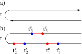
Real-time quantum dynamics can be generally represented as evolution along the so-called Keldysh contour $\mathcal{K}$, plotted in Fig. 1, made of two branches winding around the real-time axis from $0$ to $t$ (lower branch) and back from $t$ to $0$ (upper branch). In this perspective the average value of any operator $\mathcal{O}$ can be written as

$$\langle\mathcal{O}\left(t\right)\rangle=Tr\left\{\rho_{0}\>T_{\mathcal{K}}\left(e^{-i\int_{\mathcal{K}}\,d\tau\,\mathcal{H}\left(\tau\right)}\mathcal{O}\right)\right\},$$ (2)

where the trace is over the lead and impurity degrees of freedom and $T_{\mathcal{K}}$ denotes time-ordering along the Keldysh contour. The main idea of the approach is to expand the evolution operator (2) in powers of the hybridization and trace-out exactly the leads degrees of freedom. The expansion obtained in that way looks as the natural generalization of the diagrammatic expansion of Ref. Werner et al. (2006) to the $\mathcal{K}$ contour, which is required to deal with nonequilibrium effects. The resulting diagrams are then sampled with a Monte Carlo algorithm that we shall discuss in detail. To show how the method works, we start by considering a spinless biased resonant level model (RLM), namely a single fermionic energy level $\varepsilon_{d}$ driven out of equilibrium by an applied bias $eV=\mu_{L}-\mu_{R}$ between the two leads. Given an initial density matrix $\rho_{0}=\rho_{leads}\otimes\rho_{imp}$, with $\rho_{leads}$ describing the two uncoupled leads each at equilibrium with its own chemical potential and $\rho_{imp}=c^{\dagger}c$ – the impurity is initially occupied – we are interested in computing, for example, the real-time evolution of the RLM population $n=c^{{\dagger}}c$. To this extent, we expand the Keldysh evolution operator in powers of the hybrization between the bath and the impurity and trace out the lead degrees of freedom, which are non-interacting. The resulting expansion reads

$$\langle n(t)\rangle = \sum_{k=0}^{\infty}\sum_{n=0}^{k}(-1)^{k}\,\int_{0}^{t_{k}^{s}}dt_{k}^{e}\int_{0}^{t_{k-1}^{e}}dt_{k}^{s}\dots\int_{0}^{t_{k-n}^{s}}dt_{k-n}^{e}\int_{0}^{t}\,dt_{k-n}^{s}$$ (3)

$$\int_{0}^{t}dt_{k-n-1}^{e}\int_{0}^{t_{k-n-1}^{e}}dt_{k-n-1}^{s}\dots\int_{0}^{t_{2}^{s}}dt_{1}^{e}\int_{0}^{t_{1}^{e}}dt_{1}^{s}\,\mathcal{D}_{k}\left(t_{1}^{e},\dots,t_{k}^{e}|t_{1}^{s},\dots,t_{k}^{s}\right)\,\mathcal{L}_{k}\left(t_{1}^{e},\dots,t_{k}^{e}|t_{1}^{s},\dots,t_{k}^{s}\right)$$

Here $\mathcal{D}_{k}$ is the outcome of tracing the lead degrees of freedom and can be expressed in closed form as the determinant of a $k\times k$ matrix $\mathcal{M}^{-1}$,

$$\mathcal{D}\left(t_{1}^{e},\dots,t_{k}^{e}|t_{1}^{s},\dots,t_{k}^{s}\right)=det\,\left(\mathcal{M}^{-1}\right),$$ (4)

whose entries are the Keldysh hybridization functions

$$\mathcal{M}^{-1}_{ij}=i\Delta_{\mathcal{K}}\left(t_{i}^{e},t_{j}^{s}\right)\,s\left(t_{i}^{e},t_{j}^{s}\right),$$ (5)

which we define as

$$\Delta_{\mathcal{K}}\left(t^{e},t^{s}\right)=\sum_{k\alpha}|V_{k\alpha}|^{2}\langle T_{\mathcal{K}}\left(f^{\phantom{\dagger}}_{k\alpha}\left(t^{e}\right)f^{{\dagger}}_{k\alpha}\left(t^{s}\right)\right)\rangle\,.$$ (6)

Here we adopt the standard definition of the Keldysh Green’s functions Rammer (2008), namely we consider $t^{s},t^{e}$ as living on the contour $\mathcal{K}$. We note the additional sign $s\left(t^{e},t^{s}\right)$, which is negative when the two times are on opposite branches and positive otherwise. While the determinant $\mathcal{D}_{k}$ properly accounts for the effects associated to the leads, the function $\mathcal{L}_{k}$ involves only the impurity degrees of freedom and can be generally written as a trace over the initial impurity density matrix, namely

$$\mathcal{L}_{k}=Tr\bigg{\{}\rho_{imp}\,T_{\mathcal{K}}\left(c^{{\dagger}}(t^{e}_{k})c(t_{k}^{s})\dots c^{{\dagger}}(t^{e}_{1})c(t_{1}^{s})n(t)\right)\bigg{\}}.$$ (7)

The expansion thus obtained admits a natural representation in terms of a collection of $k$ segments, $t\in\left[t^{s}_{i},t^{e}_{i}\right]$, or equivalently $k-1$ anti-segments, $t\in\left[t^{e}_{i},t^{s}_{i+1}\right]$, properly ordered along the contour $\mathcal{K}$ and connected in all possible ways by the Keldysh hybridization functions $\Delta_{\mathcal{K}}(t^{e},t^{s})$. An example of such a configuration for $k=3$ is plotted in fig. 1. It is worth noticing that a similar expansion can be carried out also for other quantities like e.g. the average current $\langle I_{\alpha}(t)\rangle$ or the noise $S(t)=\langle I_{\alpha}(t)I_{\alpha}(0)\rangle$, resulting into a very general approach.
Algorithm. As usual in DiagMC Rubtsov et al. (2005); Werner et al. (2006) we view the perturbative expansion as a sum over configurations $\mathcal{C}$, i.e. diagrams with $k$ segments placed along the contour $\mathcal{K}$. In order to get an efficient sampling scheme three basic updates are implemented: adding/removing a segment, adding/removing an antisegment or shifting a segment end-point. We accept/reject a new configuration according to detailed balance prescription. In the actual simulation, we store and update the matrix $\mathcal{M}$ defined in (5), which is the only quantity required to compute Metropolis acceptance ratios Rubtsov et al. (2005).
Benchmark. We benchmark the method in the biased spinless RLM, which can be exactly solved hence being the simplest test for a real-time diagMC calculation. In fact, the main issue when sampling real-time quantum dynamics is the so called sign-problem, namely the exponential increase of relative errors in the Monte Carlo estimate of any observable in the infinite-size (or zero temperature) limit. This is well known in thermal-equilibrium (imaginary-time) Monte Carlo simulations of fermionic systems. In this perspective, diagrammatic Monte Carlo has been proved to be a generic sign-tolerant approach which can deal with sign-alterning series and even take advantage from them Prokof’ev and Svistunov (2007). How far this approach can be pushed, in particular in studying real-time dynamics, is the main scope of this work. To this extent, we compute the occupation number $\langle n(t)\rangle$ as a function of time $t$ for different values of the level position $\varepsilon_{d}$ both in equilibrium, $eV=0$, as well as out of equilibrium, $eV\neq 0$, and compare the exact results with diagMC data. 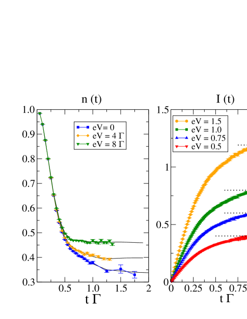In this simple case, we expect that a single energy scale, namely the level broadening $\Gamma=\pi\sum_{k}\,|V_{k}|^{2}\delta(\varepsilon_{k})$, controls the approach to the steady-state. As can be seen from Fig. 2, this is indeed confirmed by diagMC calculation which perfectly matches the exact solution. Indeed, we are able to resolve both the short-time decay from the initial configuration as well as the approach to the steady state. We note that a finite applied bias, $eV\neq 0$, cuts off the Keldysh evolution operator (2) (the steady state is reached earlier than at $eV=0$), as pointed out by Ref. Mitra et al. (2005), thus making the expansion more convergent. As mentioned previously, within the present approach one can easily measure the current flowing thorugh the impurity $I(t)=\frac{1}{2}\langle I_{L}(t)-I_{R}(t)\rangle$ on a fine real-time grid in a very efficient way, which is also shown in Fig. 2. It is worth mentioning that within our Keldysh diagMC we are able to reach a true non-equilibrium steady state with a finite value of the current, due to the infinite size of the bath. Dissipation occurs entirely within the fermionic reservoir and we do not need to include any ficticious bosonic bath to reach a steady state.

Figure 2: Zero-temperature real-time dynamics for different bias values $eV$ of the dot population, $\langle n(t)\rangle$, from an initially occupied dot (left panel) and of the current, $\langle I(t)\rangle$ (right panel) of the resonant level model. DiagMC results (dots) are compared with the exact solution (full line). We take $\epsilon_{d}=\Gamma$ and consider a flat density of states in the leads with an half-bandwidth $10\Gamma$.

Nonequilibrium Transport through a single-molecule. As a first non trivial application we consider a simple model of a molecular conductor, namely a spinless fermionic level coupled to Holstein phonon. The local Hamiltonian reads

$$\mathcal{H}_{loc}(n)=\frac{\omega_{0}}{2}(x^{2}+p^{2})+gx(n-\frac{1}{2})+\varepsilon_{d}(n-\frac{1}{2})$$ (8)

where $\omega_{0}$ is the phonon frequency (with displacement $x$ and its conjugate variable $p$), $\varepsilon_{d}$ is the energy of the level and $n$ its occupancy and finally $g$ the electron-phonon coupling. Our Keldysh diagMC can be naturally extendend to include local phonons, the only difference appears in the trace over local degrees of freedom (7), which now involves fermionic operators evolved according to the hamiltonian (8) for the electron-phonon subsystem. This trace can be evaluated analytically by observing that the local Hamiltonians with different level occupancy $n=0,1$ are related one to the other by a unitary transformation, $\mathcal{H}_{loc}(0)+\epsilon_{d}=U^{{\dagger}}\mathcal{H}_{loc}(1)U$, with $U=\exp\left(igp/\omega_{0}\right)$. It follows that the bosonic contribution to the local trace reduces to the following bosonic correlation-function

$$\mathcal{L}^{ph}_{k}=Tr\Bigg{(}\rho_{ph}\,U^{\dagger}(t^{e}_{k})\,U(t^{s}_{k})\,U^{\dagger}(t^{e}_{k-1})\dots U(t^{s}_{1})\Bigg{)},$$ (9)

which can be easily evaluated analytically for most common initial phonon density matrices $\rho_{ph}$, which we assume the equlibrium distribution at zero temperature. In (9) $U(t)$ and $U^{\dagger}(t)$ are the unitary operators evolved with $\mathcal{H}_{loc}(1)$, and we have assumed the level initially occupied. Therefore local vibrational degrees of freedom can be included in our sampling scheme at any order in the coupling constant $g$, allowing to extract by Keldysh DiagMC non-perturbative results in the electron-phonon coupling.

Figure 3: Zero-temperature differential conductance $dI/dV$ (in unit of $e^{2}/h$) for bias values $eV$ around $\omega_{0}=2.0\Gamma$. Electron-phonon coupling is $g=0.5\omega_{0}$. We consider two different values of the fermionic level position $\varepsilon_{d}$ in order to reproduce the crossover from reducted (step-down) to enhanced (step-up) conductance.

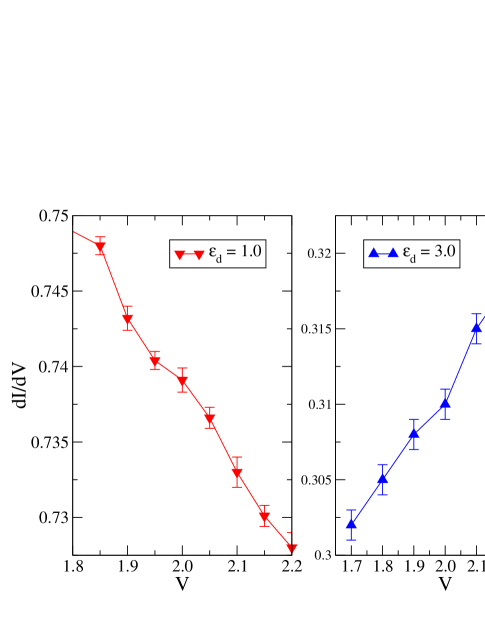
The coupling to molecular vibrations is known to significantly affect inelastic electron tunneling. Galperin et al. (2007) When the bias hits a vibrational frequency, the differential conductance $dI/dV$ changes sharply. Experimentally it is observed that $dI/dV$ increases in the tunneling regime, but decreases in the opposite case of a high transmission barrier. Although simple physical arguments can be invoked Jaklevic and Lambe (1966); Persson (1988); Agraït et al. (2002) to explain this phenomenon, theoretical calculations within the Keldysh formalism have so bar been restricted to the lowest orders in the electron-phonon coupling. de la Vega et al. (2006); Paulsson et al. (2008); Egger and Gogolin (2008) In the simple resonant level model that we are considering, the perturbative calculations predict that $dI/dV$, at bias $eV=\omega_{0}$, should decrease if the zero-bias conductance $G>0.5$, in units of the unitary value (in our spinless case $e^{2}/h$), otherwise should increase. de la Vega et al. (2006); Paulsson et al. (2008); Egger and Gogolin (2008) Evidences in favor of this results have been very recently found by Tal and coworkers with H₂O molecules bridging a Pt break-junction. Since the Keldysh diagMC is, as mentioned, non perturbative in the electron-phonon coupling, it offers the possibility to verify the above theoretical predictions. We model the two regimes of $G\gtrless 0.5$ by two different values of the level position $\varepsilon_{d}=1$ and 3, the former closer to resonance than the latter, and compute directly the differential conductance $dI/dV$. As can be seen from Fig. 3 a step-down or step-up features do appear around the threshold for vibronic excitations, $eV\simeq\omega_{0}$, when the zero bias conductance is greater or lower than $0.5$, respectively, in agreement with perturbative results. de la Vega et al. (2006); Paulsson et al. (2008); Egger and Gogolin (2008) We also note that the step is not as abrupt as found in perturbation theory de la Vega et al. (2006); Paulsson et al. (2008); Egger and Gogolin (2008), likely signaling a significant phonon damping.

In summary, we have introduced a novel non perturbative approach to nonequilibrium quantum transport in nanoscopic conductors. The method is based on a Diagrammatic Monte Carlo sampling of the real-time perturbation theory in the impurity-leads hybridization, performed along the Keldysh contour required to treat non equilibrium effects. In spite of the oscillating nature of the real-time quantum evolution, we are able to follow the dynamics starting from an arbitrary initial preparation up to the steady state. This is primarily due to the combined effects of infinite leads and of the applied bias, which cut-off the Keldysh evolution operator, but also to the capability of the algorithm to cope with sign-problem. As a first application we have studied zero temperature non linear transport through a simple model of a molecular conductor. Being a completely general method, it can be in principle used to study any discrete quantum system bridging two non-interacting conducting leads, providing a new tool to study quantum transport in nanoscopic devices.

References

- Tao (2006) N. J. Tao, Nature Nanotechnology 1, 173-181 (2006).
- Cuniberti et al. (2005) G. Cuniberti, G. Fagas, and K. Richter, Introducing Molecular Electronic (Springer Berlin and Heidelberg, 2005).
- Goldhaber-Gordon et al. (1998) D. Goldhaber-Gordon, J. Göres, M. A. Kastner, H. Shtrikman, D. Mahalu, and U. Meirav, Phys. Rev. Lett. 81, 5225 (1998).
- Park et al. (2000) H. Park, J. Park, A. Lim, E. Anderson, A. ALivisatos, and P. Mcuen, Nature 407, 57 (2000).
- Parks et al. (2007) J. J. Parks, A. R. Champagne, G. R. Hutchison, S. Flores-Torres, H. D. Abruna, and D. C. Ralph, Phys. Rev. Lett. 99, 026601 (2007).
- Stinaff et al. (2006) E. A. Stinaff, M. Scheibner, A. S. Bracker, I. V. Ponomarev, V. L. Korenev, M. E. Ware, M. F. Doty, T. L. Reinecke, and D. Gammon, Science 311, 636 (2006).
- Shi et al. (2007) S.-F. Shi, K. I. Bolotin, F. Kuemmeth, and D. C. Ralph, Phys. Rev. B 76, 184438 (2007).
- Tal et al. (2008) O. Tal, M. Krieger, B. Leerink, and J. M. van Ruitenbeek, Phys. Rev. Lett. 100, 196804 (2008).
- Bulla et al. (2008) R. Bulla, T. A. Costi, and T. Pruschke, Rev. Mod. Phys. 80, 395 (2008).
- Rubtsov et al. (2005) A. N. Rubtsov, V. V. Savkin, and A. I. Lichtenstein, Phys. Rev. B 72, 035122 (2005).
- Werner et al. (2006) P. Werner, A. Comanac, L. de’ Medici, M. Troyer, and A. J. Millis, Phys. Rev. Lett. 97, 076405 (2006).
- Governale et al. (2008) M. Governale, M. G. Pala, and J. König, Phys. Rev. B 77, 134513 (2008).
- Anders and Schiller (2005) F. B. Anders and A. Schiller, Phys. Rev. Lett. 95, 196801 (2005).
- Weiss et al. (2008) S. Weiss, J. Eckel, M. Thorwart, and R. Egger, Phys. Rev. B 77, 195316 (2008).
- Mühlbacher and Rabani (2008) L. Mühlbacher and E. Rabani, Phys. Rev. Lett. 100, 176403 (2008).
- Rammer (2008) J. Rammer, Quantum Field Theory of Nonequilibrium States (Cambridge University Press, 2008).
- Prokof’ev and Svistunov (2007) N. Prokof’ev and B. Svistunov, Phys. Rev. Lett. 99, 250201 (2007).
- Mitra et al. (2005) A. Mitra, I. Aleiner, and A. J. Millis, Phys. Rev. Lett. 94, 076404 (2005).
- Galperin et al. (2007) M. Galperin, M. Ratner, and A. Nitzan, J.Phys.: Condens. Matter 19, 103201 (2007).
- Jaklevic and Lambe (1966) R. C. Jaklevic and J. Lambe, Phys. Rev. Lett. 17, 1139 (1966).
- Persson (1988) B. Persson, Phys. Scr. 38, 282 (1988).
- Agraït et al. (2002) N. Agraït, C. Untiedt, G. Rubio-Bollinger, and S. Viera, Chem. Phys. 281, 231 (2002).
- de la Vega et al. (2006) L. de la Vega, A. Martin-Rodero, N. Agrait, and A. L. Yeyati, Phys. Rev.B 73, 075428 (2006).
- Paulsson et al. (2008) M. Paulsson, T. Frederiksen, H. Ueba, N. Lorente, and M. Brandbyge, Phys. Rev. Lett. 100, 226604 (2008).
- Egger and Gogolin (2008) R. Egger and A. Gogolin, Phys. Rev. B 77, 113405 (2008).