Application of Data Assimilation Method for Predicting Solar Cycles

Abstract

Despite the known general properties of the solar cycles, a reliable forecast of the 11-year sunspot number variations is still a problem. The difficulties are caused by the apparent chaotic behavior of the sunspot numbers from cycle to cycle and by the influence of various turbulent dynamo processes, which are far from understanding. For predicting the solar cycle properties we make an initial attempt to use the Ensemble Kalman Filter (EnKF), a data assimilation method, which takes into account uncertainties of a dynamo model and measurements, and allows to estimate future observational data. We present the results of forecasting of the solar cycles obtained by the EnKF method in application to a low-mode nonlinear dynamical system modeling the solar $\alpha\Omega$-dynamo process with variable magnetic helicity. Calculations of the predictions for the previous sunspot cycles show a reasonable agreement with the actual data. This forecast model predicts that the next sunspot cycle will be significantly weaker (by $\sim 30\%$) than the previous cycle, continuing the trend of low solar activity.

1 Introduction

Investigation of solar activity is one of the oldest solar physics problems. Here we consider this phenomenon in the context of the sunspot number variations, which have detailed observational data during the past 23 solar cycles. There is no doubt that the 11-year cyclic variations of the sunspot number are connected to the dynamo process inside the Sun. Therefore it is natural to search for a solution by investigating nonlinear dynamo models, and use them for predicting the solar cycles. However, our current understanding of the solar dynamo is quite poor. The current predictions of the next solar cycle, number 24, show a wide range of the expected sunspot number. For example, using an axisymmetric, mean-field model of a flux transport dynamo Dikpati and Gilman (2006) predicted that the cycle 24 will be about 30% - 50% stronger than the previous cycle 23 with the sunspot number reaching 155 - 180 at the maximum. Using polar magnetic field measurements and assuming a direct relationship between the polar field strength and the future toroidal magnetic field Svalgaard et al. (2005) predicted that the cycle 24 will have a peak sunspot number of $75\pm 8$. A weak cycle 24 with the sunspot number of $74\pm 10$ was also proposed by Javaraiah (2007) from analysis of sums of the areas of sunspot groups in the latitudinal interval of $0^{\circ}-10^{\circ}$ in both hemispheres. There are many other predictions for the upcoming cycle(s), reviewed by Kane (2007) and Obridko and Shelting (2008).

The great variety of the predictions is caused by uncertainties in the dynamo models and model parameters, and errors in both models and observations. In the paper, we present initial results of application of a data assimilation method to a simple nonlinear dynamo model (Kitiashvili & Kosovichev, 2008). This model reproduces the basic properties of a solar cycle, such as the shape of the sunspot number profile. The advantage of the data assimilation methods is in their ability to combine the observational data and the models for possible efficient and accurate estimations of the physical properties, which cannot be observed directly. Here we consider an implementation of the Ensemble Kalman Filter method, EnKF, (Evensen, 2007), which is effective for investigation of nonlinear dynamical models. The method is useful in several aspects: it supports estimations of past, present, and even future states of a system, and it can do so even when the precise nature of a modeled system is unknown.

2 Basic formulation of the data assimilation method

The main goal of any model is an accurate description of properties of a system in the past and present times, and the prediction of its future behavior. However, a model is usually constructed with some approximations and assumptions, and has errors. Therefore, it cannot describe the true condition of a system. On the other hand, observational data, $d$, also include errors, $\epsilon$, which are often difficult to estimate. The data assimilation methods such as the Kalman Filter (Kalman, 1960) allow us, with the help of an already constructed model and observational data, to determine the initial state of the model, which will be in agreement with a set of observations, and obtain a forecast of future observations and estimate its errors (Evensen, 2007; Kitiashvili, 2008). For instance, in our case we know from observations the sunspot number (with some errors) and want to estimate the state of the solar magnetic fields, described by a dynamo model.

In generally, if the state, $\psi$, of a system can be described by a dynamical model $d\psi/dt=g(\psi,t)+q$, with initial conditions $\psi_{0}=\Psi_{0}+p$, where $g(\psi,t)$ is a nonlinear vector-function, $q$ and $p$ are the errors of the model and in the initial conditions, then the system forecast is $\psi^{f}=\psi^{t}+\phi$, where $\psi^{t}$ is the true system state, and $\phi$ is the forecast error. The relationship between the true state and the observational data is given by a relation $d=M[\psi]+\epsilon$, where $d$ is a vector of measurements, $M[\psi]$ is a measurement functional, which relates the model state, $\psi$, to the observations, $d$.

For a realization of the data assimilation procedure in the case of nonlinear dynamics it is convenient to use the Ensemble Kalman Filter (EnKF) method (Evensen, 2007). The main difference of the EnKF from the standard Kalman Filter is in using for the analysis an ensemble of possible states of a system, which can be generated by Monte Carlo simulations. If we have an ensemble of measurements $d_{j}=d+\epsilon_{j}$ with errors $\epsilon_{j}$ (where $j=1,...,N$) then we can define the covariance matrix of the measurement errors $C_{\epsilon\epsilon}^{e}=\overline{\epsilon\epsilon^{T}}$, where the over bar means the ensemble averaged value, and superscript $T$ indicates transposition. Using a model we always can describe future states of a system, $\psi^{f}$. However, errors in the model, initial conditions and measurements do not allow the model result be consistent with observations. To take into account this deviation, we consider a covariance matrix of the first guess estimates (our forecast related only to model calculations): $(C_{\psi\psi}^{e})^{f}=\overline{(\psi^{f}-\overline{\psi^{f}})(\psi^{f}-\overline{\psi^{f}})^{T}}$. Note, that the covariance error matrix is calculated for every ensemble element. Then, the estimate of the system state is given by:

$$\psi^{a}=\psi^{f}+K\left(d-M\psi^{f}\right),$$ (1)

where $K=(C_{\psi\psi}^{e})^{f}M^{T}\left(M(C_{\psi\psi}^{e})^{f}M^{T}+C_{\epsilon\epsilon}^{e}\right)^{-1}$, is the so-called Kalman gain (Kalman, 1960; Evensen, 2007). The covariance error matrix of the best estimate is calculated as: $(C_{\psi\psi}^{e})^{a}=\overline{(\psi^{a}-\overline{\psi^{a}})(\psi^{a}-\overline{\psi^{a}})^{T}}=\left(I-K_{e}M\right)(C_{\psi\psi}^{e})^{f}$. We can use the last best estimate obtained with the available observational data as the initial conditions and make the next forecast step. At the forecast step, we calculate a reference solution of the model, according to the new initial conditions, then simulate measurements by adding errors to the model and to the initial conditions. Finally we obtain a new best estimate of the system state, which is our forecast. A new set of observations allows us to redefine the previous model state and make a correction to the predicted state.

In order to implement EnKF for prediction of the sunspot cycles it is necessary to define a dynamo model, which describes the evolution of the system parameters in time.

3 Dynamo model

Currently, there is no generally accepted model of the solar dynamo. However, most of the models are based on the Parker’s oscillatory $\alpha\Omega$-dynamo mechanism (Parker, 1955), which includes turbulent helicity and magnetic field stretching by the differential rotation. Recent observational and theoretical investigations (e.g. Sokoloff, 2007; Brandenburg & Subramanian, 2005) revealed an important role of magnetic helicity (Pouquet et al., 1976). Thus, for this investigation we added to the original Parker’s model an equation describing the evolution of the magnetic helicity, $\alpha_{m}$. This equation was derived by Kleeorin and Ruzmaikin (1982) from the conservation of the total magnetic helicity. Then, the dynamo model can be written as (Kitiashvili & Kosovichev, 2008)

$$\frac{\partial A}{\partial t} = \alpha B+\eta\nabla^{2}A,\,\,\frac{\partial B}{\partial t}=G\frac{\partial A}{\partial x}+\eta\nabla^{2}B,$$ (2)

$$\frac{\partial\alpha_{m}}{\partial t} = \frac{Q}{2\pi\rho}\left[\langle{\vec{B}}\rangle(\nabla\times\langle{\vec{B}}\rangle)-\frac{\alpha}{\eta}\langle{\vec{B}}\rangle^{2}\right]-\frac{\alpha_{m}}{T},$$

where $B$ is the toroidal component of magnetic field, $A$ is the vector potential of the poloidal component of the mean magnetic field, $\langle\vec{B}\rangle=\vec{B}_{P}+\vec{B}_{T}$ ($\vec{B}_{P}={\rm curl}(0,0,A)$, $\vec{B}_{T}=(0,0,B)$ in spherical coordinates), $\eta$ describes the total magnetic diffusivity, which is the sum of the turbulent and molecular magnetic diffusivity, $\eta=\eta_{t}+\eta_{m}$ (usually $\eta_{m}<<\eta_{t}$); $G=\partial\left<v_{x}\right>/\partial y$ is the rotational shear, coordinates $x$ and $y$ are in the azimuthal and latitudinal directions respectively, parameter $\alpha$ is helicity represented in the form $\alpha=\alpha_{h}/(1+\xi B^{2})+\alpha_{m}$, $\alpha_{h}$ and $\alpha_{m}$ are the kinetic and magnetic parts; $\xi$ is a quenching parameter, $\rho$ is density, $T$ is a characteristic time of dissipation magnetic helicity (which includes dissipation though helicity transport) and, $Q\sim 0.1$.

Following the approach of Weiss et al. (1984) we average the system of equations (2) in a vertical layer to eliminate $z$-dependence of $A$ and $B$ and consider a single Fourier mode propagating in the $x$-direction assuming $A=A(t)e^{ikx}$, $B=B(t)e^{ikx}$; then we get the following system of equations

$$\frac{{\rm d}A}{{\rm d}t} = \alpha B-\eta k^{2}A,\qquad\frac{{\rm d}B}{{\rm d}t}=ikGA-\eta k^{2}B,$$ (3)

$$\frac{{\rm d}\alpha_{m}}{{\rm d}t} = -\frac{\alpha_{m}}{T}-\frac{Q}{2\pi\rho}\left[-ABk^{2}+\frac{\alpha}{\eta}\left(B^{2}-k^{2}A^{2}\right)\right].$$

For the interpretation of the solutions of the dynamical system in terms of the sunspot number properties we use the imaginary part of the toroidal component $B(t)$ because it gives the amplitude of the antisymmetric harmonics, and approximate the sunspot number, $W$, as $({\rm Im}B)^{3/2}$, following Bracewell’s suggestion (Bracewell, 1953, 1988). This dynamo model has been investigated in detail by Kitiashvili & Kosovichev (2008).

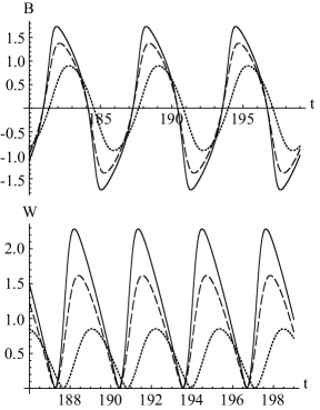
Figure 1 shows typical nonlinear periodic solutions and the corresponding model sunspot number, which reproduce typical observed solar cycle profiles with fast growth and slow decay. The profile of the toroidal field variations becomes close to the sinusoidal behavior for small amplitude. Perhaps, it is essential that the model gives a qualitatively correct relationship between the model sunspot number amplitude and the growth time.

4 Implementation of Ensemble Kalman Filter

For the assimilation of the sunspot data into the dynamo model we selected a class of periodic solutions, which corresponds to parameters of the middle convective zone and describes the typical behavior of the sunspot number variations (Fig. 1). The implementation of the EnKF method consists of 3 steps: preparation of the observational data for analysis, correction of the model solution according to observations, and prediction.

Step 1: Preparation of the observational data. Following Bracewell (1953, 1988), we transform the annual smoothed values of the sunspot number for the period of 1856 - 2007 in the toroidal field values using the relationship $B\sim W^{2/3}$ and alternating the sign of $B$. Also we select the initial conditions of the model so that the reference solution coincides with the beginning of the first cycle of our series, cycle 10, which started in 1856. In this paper we do not consider the previous solar cycles because of the uncertainties in the early sunspot number measurements (Svalgaard et al., 2007). Then we normalize the toroidal field in the model in such a way that the model amplitude of $B$ is equal to the mean ”observed” toroidal field. In addition, we normalize the model time scale assuming that the period of the model sunspot variations corresponds to the typical solar cycle duration of 11 years.

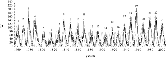
Step 2: Assimilation for the past system state. Unfortunately we do not have observations of the magnetic helicity, toroidal and poloidal components of magnetic field. Therefore, in the first approximation, we generate observational data as random values around the reference solution with a standard deviation of $\sim 12\%$, which was chosen to roughly reproduce the observed variations of the sunspot number. Similar random errors are also added to the model equations as described in Sec. 2. Then, we calculate the covariance error matrixes of the observations, $C_{\epsilon\epsilon}^{e}$, and the forecast, $(C_{\psi\psi}^{e})^{f}$. After combining the observational and model error covariances in the form of Kalman gain, $K$, we obtain the best estimate of evolution of the system, $\psi^{a}$ from Eq. 1. Figure 2 shows the result of assimilation of the sunspot data into the dynamo model: the best EnKF estimate (black curve), the initial model (grey curve) and the actual sunspot data (circles).

Step 3: Prediction. For obtaining a prediction of the next solar cycle we determine the initial conditions from the best estimated solution for the previous cycle in terms of the amplitude and phase to continue the model calculations. Then after receiving the reference solution with the new initial conditions we simulate future observational data by adding random noise and repeat the analysis. This provides the best EnKF estimate of the future state of the system (forecast).

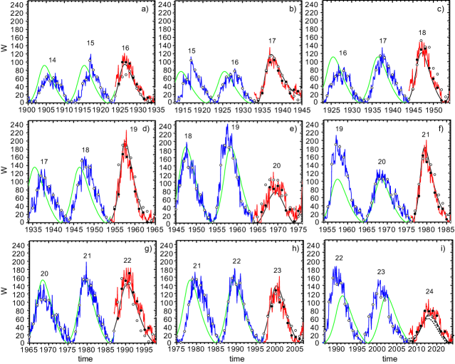
The described analysis has been tested by calculating predictions of the previous cycles. Figure 3 (a-h) shows the examples of the EnKF method implementation for forecasting the sunspot number of cycles 16-23. For these forecasts, we first obtain the best estimated solutions (blue curves) using the observational data prior to these cycles (open circles). After this, we obtain the exact solution (black curves) according to the initial conditions of the time of the last measurement and simulate a new set observation (black dots) by adding random noise. Then, we obtain the EnKF estimates using the simulated observations, which give us the prediction (Fig. 3, red curves). These experiments show that this approach can provide reasonable forecast of the strength of the next solar cycles. However, there are significant discrepancies. For instance, the strength of the cycle 16 is overestimated, and the strength of cycle 19 is underestimated. The main uncertainties are caused by in accuracies in determining the time of the end of the previous cycle from the sunspot number data, and, of course, by the incompleteness of the model and insufficiency the sunspot number data. In particular, we found the forecast is inaccurate when the sunspot number change significantly from the value of the previous cycle. Also, our forecast experiments showed a strong dependence on the phase relation between the reference model solution and the observations. The phase difference appears due to the constant period of the solution the variations in the duration of the solar cycles. Curiously, when the model phase is ahead of the solar cycle phase then adding a data point at the start of a cycle substantially improves the forecast. However, when the model phase lags thai does not happen. This effect is taken into account by correcting the phase of the reference solution that it is slightly ahead of the solar cycle phase.

The same analysis scheme is applied for prediction of the next solar cycle 24 (Fig. 3i). According to this result, the solar cycle 24 will be weaker than the current cycle by approximately 30%. To check the stability of the prediction we used two other sets of initial conditions in 2008 and obtained close results (Fig. 3i).

5 Discussion and Conclusion

The results of assimilation of the annual sunspot number data into the solar dynamo model and the prediction of the previous solar cycles (Fig. 3) demonstrate a new method of forecasting the solar activity cycles. Using the EnKF method and a simple dynamo model we obtained reasonable predictions usually for the first halfs of the sunspot cycles with the error $\sim 8-12$%, and in some cases also for the declining phase of the cycles. This method predicts a weak solar cycle 24 (Fig. 3i) with the smoothed annual sunspot number at the maximum of approximately 80. It is interesting that the simulations show that the previous cycle does not finish in 2007 as was expected, but it still continues. According to the estimates the maximum of the next cycle will be approximately in 2013.

The application of the data assimilation method, EnKF, for modeling and predicting the solar cycles shows the power of this approach and encourages further development. It also reveals significant uncertainties in the model and the data. Among these are the uncertainties in the determination of the start of a solar cycle from the sunspot number series (in particular, when the cycles overlap), leading to the uncertainty in the phase relation between the model solution and the data. Also, there are significant uncertainties in the relationship between the sunspot number data and the physical properties of the solar magnetic field, in the absence of magnetic field and helicity data, and, of course, in the dynamo model. Our conclusion is that for robust and accurate predictions of the solar cycles the information contained in the sunspot number data is insufficient. For further development we plan to apply the data assimilation method to more complete 2D dynamo models, which describe the latitudinal distribution of the solar magnetic field, and use the magnetograph data available for the past 3 cycles.

This work was supported by the Center for Turbulence Research (Stanford) and the International Space Science Institute (Bern).

Figure 1: A typical periodic solution (in non-dimensional units) of the dynamo model: toroidal magnetic field, $B$ (top panel), and the model sunspot number, $W$ (bottom panel) (Kitiashvili & Kosovichev, 2008).

Figure 2: Results of assimilation of the annual sunspot number data (circles) into the dynamo model. The grey curve shows the reference solution (without assimilation analysis), and the black curve shows the best EnKF estimate of the sunspot number variations, obtained from the data and the dynamo model.

Figure 3: Predictions for the solar cycles 16-24. The green curves show the model reference solution. The blue curves show the best estimate of the sunspot number using the observational data (empty circles) and the model, for the previous cycles. The black curve the model solution according to the initial conditions of the last measurement. The red curves show the prediction results. In panel i) the model solution is shown for 3 different estimates of the sunspot number for 2008: 3 (black curve), 5 (dashes) and 10 (dots).

References

- Bracewell (1953) Bracewell, R.N. 1953, Nature, 171, 649.
- Bracewell (1988) Bracewell, R.N. 1988, MNRAS, 230, 535.
- Brandenburg & Subramanian (2005) Brandenburg, A. & Subramanian, K. 2005, Physics Reports, 417, 1.
- Dikpati & Gilman (2006) Dikpati, M. & Gilman, P.A. 2006, ApJ, 649, 498.
- Evensen (2007) Evensen, G. Data assimilation. Springer. 2007.
- Javaraiah (2007) Javaraiah, J. 2007, MNRAS, 377, L34.
- Kalman (1960) Kalman, R.E. 1960, J. Basic. Eng., 82, 35.
- Kane (2007) Kane, R.P. 2007, Solar Physics, 246, 471.
- Kitiashvili (2008) Kitiashvili, I. 2008, ASP Conf. Series, 383, 255.
- Kitiashvili & Kosovichev (2008) Kitiashvili, I.N. & Kosovichev, A.G. 2008, Geophys. Astrophys. Fluid Dyn. in press.
- Kleeorin & Ruzmaikin (1982) Kleeorin, N.I. & Ruzmaikin, A.A. 1982, Magnetohydrodynamics, 18, 116.
- Obridko & Shelting (2008) Obridko, V.N. & Shelting, B.D. 2008, Solar Physics, 248, 191.
- Parker (1955) Parker, E.N. 1955, ApJ, 122, 293.
- Pouquet et al. (1976) Pouquet, A., Frisch, U. & Léorat, J. 1976, J. Fluid Mech., 77, 321.
- Sokoloff (2007) Sokoloff, D. 2007, Plasma Phys. Control. Fusion, 49, B447.
- Svalgaard et al. (2005) Svalgaard, L., Cliver, E.W. & Kamide Y. 2005, Geophys. Res. Lett., 32, L01104.
- Svalgaard et al. (2007) Svalgaard, L., Cliver, E.W. 2007, EOS Trans. AGU, 88(23), Abs.SH54B-02.
- Weiss et al. (1984) Weiss, N.O., Cattaneo, F. & Jones C.A. 1984, Geophys. Astrophys. Fluid Dyn., 30, 305.